SPA 3e_ Teachers Edition _ Ch 6

More documents

Recommendations

Info

dd dd d d dddddd 412 C H A P T E R 6 • Sampling Distributions Teaching Tip Have students look closely at the bottom dotplot in Figure 6.4 and the dotplot in the next example. Ask them if this simulated sampling distribution has a familiar shape. Later in this chapter, students will learn that certain statistics have approximately normal sampling distributions. Alternate Example Can you hand me that wrench? Sampling variability PROBLEM: A local auto parts store has records of the daily sales of hand tools (in dollars) over the last several years. To estimate the average daily sales, a manager selects 10 days and finds the sample mean daily sales. Here is a simulated sampling distribution of x, the sample mean daily sales of hand tools (in dollars) for 1000 samples of size n 5 10. a FigUre 6.4 Simulated sampling distributions of the sample proportion p^ for samples of size n 5 10 and samples of size n 5 50 from a population with p 5 0.7. e XAMPLe n = 10 n = 50 d d d d d d d d d d ddddddddddddddddddd 0.2 0.3 0.4 0.5 0.6 0.7 0.8 0.9 1.0 Sample proportion who take the bus As expected, both simulated sampling distributions have means near p 5 0.70. Also, the sampling distribution of p^ is much more variable when the sample size is n 5 10, compared with n 5 50. In a small sample, it is plausible that the sample proportion could be much smaller or much larger than the parameter, just by chance. However, when the sample size gets bigger, we expect the sample proportion to be fairly close to the value of the parameter. The lifetime of batteries: Hours or days? Sampling variability Decreasing sampling variability The sampling distribution of any statistic will have less variability when the sample size is larger. PROBLEM: For quality control, workers at a battery factory regularly select random samples of batteries to estimate the mean lifetime. Here is a simulated sampling distribution of x, the sample mean lifetime (in hours) for 1000 random samples of size n 5 100 from a population of AAA batteries. (a) What would happen to the sampling distribution of the sample mean x if the sample size were n 5 50 instead? Justify. (b) What is the practical consequence of this change in sample size? d d d dddd d d ddd dd dd d ddddddd d ddd ddd dd d ddd d d d ddd ddd dd d d dd ddd dd dd d dd dd ddd ddd d d d dd d dd d dd d dd dd d dd d dd d d d dd dddd dd d dd d dddd dd d dd d ddd d d d d dd d ddd ddd d dddd dd ddd dddd d d d d d d d ddd d ddd d d d d dd dd ddd d dd ddd ddd d dd d dd d dd dd d d dd d dddd ddd dd dddddddddd ddddddddd d ddd ddd d dddd dddd d ddd dddd d dddd ddd ddd ddd ddd d dddd d d d dddd d dd dd d dddd d ddd ddd d ddd dddd dddd dddd ddd d ddd ddd dddd ddd dd dd d d d d ddd dddd dddddd ddd dddd d dd d ddd ddd d dddd d dddd ddd d ddd d d dddd dd dd ddd d dd ddd d d dd dd d d d ddd d d ddddd ddddd ddd d ddd d ddd ddd ddd ddd ddd dddd dd ddd ddd ddd dd dd ddd dddddd dddd dd dd ddd d d dd d dd dd d ddd ddd dd d dddddd d dd d ddddd d ddd dd dd dd ddd d ddd d dd d dd d ddd ddd d d ddd d ddd d d d ddd ddd ddd ddd d d dddddd ddd ddd ddd ddd ddd d d dd d ddd d dd dd dddd d d ddd d ddd ddd dd d d d d dd d d d d d d d d d dd ddd ddd d d d d dd dd 100 120 140 160 180 200 220 Sample mean daily sales of hand tools ($) (a) What would happen to the sampling distribution of the sample mean x if the sample size were n 5 30 instead? Justify your answer. (b) What is the practical consequence of this change in sample size? SOLUTION: (a) The sampling distribution of the sample mean x will be less variable because the sample size is larger. (b) The estimated mean daily sales of hand tools will typically be closer to the true mean daily sales of hand tools. In other words, the estimate will be more precise. d SOLUTION: (a) The sampling distribution of the sample mean x will be more variable because the sample size is smaller. 44 46 48 50 52 54 56 58 60 62 Sample mean lifetime (h) (b) The estimated mean lifetime will typically be farther away from the true mean lifetime. In other words, the estimate will be less precise. FOR PRACTICE TRY EXERCISE 5. Starnes_3e_CH06_398-449_Final.indd 412 Putting It All Together: Center and Variability We can think of the true value of the population parameter as the bullseye on a target and of the sample statistic as an arrow fired at the target. Both bias and variability describe what happens when we take many shots at the target. • Bias means that our aim is off and we consistently miss the bullseye in the same direction. That is, our sample values do not center on the population value. 18/08/16 5:00 PMStarnes_3e_CH0 412 C H A P T E R 6 • Sampling Distributions Starnes_3e_ATE_CH06_398-449_v3.indd 412 11/01/17 3:54 PM
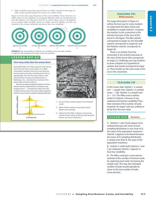
L E S S O N 6.2 • Sampling Distributions: Center and Variability 413 • High variability means that repeated shots are widely scattered on the target. In other words, repeated samples do not give very similar results. Figure 6.5 shows this target illustration of bias and variability. Notice that low variability (shots are close together) can accompany high bias (shots are consistently away from the bullseye in one direction). And low or no bias (shots center on the bullseye) can accompany high variability (shots are widely scattered). Ideally, we’d like our estimates to be accurate (unbiased) and precise (have low variability). d ddd dd dd High bias, low variability (a) d d d d d Low bias, high variability (b) d d d d d d High bias, high variability (c) d d d d d d d d d d d d FigUre 6.5 Bias and variability. (a) High bias, low variability. (b) Low bias, high variability. (c) High bias, high variability. (d) The ideal: no bias, low variability. L e SSon APP 6. 2 How many tanks does the enemy have? During World War II, the Allies captured many german tanks. Each tank had a serial number on it. Allied commanders wanted to know how many tanks the germans had so that they could allocate their forces appropriately. They sent the serial numbers of the captured tanks to a group of mathematicians in Washington, D.C., and asked for an estimate of the total number of german tanks N. Here are simulated sampling distributions for three statistics that the mathematicians considered, using samples of size n 5 7. The blue line marks N, the total number of german tanks. The shorter red line segments mark the mean of each simulated sampling distribution. Statistic 3 Statistic 2 Statistic 1 d d d d d d dd d d dd d d ddd dd ddd d dd dd d d d d ddd d d d d d dd d ddd dd d dddddd d ddd d d dd d d ddd ddd d d d d N Estimated total dd d ddd The ideal: no bias, low variability (d) 1. Do any of these statistics appear to be unbiased? Justify. 2. Which of these statistics do you think is best? Explain your reasoning. 3. Explain how the Allies could get a more precise estimate of the number of german tanks using the statistic you chose in Question 2. © Bettmann/Corbis Teaching Tip: Differentiate The target illustration in Figure 6.5 will be the best way for some students to understand the ideas of bias and variability in sample statistics. Compare the statistics in the screenshot in the Activity Overview at the start of this lesson to the figure. The Max statistic corresponds to target (a), the TwiceIQR statistic corresponds to target (b), and the Partition statistic corresponds to target (d). There is no statistic from the screenshot in the Activity Overview at the start of this lesson that corresponds to target (c). Challenge your top students to draw a dotplot of a hypothetical statistic that would correspond to target (c). They should use the same scale as the one in the screenshot. Teaching Tip In the Lesson App, Statistic 1 is sample min 1 sample max, Statistic 2 is sample mean 1 3SD, Statistic 3 is sample max· (n 1 1)/n. The Allies used a statistic similar to Statistic 3 because it was unbiased and had low variability! Thus, their estimate of the number of tanks would be “on target” and was unlikely to be far from the true value. Lesson App Answers Lesson 6.2 18/08/16 5:00 PMStarnes_3e_CH06_398-449_Final.indd 413 18/08/16 5:00 PM 1. Statistics 1 and 3 both appear to be unbiased because the mean of each sampling distribution is very close to N, the value of the population maximum. Statistic 2 appears to be biased because the mean of its sampling distribution is clearly more than N, the value of the population maximum. 2. Statistic 3; while both Statistics 1 and 3 are unbiased, Statistic 3 appears to have less variability. 3. The Allies could get a more precise estimate of the number of German tanks by capturing more tanks (increasing the sample size). This way, the estimated number of tanks would typically be closer to the true number of tanks (more precise). L E S S O N 6.2 • Sampling Distributions: Center and Variability 413 Starnes_3e_ATE_CH06_398-449_v3.indd 413 11/01/17 3:54 PM
Page 2 and 3: 6 Sampling Distributions Please rea
Page 4 and 5: Promoting Good Habits and Skills Ch
Page 6 and 7: Chapter 6 Resources SPA Applets hig
Page 8 and 9: PD Chapter 6 Overview Watch the cha
Page 10 and 11: PD LESSONS 6.1-6.3 Overview Watch t
Page 12 and 13: 402 C H A P T E R 6 • Sampling Di
Page 34 and 35: Answers continued 16. No; assuming
Page 42 and 43: Answers continued X 18. (c) p^ = n
Page 50 and 51: Activity answers continued 3. Yes,
Page 54 and 55: 9. (a) Because n = 50 ≥ 30, the s

SPA 3e_ Teachers Edition _ Ch 6

Create successful ePaper yourself

Delete template?

Save as template?