5128_Ch07_pp378-433

More documents

Recommendations

Info

Section 7.5 Applications from Science and Statistics 423 EXAMPLE 5 Probability of the Clock Stopping Find the probability that the clock stopped between 2:00 and 5:00. SOLUTION The pdf of the clock is 112, 0 t 12 f t { 0, otherwise. The probability that the clock stopped at some time t with 2 t 5 is 5 f t dt 1 4 . 2 Now try Exercise 27. ∫f(x)dx = .17287148 Figure 7.47 A normal probability density function. The probability associated with the interval a, b is the area under the curve, as shown. a b By far the most useful kind of pdf is the normal kind. (“Normal” here is a technical term, referring to a curve with the shape in Figure 7.47.) The normal curve, often called the “bell curve,” is one of the most significant curves in applied mathematics because it enables us to describe entire populations based on the statistical measurements taken from a reasonably-sized sample. The measurements needed are the mean m and the standard deviation s, which your calculators will approximate for you from the data. The symbols on the calculator will probably be Jx and s (see your Owner’s Manual), but go ahead and use them as m and s, respectively. Once you have the numbers, you can find the curve by using the following remarkable formula discovered by Karl Friedrich Gauss. DEFINITION Normal Probability Density Function (pdf) The normal probability density function (Gaussian curve) for a population with mean m and standard deviation s is 1 f x e xm2 2s 2 . 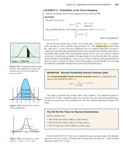s 2p 68% of area –3 95% of the area 99.7% of the area –2 –1 0 1 2 3 Figure 7.48 The 68-95-99.7 rule for normal distributions. The mean m represents the average value of the variable x. The standard deviation s measures the “scatter” around the mean. For a normal curve, the mean and standard deviation tell you where most of the probability lies. The rule of thumb, illustrated in Figure 7.48, is this: The 68-95-99.7 Rule for Normal Distributions y 0 = 0.5 = 1 = 2 Figure 7.49 Normal pdf curves with mean m 2 and s 0.5, 1, and 2. x Given a normal curve, • 68% of the area will lie within s of the mean m, • 95% of the area will lie within 2s of the mean m, • 99.7% of the area will lie within 3s of the mean m. Even with the 68-95-99.7 rule, the area under the curve can spread quite a bit, depending on the size of s. Figure 7.49 shows three normal pdfs with mean m 2 and standard deviations equal to 0.5, 1, and 2.
424 Chapter 7 Applications of Definite Integrals EXAMPLE 6 A Telephone Help Line Suppose a telephone help line takes a mean of 2 minutes to answer calls. If the standard deviation is s 0.5, then 68% of the calls are answered in the range of 1.5 to 2.5 minutes and 99.7% of the calls are answered in the range of 0.5 to 3.5 minutes. Now try Exercise 29. 10.3 11 [9, 11.5] by [–1, 2.5] Figure 7.50 The normal pdf for the spinach weights in Example 7. The mean is at the center. EXAMPLE 7 Weights of Spinach Boxes Suppose that frozen spinach boxes marked as “10 ounces” of spinach have a mean weight of 10.3 ounces and a standard deviation of 0.2 ounce. (a) What percentage of all such spinach boxes can be expected to weigh between 10 and 11 ounces? (b) What percentage would we expect to weigh less than 10 ounces? (c) What is the probability that a box weighs exactly 10 ounces? SOLUTION Assuming that some person or machine is trying to pack 10 ounces of spinach into these boxes, we expect that most of the weights will be around 10, with probabilities tailing off for boxes being heavier or lighter. We expect, in other words, that a normal pdf will model these probabilities. First, we define f x using the formula: 1 f x e x10.320.08 . 0.2 2p The graph (Figure 7.50) has the look we are expecting. (a) For an arbitrary box of this spinach, the probability that it weighs between 10 and 11 ounces is the area under the curve from 10 to 11, which is NINT f x, x, 10, 11 0.933. So without doing any more measuring, we can predict that about 93.3% of all such spinach boxes will weigh between 10 and 11 ounces. (b) For the probability that a box weighs less than 10 ounces, we use the entire area under the curve to the left of x 10. The curve actually approaches the x-axis as an asymptote, but you can see from the graph (Figure 7.50) that f x approaches zero quite quickly. Indeed, f 9 is only slightly larger than a billionth. So getting the area from 9 to 10 should do it: NINT f x, x, 9,100.067. We would expect only about 6.7% of the boxes to weigh less than 10 ounces. (c) This would be the integral from 10 to 10, which is zero. This zero probability might seem strange at first, but remember that we are assuming a continuous, unbroken interval of possible spinach weights, and 10 is but one of an infinite number of them. Now try Exercise 31. Quick Review 7.5 (For help, go to Section 5.2.) In Exercises 1–5, find the definite integral by (a) antiderivatives and (b) using NINT. 1. 1 e x dx 2. 1 e x dx a. e 1 b. 1.718 a. 1 (1/e) b. 0.632 0 0 p2 a. 2/2 b. 0.707 3. sin xdx 4. 3 x 2 2 dx 15 p4 0 5. 2 x2 x 3 dx a. (1/3) ln (9/2) b. 0.501 1 1
Page 1 and 2: Chapter7 Applications of Definite I
Page 3 and 4: 380 Chapter 7 Applications of Defin
Page 45: 422 Chapter 7 Applications of Defin

5128_Ch07_pp378-433

You also want an ePaper? Increase the reach of your titles

Delete template?

Save as template?