5128_Ch07_pp378-433

Chapter 7 Overview
Section 7.1 Integral as Net Change 379
By this point it should be apparent that finding the limits of Riemann sums is not just an
intellectual exercise; it is a natural way to calculate mathematical or physical quantities
that appear to be irregular when viewed as a whole, but which can be fragmented into regular
pieces. We calculate values for the regular pieces using known formulas, then sum
them to find a value for the irregular whole. This approach to problem solving was around
for thousands of years before calculus came along, but it was tedious work and the more
accurate you wanted to be the more tedious it became.
With calculus it became possible to get exact answers for these problems with almost
no effort, because in the limit these sums became definite integrals and definite integrals
could be evaluated with antiderivatives. With calculus, the challenge became one of fitting
an integrable function to the situation at hand (the “modeling” step) and then finding an
antiderivative for it.
Today we can finesse the antidifferentiation step (occasionally an insurmountable hurdle
for our predecessors) with programs like NINT, but the modeling step is no less crucial.
Ironically, it is the modeling step that is thousands of years old. Before either calculus
or technology can be of assistance, we must still break down the irregular whole into regular
parts and set up a function to be integrated. We have already seen how the process
works with area, volume, and average value, for example. Now we will focus more closely
on the underlying modeling step: how to set up the function to be integrated.
7.1
What you’ll learn about
• Linear Motion Revisited
• General Strategy
• Consumption Over Time
• Net Change from Data
• Work
. . . and why
The integral is a tool that can be
used to calculate net change and
total accumulation.
Integral As Net Change
Linear Motion Revisited
In many applications, the integral is viewed as net change over time. The classic example
of this kind is distance traveled, a problem we discussed in Chapter 5.
EXAMPLE 1
Interpreting a Velocity Function
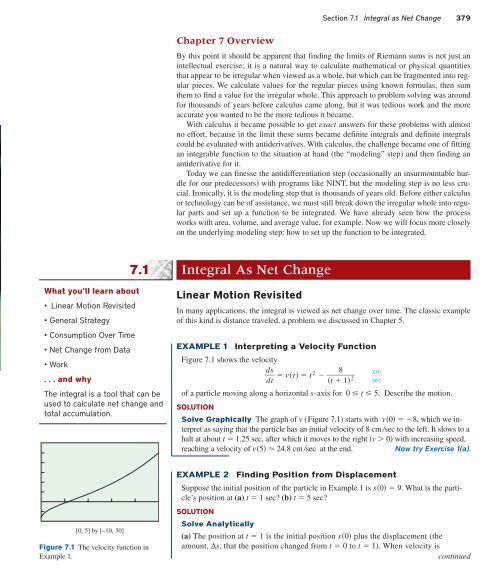
Figure 7.1 shows the velocity
d s
v(t) t
dt
2 c
t
81 2 m s ec
of a particle moving along a horizontal s-axis for 0 t 5. Describe the motion.
SOLUTION
Solve Graphically The graph of v (Figure 7.1) starts with v0 8, which we interpret
as saying that the particle has an initial velocity of 8 cmsec to the left. It slows to a
halt at about t 1.25 sec, after which it moves to the right v 0 with increasing speed,
reaching a velocity of v524.8 cmsec at the end.
Now try Exercise 1(a).
[0, 5] by [–10, 30]
Figure 7.1 The velocity function in
Example 1.
EXAMPLE 2
Finding Position from Displacement
Suppose the initial position of the particle in Example 1 is s0 9. What is the particle’s
position at (a) t 1 sec? (b) t 5 sec?
SOLUTION
Solve Analytically
(a) The position at t 1 is the initial position s0 plus the displacement (the
amount, Δs, that the position changed from t 0 to t 1). When velocity is
continued