5128_Ch03_pp098-184

Section 3.7 Implicit Differentiation 157
3.7
What you’ll learn about
• Implicitly Defined Functions
• Lenses, Tangents, and Normal
Lines
• Derivatives of Higher Order
• Rational Powers of Differentiable
Functions
. . . and why
Implicit differentiation allows us
to find derivatives of functions
that are not defined or written
explicitly as a function of a single
variable.
Implicit Differentiation
Implicitly Defined Functions
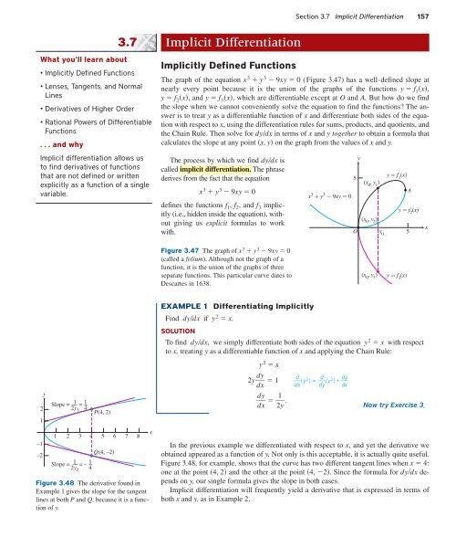
The graph of the equation x 3 y 3 9xy 0 (Figure 3.47) has a well-defined slope at
nearly every point because it is the union of the graphs of the functions y f 1 x,
y f 2 x, and y f 3 x, which are differentiable except at O and A. But how do we find
the slope when we cannot conveniently solve the equation to find the functions? The answer
is to treat y as a differentiable function of x and differentiate both sides of the equation
with respect to x, using the differentiation rules for sums, products, and quotients, and
the Chain Rule. Then solve for dydx in terms of x and y together to obtain a formula that
calculates the slope at any point x, y on the graph from the values of x and y.
The process by which we find dydx is
called implicit differentiation. The phrase
derives from the fact that the equation
x 3 y 3 9xy 0
defines the functions f 1 , f 2 , and f 3 implicitly
(i.e., hidden inside the equation), without
giving us explicit formulas to work
with.
x 3 y 3 9xy 0
5
y
(x 0 , y 1
)
(x 0 , y 2 )
y f 1 (x)
O 5
A
y f 2 (x)
x
x 0
y f 3 (x)
Figure 3.47 The graph of x 3 y 3 9xy 0
(called a folium). Although not the graph of a
function, it is the union of the graphs of three
separate functions. This particular curve dates to
Descartes in 1638.
(x 0 , y 3 )
2
1
–1
–2
y
Slope = –– –
1 =
1 –
2y 1 4
P(4, 2)
1 2 3 4 5 6 7 8
Q(4, –2)
Slope = –– 1 = – 1 –
2y 2 4
Figure 3.48 The derivative found in
Example 1 gives the slope for the tangent
lines at both P and Q, because it is a function
of y.
x
EXAMPLE 1 Differentiating Implicitly
Find dydx if y 2 x.
SOLUTION
To find dydx, we simply differentiate both sides of the equation y 2 x with respect
to x, treating y as a differentiable function of x and applying the Chain Rule:
y 2 x
2y d y
1
dx
d y 1
.
dx
2 y
d
(y 2 d
) = (y 2 ) • d
y
d x d y dx
Now try Exercise 3.
In the previous example we differentiated with respect to x, and yet the derivative we
obtained appeared as a function of y. Not only is this acceptable, it is actually quite useful.
Figure 3.48, for example, shows that the curve has two different tangent lines when x 4:
one at the point 4, 2 and the other at the point 4, 2. Since the formula for dydx depends
on y, our single formula gives the slope in both cases.
Implicit differentiation will frequently yield a derivative that is expressed in terms of
both x and y, as in Example 2.