5128_CH02_58-97

Chapter
2
Limits and
Continuity
58
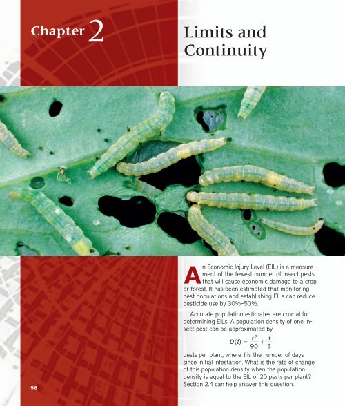
An Economic Injury Level (EIL) is a measurement
of the fewest number of insect pests
that will cause economic damage to a crop
or forest. It has been estimated that monitoring
pest populations and establishing EILs can reduce
pesticide use by 30%–50%.
Accurate population estimates are crucial for
determining EILs. A population density of one insect
pest can be approximated by
t
2
t
D (t) 9 0 3
pests per plant, where t is the number of days
since initial infestation. What is the rate of change
of this population density when the population
density is equal to the EIL of 20 pests per plant?
Section 2.4 can help answer this question.

Chapter 2 Overview
Section 2.1 Rates of Change and Limits 59
The concept of limit is one of the ideas that distinguish calculus from algebra and
trigonometry.
In this chapter, we show how to define and calculate limits of function values. The calculation
rules are straightforward and most of the limits we need can be found by substitution,
graphical investigation, numerical approximation, algebra, or some combination of
these.
One of the uses of limits is to test functions for continuity. Continuous functions arise
frequently in scientific work because they model such an enormous range of natural behavior.
They also have special mathematical properties, not otherwise guaranteed.
2.1
What you’ll learn about
• Average and Instantaneous
Speed
• Definition of Limit
• Properties of Limits
• One-sided and Two-sided
Limits
• Sandwich Theorem
. . . and why
Limits can be used to describe
continuity, the derivative, and the
integral: the ideas giving the
foundation of calculus.
Free Fall
Near the surface of the earth, all bodies
fall with the same constant acceleration.
The distance a body falls after it is released
from rest is a constant multiple
of the square of the time fallen. At least,
that is what happens when a body falls
in a vacuum, where there is no air to
slow it down. The square-of-time rule
also holds for dense, heavy objects like
rocks, ball bearings, and steel tools during
the first few seconds of fall through
air, before the velocity builds up to
where air resistance begins to matter.
When air resistance is absent or insignificant
and the only force acting on
a falling body is the force of gravity, we
call the way the body falls free fall.
Rates of Change and Limits
Average and Instantaneous Speed
A moving body’s average speed during an interval of time is found by dividing the distance
covered by the elapsed time. The unit of measure is length per unit time—kilometers
per hour, feet per second, or whatever is appropriate to the problem at hand.
EXAMPLE 1
Finding an Average Speed
A rock breaks loose from the top of a tall cliff. What is its average speed during the first
2 seconds of fall?
SOLUTION
Experiments show that a dense solid object dropped from rest to fall freely near the surface
of the earth will fall
y 16t 2
feet in the first t seconds. The average speed of the rock over any given time interval is
the distance traveled, y, divided by the length of the interval t. For the first 2 seconds
of fall, from t 0 to t 2, we have
EXAMPLE 2
y
162 2
160 2 ft
32 . Now try Exercise 1.
t
2 0 s ec
Finding an Instantaneous Speed
Find the speed of the rock in Example 1 at the instant t 2.
SOLUTION
Solve Numerically We can calculate the average speed of the rock over the interval
from time t 2 to any slightly later time t 2 h as
y 162 h 2 162
2
. (1)
t
h
We cannot use this formula to calculate the speed at the exact instant t 2 because that
would require taking h 0, and 00 is undefined. However, we can get a good idea of
what is happening at t 2 by evaluating the formula at values of h close to 0. When we
do, we see a clear pattern (Table 2.1 on the next page). As h approaches 0, the average
speed approaches the limiting value 64 ft/sec.
continued

60 Chapter 2 Limits and Continuity
Table 2.1 Average Speeds over
Short Time Intervals Starting at
t 2
y 162 h 2 162
2
t
h
Length of
Average Speed
Time Interval, for Interval
h (sec)
yt (ft/sec)
1 80
0.1 65.6
0.01 64.16
0.001 64.016
0.0001 64.0016
0.00001 64.00016
Confirm Algebraically If we expand the numerator of Equation 1 and simplify, we
find that
y 162 h 2 162 164 4h h 2 64
2
t
h
h
64h 16h
2
64 16h.
h
For values of h different from 0, the expressions on the right and left are equivalent and
the average speed is 64 16h ft/sec. We can now see why the average speed has the
limiting value 64 16(0) 64 ft/sec as h approaches 0. Now try Exercise 3.
Definition of Limit
As in the preceding example, most limits of interest in the real world can be viewed as numerical
limits of values of functions. And this is where a graphing utility and calculus
come in. A calculator can suggest the limits, and calculus can give the mathematics for
confirming the limits analytically.
Limits give us a language for describing how the outputs of a function behave as the
inputs approach some particular value. In Example 2, the average speed was not defined at
h 0 but approached the limit 64 as h approached 0. We were able to see this numerically
and to confirm it algebraically by eliminating h from the denominator. But we cannot always
do that. For instance, we can see both graphically and numerically (Figure 2.1) that
the values of f (x) (sin x)x approach 1 as x approaches 0.
We cannot eliminate the x from the denominator of (sin x)x to confirm the observation
algebraically. We need to use a theorem about limits to make that confirmation, as you will
see in Exercise 75.
X
–.3
–.2
–.1
0
.1
.2
.3
Y1 = sin(X)/X
[–2p, 2p] by [–1, 2]
(a)
Y1
.98507
.99335
.99833
ERROR
.99833
.99335
.98507
(b)
Figure 2.1 (a) A graph and (b) table of
values for f x sin xx that suggest the
limit of f as x approaches 0 is 1.
DEFINITION
Limit
Assume f is defined in a neighborhood of c and let c and L be real numbers. The
function f has limit L as x approaches c if, given any positive number e, there is a
positive number d such that for all x,
0 x c d ⇒ f x L .
We write
lim f x L.
x→c
The sentence lim x→c f x L is read, “The limit of f of x as x approaches c equals L.”
The notation means that the values f (x) of the function f approach or equal L as the values
of x approach (but do not equal) c. Appendix A3 provides practice applying the definition
of limit.
We saw in Example 2 that lim h→0 64 16h 64.
As suggested in Figure 2.1,
lim sin x
1.
x→0 x
Figure 2.2 illustrates the fact that the existence of a limit as x→c never depends on how
the function may or may not be defined at c. The function f has limit 2 as x→1 even though
f is not defined at 1. The function g has limit 2 as x→1 even though g1 2. The function
h is the only one whose limit as x→1 equals its value at x 1.

Section 2.1 Rates of Change and Limits 61
y
y
y
2
2
2
1
1
1
–1 0
1
x
–1 0
1
x
–1 0
1
x
(a) f(x) =
x 2 – 1
x – 1
x 2 – 1 , x ≠ 1
(b) g(x) = x – 1
(c) h(x) = x + 1
1, x = 1
Figure 2.2 lim
x→1
f x lim
x→1
gx lim
x→1
hx 2
Properties of Limits
By applying six basic facts about limits, we can calculate many unfamiliar limits from
limits we already know. For instance, from knowing that
lim k k Limit of the function with constant value k
x→c
and
lim x c, Limit of the identity function at x c
x→c
we can calculate the limits of all polynomial and rational functions. The facts are listed in
Theorem 1.
THEOREM 1 Properties of Limits
If L, M, c, and k are real numbers and
lim f x L and lim gx M, then
x→c x→c
1. Sum Rule: lim f x gx L M
x→c
The limit of the sum of two functions is the sum of their limits.
2. Difference Rule: lim f x gx L M
x→c
The limit of the difference of two functions is the difference of their limits.
3. Product Rule: lim f x • gx L • M
x→c
The limit of a product of two functions is the product of their limits.
4. Constant Multiple Rule: lim k • f x k • L
x→c
The limit of a constant times a function is the constant times the limit of the
function.
f x
L
5. Quotient Rule: lim , M 0
x→c g x
M
The limit of a quotient of two functions is the quotient of their limits, provided
the limit of the denominator is not zero.
continued

62 Chapter 2 Limits and Continuity
6. Power Rule: If r and s are integers, s 0, then
lim f x rs L rs
x→c
provided that L rs is a real number.
The limit of a rational power of a function is that power of the limit of the function,
provided the latter is a real number.
Here are some examples of how Theorem 1 can be used to find limits of polynomial
and rational functions.
EXAMPLE 3
Using Properties of Limits
Use the observations lim x→c k k and lim x→c x c, and the properties of limits to
find the following limits.
(a) lim
x→c
x 3 4x 2 3
SOLUTION
(b) lim x 4 x2
1
x→c x2
5
(a) lim
x→c
x 3 4x 2 3 lim
x→c
x 3 lim
x→c
4x 2 lim
x→c
3
c 3 4c 2 3
(b) lim x4 x2
1 lim
4
x
2
1
x→c x2
x→c
5 lim x2
5
x→
x
c
lim x 4 lim x 2 lim 1
x→c x→c x→c
lim x 2 lim 5
x→c x→c
c4 c2
1
c2
5
Sum and Difference Rules
Product and Constant
Multiple Rules
Quotient Rule
Sum and Difference Rules
Product Rule
Now try Exercises 5 and 6.
Example 3 shows the remarkable strength of Theorem 1. From the two simple observations
that lim x→c k k and lim x→c x c, we can immediately work our way to limits of
polynomial functions and most rational functions using substitution.
THEOREM 2
Polynomial and Rational Functions
1. If f x a n x n a n1 x n1 … a 0 is any polynomial function and c is any
real number, then
lim f x f c a n c n a n1 c n1 … a 0 .
x→c
2. If f x and g(x) are polynomials and c is any real number, then
f x
f c
lim , provided that gc 0.
x→c g x
g c

Section 2.1 Rates of Change and Limits 63
EXAMPLE 4 Using Theorem 2
(a) lim x 2 2 x 3 2 2 3 9
x→3
(b) lim x2 2x 4
22 22
x→2 x 2
2
4
2
1 2
4 3
Now try Exercises 9 and 11.
As with polynomials, limits of many familiar functions can be found by substitution at
points where they are defined. This includes trigonometric functions, exponential and logarithmic
functions, and composites of these functions. Feel free to use these properties.
EXAMPLE 5 Using the Product Rule
Determine lim tan x
.
x→0 x
[–p, p] by [–3, 3]
Figure 2.3 The graph of
f x tan xx
suggests that f x→1 as x→0. (Example 5)
SOLUTION
Solve Graphically The graph of f x tan xx in Figure 2.3 suggests that the limit
exists and is about 1.
Confirm Analytically Using the analytic result of Exercise 75, we have
lim tan x
lim
x→0 x x→0 ( sin x 1
sin
•
x co s
)
tan x =
x
x
c os
x
lim sin x 1
• lim
Product Rule
x→0 x x→0 co s x
1
1 • 1 • 1 co s0 1 1. Now try Exercise 27.
Sometimes we can use a graph to discover that limits do not exist, as illustrated by
Example 6.
[–10, 10] by [–100, 100]
Figure 2.4 The graph of
f (x) (x 3 1x 2)
obtained using parametric graphing to produce
a more accurate graph. (Example 6)
EXAMPLE 6
Use a graph to show that
does not exist.
SOLUTION
Exploring a Nonexistent Limit
lim x 3
1
x→2 x 2
Notice that the denominator is 0 when x is replaced by 2, so we cannot use substitution
to determine the limit. The graph in Figure 2.4 of f (x) (x 3 1x 2) strongly suggests
that as x→2 from either side, the absolute values of the function values get very
large. This, in turn, suggests that the limit does not exist.
Now try Exercise 29.
One-sided and Two-sided Limits
Sometimes the values of a function f tend to different limits as x approaches a number c
from opposite sides. When this happens, we call the limit of f as x approaches c from the

64 Chapter 2 Limits and Continuity
y
4
3
2
y = int x
right the right-hand limit of f at c and the limit as x approaches c from the left the lefthand
limit of f at c. Here is the notation we use:
right-hand:
left-hand:
lim f x
x→c
lim f x
x→c
The limit of f as x approaches c from the right.
The limit of f as x approaches c from the left.
1
–1 1 2 3 4
x
EXAMPLE 7 Function Values Approach Two Numbers
The greatest integer function f (x) int x has different right-hand and left-hand limits at
each integer, as we can see in Figure 2.5. For example,
–2
Figure 2.5 At each integer, the greatest
integer function y int x has different
right-hand and left-hand limits.
(Example 7)
lim int x 3 and lim int x 2.
x→3 x→3 The limit of int x as x approaches an integer n from the right is n, while the limit as x approaches
n from the left is n – 1.
Now try Exercises 31 and 32.
We sometimes call lim x→c f x the two-sided limit of f at c to distinguish it from the
one-sided right-hand and left-hand limits of f at c. Theorem 3 shows how these limits are
related.
On the Far Side
If f is not defined to the left of x c,
then f does not have a left-hand limit at
c. Similarly, if f is not defined to the
right of x c, then f does not have a
right-hand limit at c.
THEOREM 3
One-sided and Two-sided Limits
A function f(x) has a limit as x approaches c if and only if the right-hand and lefthand
limits at c exist and are equal. In symbols,
lim f x L ⇔ lim
x→c x→c
f x L and lim f x L.
x→c 2
1
y
0 1 2 3 4
y = f(x)
Figure 2.6 The graph of the function
x 1, 0 x 1
1, 1 x 2
f x {2, x 2
x 1, 2 x 3
x 5, 3 x 4.
(Example 8)
x
Thus, the greatest integer function f (x) int x of Example 7 does not have a limit as
x→3 even though each one-sided limit exists.
EXAMPLE 8
Exploring Right- and Left-Hand Limits
All the following statements about the function y f (x) graphed in Figure 2.6 are true.
At x 0: lim f x 1.
x→0
At x 1:
At x 2:
At x 3:
lim f x 0 even though f 1 1,
x→1
lim f x 1,
x→1
f has no limit as x→1. (The right- and left-hand limits at 1 are not equal, so
lim x→1 f x does not exist.)
lim f x 1,
x→2
lim f x 1,
x→2 lim f x 1 even though f 2 2.
x→2
lim
x→3
f x lim f x 2 f 3 lim f x.
x→3 x→3
At x 4: lim f x 1.
x→4
At noninteger values of c between 0 and 4, f has a limit as x→c.
Now try Exercise 37.

Section 2.1 Rates of Change and Limits 65
L
y
g
h
f
Sandwich Theorem
If we cannot find a limit directly, we may be able to find it indirectly with the Sandwich
Theorem. The theorem refers to a function f whose values are sandwiched between the
values of two other functions, g and h. If g and h have the same limit as x→c, then f has
that limit too, as suggested by Figure 2.7.
O
Figure 2.7 Sandwiching f between g
and h forces the limiting value of f to be
between the limiting values of g and h.
c
x
THEOREM 4
The Sandwich Theorem
If gx f x hx for all x c in some interval about c, and
lim gx lim hx L,
x→c x→c
then
lim f x L.
x→c
EXAMPLE 9
Show that lim
x→0
x 2 sin 1x 0.
SOLUTION
Using the Sandwich Theorem
We know that the values of the sine function lie between –1 and 1. So, it follows that
x2 sin 1 x x2 •
sin 1 x x2 • 1 x 2
and
x 2 x 2 sin 1 x x2 .
[–0.2, 0.2] by [–0.02, 0.02]
Figure 2.8 The graphs of y 1 x 2 ,
y 2 x 2 sin 1x, and y 3 x 2 . Notice
that y 3 y 2 y 1 . (Example 9)
Because lim
x→0
x 2 lim
x→0
x 2 0, the Sandwich Theorem gives
lim
x→0 (
The graphs in Figure 2.8 support this result.
x2 sin 1 x ) 0.
Quick Review 2.1 (For help, go to Section 1.2.)
In Exercises 1–4, find f(2).
In Exercises 5–8, write the inequality in the form a x b.
1. f x 2x 3 5x 2 4 0
5. x 4 4 x 4
2. f x 4 x2
5
x3
1 6. x c
1
2 c 2 x c 2
4 12
7. x 2 3 1 x 5
8. x c d
3. f x sin ( p x
2 ) 2 c d 2 x c d 2
0
In Exercises 9 and 10, write the fraction in reduced form.
9. x2 3x
18
x 6
3x 1, x 2
x 3
4. f x 1
{ x
2
, x 2 1 1
3 2x
10. 2 x x
2x
2
x 1 x 1

66 Chapter 2 Limits and Continuity
Section 2.1 Exercises
In Exercises 1–4, an object dropped from rest from the top of a tall
building falls y 16t 2 feet in the first t seconds.
1. Find the average speed during the first 3 seconds of fall. 48 ft/sec
2. Find the average speed during the first 4 seconds of fall. 64 ft/sec
3. Find the speed of the object at t 3 seconds and confirm your
answer algebraically. 96 ft/sec
4. Find the speed of the object at t 4 seconds and confirm your
answer algebraically. 128 ft/sec
In Exercises 5 and 6, use lim x→c k k, lim x→c x c, and the properties
of limits to find the limit.
5. lim (2x 3 3x 2 x 1) 2c 3 3c 2 c 1
x→c
6. lim x4
x→c x
x
3 1
2 c4
9 c
c
3 1
2
9
In Exercises 7–14, determine the limit by substitution. Support graphically.
7. lim
x→12 3x2 2x 1 3 8. lim
2 x x→4 31998 1
9. lim x 3 3x 2 2x 1715 10. lim y2 5y 6
5
x→1 y→2 y 2
4y
3
11. lim
y→3 y2 y 2 0
3
12. lim
x→12 int x 0
13. lim
x→2 x 623 4 14. lim
x→2
x 3
In Exercises 15–18, explain why you cannot use substitution to determine
the limit. Find the limit if it exists.
Expression not
15. lim x 2
16. lim 1 Expression not defined at
defined at
x→2 x→0 x2
x 0. There is no limit.
x 2. There
x is no limit.
17. lim
18. lim 4 x 2 16 Expression not
x→0 x
x→0 x
defined at x 0.
Limit 8.
Expression not defined at x 0. There is no limit.
In Exercises 19–28, determine the limit graphically. Confirm algebraically.
1
19. lim
x→1 x
x2
1 20. lim
1 2 t 2 3t 2
t→2 t 2 1 4 4
5x3
8x2
21. lim
x→0 3 x4
16x2
1 2
23. lim 2 x 3 8
12
x→0 x
sin
x
25. lim
x→0 2x
2 1
x
22. lim
x→0
24. lim sin 2x
2
x→0 x
5
1
1 2 x 2
x
26. lim x sin x
2
x→0 x
27. lim sin2 x
0 28. lim 3 sin
4x
4
x→0 x
x→0 sin
3x
1 4
In Exercises 29 and 30, use a graph to show that the limit does not
exist.
29. lim x 2
4
x 1
30. lim
x→1 x 1
x→2 x
2
4
In Exercises 31–36, determine the limit.
31. lim int x 0 32. lim int x 1
x→0 x→0
33. lim int x 0 34. lim int x 1
x→0.01 x→2
35. lim x
1 36. lim x
1
x→0 x
x→0 x
In Exercises 37 and 38, which of the statements are true about the
function y f (x) graphed there, and which are false?
37.
38.
(a) lim f x 1 True (b) lim f x 0
x→1 x→0
(c) lim
x→0
f x 1 False (d) lim
x→0
(e) lim
x→0
f x exists True (f) lim
x→0
f x 0
(g) lim
x→0
f x 1 False (h) lim
x→1
f x 1
(i) lim
x→1
f x 0 False (j)lim
x→2 f x 2
–1
x→0
True
f x lim f x True
True
False
False
(a) lim f x 1 True (b) lim f x does not exist. False
x→1 x→2
(c) lim
x→2
f x 2 False (d) lim
x→1 f x 2
(e) lim
x→1
1
2
1
0
y
–1 0 1
y
True
f x 1 True (f) lim f x does not exist. True
x→1
(g) lim f x lim f x
x→0 x→0
1
y = f(x)
y f(x)
True
(h) lim
x→c
f x exists at every c in 1, 1.
(i) lim
x→c
f x exists at every c in 1, 3.
29. Answers will vary. One possible graph is given by the window [4.7, 4.7] by [15, 15] with Xscl 1 and Yscl 5.
30. Answers will vary. One possible graph is given by the window [4.7, 4.7] by [15, 15] with Xscl 1 and Yscl 5.
2
2
x
3
x
True
True

Section 2.1 Rates of Change and Limits 67
In Exercises 39–44, use the graph to estimate the limits and value of
the function, or explain why the limits do not exist.
39. y
(a) lim f x 3
x→3
(b) lim
x→3 f x
(c) lim
x→3
f x
(d) f 3 1
2
No limit
40. y
(a) lim gt 5
t→4
(b) lim
t→4 gt 2
(c) lim
t→4
gt
(d) g4 2
41. y
(a) lim f h
h→0
y = f(h)
(b) lim
h→0 f h
(c) lim
h→0
f h
(d) f 0
4
42. y
(a) lim ps 3
s→2
–2
(b) lim
s→2 ps 3
(c) lim
s→2 ps 3
(d) p2 3
43. y
(a) lim Fx 4
x→0
4
(b) lim
x→0 Fx
(c) lim
x→0
Fx
(d) F0 4
44. y
(a) lim Gx 1
x→2
y = G(x)
–4
2
y = f(x)
3 x
y = g(t)
y = p(s)
y = F(x)
2
s
x
x
t
h
No limit
4
4
4
3
(b) lim
x→2 Gx 1
(c) lim
x→2
Gx 1
(d) G2 3
No limit
In Exercises 45–48, match the function with the table.
45. y 1 x2 x 2
(c) 46. y
x 1
1 x2 x 2
(b)
x 1
47. y 1 x2 2x 1
(d)
x 1
48. y 1 x2 x 2
(a)
x 1
In Exercises 49 and 50, determine the limit.
49. Assume that lim f x 0 and lim gx 3.
x→4 x→4
(a) lim gx 3 6 (b) lim x f x 0
x→4 x→4
(c) lim g 2 x
x 9 (d) lim
x→4 x→4 f x
g 1
50. Assume that lim
x→b
f x 7 and lim
x→b
gx 3.
3
(a) lim
x→b
f x gx 4 (b) lim
x→b
f x • gx 21
(c) lim
x→b
4 gx 12
f x
(d) lim
x→b g x
In Exercises 51–54, complete parts (a), (b), and (c) for the piecewisedefined
function.
(a) Draw the graph of f.
(b) Determine lim x→c f x and lim x→c f x.
(c) Writing to Learn Does lim x→c f x exist? If so, what is it?
If not, explain.
3 x, x 2 (b) Right-hand: 2 Left-hand: 1
51. c 2, f x x (c) No, because the two one-sided
{ 1, x 2 limits are different.
2
3 x, x 2
52. c 2, f x
{ 2, x 2
x2, x 2
{
1
53. c 1, f x x 1
x
54.
X
.7
.8
.9
1
1.1
1.2
1.3
X = .7
X
.7
.8
.9
1
1.1
1.2
1.3
X = .7
Y1
–.4765
–.3111
–.1526
0
.14762
.29091
.43043
Y1
(a)
2.7
2.8
2.9
ERROR
3.1
3.2
3.3
(c)
, x 1
3 2x 5, x 1
1 x 2 , x 1
c 1, f x { 2, x 1
X
.7
.8
.9
1
1.1
1.2
1.3
X = .7
X
.7
.8
.9
1
1.1
1.2
1.3
X = .7
Y1
7.3667
10.8
20.9
ERROR
–18.9
–8.8
–5.367
Y1
(b)
–.3
–.2
–.1
ERROR
.1
.2
.3
(d)
7 3
(b) Right-hand: 1 Left-hand: 1
(c) Yes. The limit is 1.
(b) Right-hand: 4 Left-hand:
no limit (c) No, because the
left-hand limit doesn’t exist.
(b) Right-hand: 0 Left-hand: 0
(c) Yes. The limit is 0.

68 Chapter 2 Limits and Continuity
In Exercises 55–58, complete parts (a)–(d) for the piecewise-defined
function.
(a) Draw the graph of f.
(b) At what points c in the domain of f does lim x→c f x exist?
(c) At what points c does only the left-hand limit exist?
(d) At what points c does only the right-hand limit exist?
55.
56.
57.
58.
sin x, 2p x 0
f x { cos x, 0 x 2p
cos x, p x 0
f x { sec x, 0 x p
1 x 2 , 0 x 1
f x
{ 1, 1 x 2
2, x 2
x, 1 x 0, or 0 x 1
f x
{ 1, x 0
0, x 1, or x 1
In Exercises 59–62, find the limit graphically. Use the Sandwich
Theorem to confirm your answer.
59. lim x sin x 0 60. lim x 2 sin x 0
x→0 x→0
61. lim
x→0
x 2 sin x
1
2 0 62. lim
x→0
x 2 cos x
1
2 0
63. Free Fall A water balloon dropped from a window high above
the ground falls y 4.9t 2 m in t sec. Find the balloon’s
(a) average speed during the first 3 sec of fall. 14.7 m/sec
(b) speed at the instant t 3.
29.4 m/sec
64. Free Fall on a Small Airless Planet A rock released from
rest to fall on a small airless planet falls y gt 2 m in t sec, g a
constant. Suppose that the rock falls to the bottom of a crevasse
20 m below and reaches the bottom in 4 sec.
(a) Find the value of g. g 5 4
(b) Find the average speed for the fall. 5 m/sec
(c) With what speed did the rock hit the bottom?
66. True.
lim
x→0 x sin x
x
lim
x→0 1 sin x
x
1 lim sin x
2
x→0 x
Standardized Test Questions
(b) (2p, 0) (0, 2p)
(c) c 2p (d) c 2p
(b)
p, p 2 p 2 , p
(c) c p
(d) c p
(b) (0, 1) (1, 2)
(c) c 2 (d) c 0
(b) (, 1) (1, 1) (1, )
(c) None (d) None
10 m/sec
You should solve the following problems without using a
graphing calculator.
65. True or False If lim f (x) 2 and lim f (x) 2, then
x→c x→c
lim f (x) 2. Justify your answer. True. Definition of limit.
x→c
66. True or False lim x sin x
2. Justify your answer.
x→0 x
In Exercises 67–70, use the following function.
2 x, x 1
f x x
{ 1, x 1
2
67. Multiple Choice What is the value of lim f (x)? C
x→1
(A) 52 (B) 32 (C) 1 (D) 0 (E) does not exist
68. Multiple Choice What is the value of lim x→1 f (x)? B
(A) 52 (B) 32 (C) 1 (D) 0 (E) does not exist
69. Multiple Choice What is the value of lim x→1 f (x)? E
(A) 52 (B) 32 (C) 1 (D) 0 (E) does not exist
70. Multiple Choice What is the value of f (1)? C
(A) 52 (B) 32 (C) 1 (D) 0 (E) does not exist
Explorations
In Exercises 71–74, complete the following tables and state what you
believe lim x→0 f (x) to be.
(a)
x 0.1 0.01 0.001 0.0001 …
f x ? ? ? ?
(b)
x 0.1 0.01 0.001 0.0001 …
f x ? ? ? ?
71. f x x sin 1 x 72. f x sin 1 x
73. f x 10 x 1
74. f x x sin ln x
x
75. Group Activity To prove that lim u→0 (sin u)u 1 when u is
measured in radians, the plan is to show that the right- and lefthand
limits are both 1.
(a) To show that the right-hand limit is 1, explain why we can
restrict our attention to 0 u p2. Because the right-hand limit at
zero depends only on the values of the function for positive x-values near zero.
(b) Use the figure to show that
1
O
area of OAP 1 sin u,
2
area of sector OAP u 2 ,
area of OAT 1 tan u.
2
y
⎧
⎪⎪⎪⎪⎪⎨⎪⎪⎪⎪⎪⎩
(c) Use part (b) and the figure to show that for 0 u p2,
1 2 sin u 1 2 u 1 tan u.
2
This is how the areas of the three regions compare.
1
cos
1
sin
P
Q
T
tan
A(1, 0)
Use: area of triangle
1 2 (base)(height)
area of circular sector
(angle)( radius)
2
2
x

Section 2.1 Rates of Change and Limits 69
(d) Show that for 0 u p2 the inequality of part (c) can be
written in the form
u 1 Multiply by 2 and divide
1 .
sin u co s u by sin u.
(e) Show that for 0 u p2 the inequality of part (d) can be
written in the form
cos u sin Take reciprocals, remembering
u
1. that all of the values involved
u are positive.
(f) Use the Sandwich Theorem to show that
lim sin u
1.
u→0 u
(g) Show that sin uu is an even function.
(h) Use part (g) to show that
lim sin u
1.
u→0 u
(i) Finally, show that
lim sin u
1. The two one-sided limits both
u→0 u exist and are equal to 1.
Extending the Ideas
76. Controlling Outputs Let f x 3x 2.
The limit can be found by
(a) Show that lim x→2 f x 2 f 2.
substitution.
(b) Use a graph to estimate values for a and b so that
1.8 f (x) 2.2 provided a x b. One possible answer:
a 1.75, b 2.28
(c) Use a graph to estimate values for a and b so that
1.99 f (x) 2.01 provided a x b. One possible answer:
a 1.99, b 2.01
77. Controlling Outputs Let f (x) sin x.
(a) Find f p6. f p 6 1 2
(b) Use a graph to estimate an interval (a, b) about x p6 so
that 0.3 f (x) 0.7 provided a x b. One possible answer:
a 0.305, b 0.775
(c) Use a graph to estimate an interval (a, b) about x p6 so
that 0.49 f (x) 0.51 provided a x b. One possible answer:
a 0.513, b 0.535
78. Limits and Geometry Let P(a, a 2 ) be a point on the parabola
y x 2 , a 0. Let O be the origin and (0, b) the y-intercept of the
perpendicular bisector of line segment OP. Find lim P→O b. 1 2
75. (f) The limits for cos u and 1 are both equal to 1. Since sin u
is between
u
them, it must also have a limit of 1.
(g) sin (
u)
u
s in
(u)
u
sin (u)
u
(h) If the function is symmetric about the y-axis, and the right-hand limit at
zero is 1, then the left-hand limit at zero must also be 1.

70 Chapter 2 Limits and Continuity
2.2
What you’ll learn about
•Finite Limits as x→
• Sandwich Theorem Revisited
•Infinite Limits as x→a
• End Behavior Models
• “Seeing” Limits as x→
. . . and why
Limits can be used to describe
the behavior of functions for
numbers large in absolute value.
Limits Involving Infinity
Finite Limits as x:
The symbol for infinity () does not represent a real number. We use to describe the behavior
of a function when the values in its domain or range outgrow all finite bounds. For
example, when we say “the limit of f as x approaches infinity” we mean the limit of f as x
moves increasingly far to the right on the number line. When we say “the limit of f as x approaches
negative infinity ()” we mean the limit of f as x moves increasingly far to the
left. (The limit in each case may or may not exist.)
Looking at f x 1x (Figure 2.9), we observe
(a) as x→, 1x→0 and we write
lim 1x 0,
x→
(b) as x→, 1x→0 and we write
lim 1x 0.
x→
We say that the line y 0 is a horizontal asymptote of the graph of f.
[–6, 6] by [–4, 4]
Figure 2.9 The graph of f (x) 1x
0
1
2
3
4
5
6
X
[–10, 10] by [–1.5, 1.5]
(a)
Y1
0
.7071
.8944
.9487
.9701
.9806
.9864
Y1 = X/√ (X 2 + 1)
X
- 6
- 5
- 4
- 3
- 2
- 1
0
Y1
- .9864
- .9806
- .9701
- .9487
- .8944
- .7071
0
Y1 = X/√ (X 2 + 1)
(b)
Figure 2.10 (a) The graph of f x
xx 2 1 has two horizontal asymptotes,
y 1 and y 1. (b) Selected
values of f. (Example 1)
DEFINITION
Horizontal Asymptote
The line y b is a horizontal asymptote of the graph of a function y f(x) if either
The graph of f x 2 (1x) has the single horizontal asymptote y 2 because
lim
x→
( 2 1 x ) 2 and lim
x→
( 2 1 x ) 2.
A function can have more than one horizontal asymptote, as Example 1 demonstrates.
EXAMPLE 1 Looking for Horizontal Asymptotes
Use graphs and tables to find lim x→ f (x), lim x→ f (x), and identify all horizontal
asymptotes of f (x) xx 2 1.
lim f x b or lim f x b.
x→
x→
SOLUTION
Solve Graphically Figure 2.10a shows the graph for 10 x 10. The graph
climbs rapidly toward the line y 1 as x moves away from the origin to the right.
On our calculator screen, the graph soon becomes indistinguishable from the line.
Thus lim x→ f (x) 1. Similarly, as x moves away from the origin to the left, the
graph drops rapidly toward the line y 1 and soon appears to overlap the line. Thus
lim x→ f (x) 1. The horizontal asymptotes are y 1 and y 1.
continued

Section 2.2 Limits Involving Infinity 71
Confirm Numerically The table in Figure 2.10b confirms the rapid approach of f (x)
toward 1 as x→. Since f is an odd function of x, we can expect its values to approach
1 in a similar way as x→. Now try Exercise 5.
Sandwich Theorem Revisited
The Sandwich Theorem also holds for limits as x→.
X
100
200
300
400
500
600
700
[–4, 4] by [–0.5, 1.5]
Y1
Y1 = sin(X)/X
(a)
–.0051
–.0044
–.0033
–.0021
–9E–4
7.4E–5
7.8E–4
(b)
Figure 2.11 (a) The graph of f x
sin xx oscillates about the x-axis. The
amplitude of the oscillations decreases
toward zero as x→. (b) A table of values
for f that suggests f x→0 as x→.
(Example 2)
EXAMPLE 2 Finding a Limit as x Approaches
Find lim f x for f x sin x
.
x→ x
SOLUTION
Solve Graphically and Numerically The graph and table of values in Figure 2.11
suggest that y 0 is the horizontal asymptote of f.
Confirm Analytically We know that 1 sin x 1. So, for x 0 we have
1 x sin x
1 x x .
Therefore, by the Sandwich Theorem,
0 lim
x→ ( 1 x ) lim sin x
lim 1
x→ x x→ x 0.
Since sin xx is an even function of x, we can also conclude that
lim sin x
0. Now try Exercise 9.
x→ x
Limits at infinity have properties similar to those of finite limits.
THEOREM 5
Properties of Limits as x→
If L, M, and k are real numbers and
lim f x L
x→
and lim gx M, then
x→
1. Sum Rule: lim f x gx L M
x→
2. Difference Rule: lim f x gx L M
x→
3. Product Rule: lim f x • gx L • M
x→
4. Constant Multiple Rule: lim k • f x k • L
x→
5. Quotient Rule: lim f x
L
, M 0
x→ gx
M
6. Power Rule: If r and s are integers, s 0, then
lim f
x→ xrs L rs
provided that
L r>s
is a real number.

72 Chapter 2 Limits and Continuity
We can use Theorem 5 to find limits at infinity of functions with complicated expressions,
as illustrated in Example 3.
EXAMPLE 3 Using Theorem 5
Find lim 5x sin x
.
x→ x
SOLUTION
Notice that
So,
5x sin x
5 x
sin x
5 sin x
.
x x x x
lim 5x sin x
lim 5 lim sin x
x→ x x→ x→ x
5 0 5.
Sum Rule
Known Values
Now try Exercise 25.
EXPLORATION 1
Exploring Theorem 5
We must be careful how we apply Theorem 5.
1. (Example 3 again) Let f (x) 5x sin x and g(x) x. Do the limits as x→
of f and g exist? Can we apply the Quotient Rule to lim x→ f xgx? Explain.
Does the limit of the quotient exist?
2. Let f (x) sin 2 x and g(x) cos 2 x. Describe the behavior of f and g as x→.
Can we apply the Sum Rule to lim x→ f x gx? Explain. Does the limit of
the sum exist?
3. Let f (x) ln (2x) and g(x) ln (x 1). Find the limits as x→ of f and g. Can
we apply the Difference Rule to lim x→ f x gx? Explain. Does the limit
of the difference exist?
4. Based on parts 1–3, what advice might you give about applying Theorem 5?
Infinite Limits as x→a
If the values of a function f (x) outgrow all positive bounds as x approaches a finite number
a, we say that lim x→a f x . If the values of f become large and negative, exceeding all
negative bounds as x→a, we say that lim x→a f x .
Looking at f (x) 1x (Figure 2.9, page 70), we observe that
lim 1x and lim 1x .
x→0 x→0 We say that the line x 0 is a vertical asymptote of the graph of f.
DEFINITION
Vertical Asymptote
The line x a is a vertical asymptote of the graph of a function y f (x) if either
lim
x→a
x→a
f x or lim f x

Section 2.2 Limits Involving Infinity 73
. . . , 3 p p ,
2 2 , p 2 , 3 p , . . . . (Example 5) You might think that the graph of a quotient always has a vertical asymptote where the
2
denominator is zero, but that need not be the case. For example, we observed in Section
EXAMPLE 4 Finding Vertical Asymptotes
Find the vertical asymptotes of f x x
12
. Describe the behavior to the left and right of
each vertical asymptote.
SOLUTION
The values of the function approach on either side of x 0.
lim 1
x→0 x2 and lim 1
x→0
x2 .
The line x 0 is the only vertical asymptote. Now try Exercise 27.
We can also say that lim x→0 1x 2 . We can make no such statement about 1x.
EXAMPLE 5 Finding Vertical Asymptotes
The graph of f x tan x sin xcos x has infinitely many vertical asymptotes,
one at each point where the cosine is zero. If a is an odd multiple of p2, then
[–2p, 2p] by [–5, 5]
lim tan x
x→a and lim tan x ,
x→a Figure 2.12 The graph of f (x) tan x
has a vertical asymptote at
as suggested by Figure 2.12. Now try Exercise 31.
2.1 that lim x→0 sin xx 1.
y =3x 4 – 2x 3 + 3x 2 – 5x + 6
End Behavior Models
For numerically large values of x, we can sometimes model the behavior of a complicated
function by a simpler one that acts virtually in the same way.
[–2, 2] by [–5, 20]
(a)
[–20, 20] by [–100000, 500000]
(b)
Figure 2.13 The graphs of f and g,
(a) distinct for x small, are (b) nearly
identical for x large. (Example 6)
EXAMPLE 6
Modeling Functions For ⏐x⏐ Large
Let f (x) 3x 4 2x 3 3x 2 5x 6 and g(x) 3x 4 . Show that while f and g are quite
different for numerically small values of x, they are virtually identical for x large.
SOLUTION
Solve Graphically The graphs of f and g (Figure 2.13a), quite different near the origin,
are virtually identical on a larger scale (Figure 2.13b).
Confirm Analytically We can test the claim that g models f for numerically large
values of x by examining the ratio of the two functions as x→. We find that
lim f x
3x
lim 4 2x3
3x2 5x 6 x→ gx
x→
3x 4
lim
x→ ( 1 2 1 5
3x
x 2 3 x 3 2
x
1,
convincing evidence that f and g behave alike for x large. Now try Exercise 39.
4)

74 Chapter 2 Limits and Continuity
DEFINITION End Behavior Model
The function g is
f x
(a) a right end behavior model for f if and only if lim 1.
x→ g x
(b) a left end behavior model for f if and only if lim f x
1.
x→ gx
If one function provides both a left and right end behavior model, it is simply called an
end behavior model. Thus, g(x) 3x 4 is an end behavior model for f (x) 3x 4 2x 3
3x 2 5x 6 (Example 6).
In general, g(x) a n x n is an end behavior model for the polynomial function f (x)
a n x n a n1 x n 1 … a 0 , a n 0. Overall, the end behavior of all polynomials behave
like the end behavior of monomials. This is the key to the end behavior of rational functions,
as illustrated in Example 7.
EXAMPLE 7
Find an end behavior model for
Finding End Behavior Models
(a) f x 2x5 x 4
3x
2 5
x
2 1
x 7
(b) gx 2 x
5 x
3
3
x2
x 1
x2
x 5
SOLUTION
(a) Notice that 2x 5 is an end behavior model for the numerator of f, and 3x 2 is one
for the denominator. This makes
an end behavior model for f.
2 x5
3x2 2 3 x3
(b) Similarly, 2x 3 is an end behavior model for the numerator of g, and 5x 3 is one for
the denominator of g. This makes
2 x3
5x3 2 5
an end behavior model for g. Now try Exercise 43.
Notice in Example 7b that the end behavior model for g, y 25, is also a horizontal
asymptote of the graph of g, while in 7a, the graph of f does not have a horizontal asymptote.
We can use the end behavior model of a rational function to identify any horizontal
asymptote.
We can see from Example 7 that a rational function always has a simple power function
as an end behavior model.
A function’s right and left end behavior models need not be the same function.
EXAMPLE 8 Finding End Behavior Models
Let f (x) x e x . Show that g(x) x is a right end behavior model for f while
h(x) e x is a left end behavior model for f.
SOLUTION
On the right,
lim
x→ f x
lim x e
x
lim
gx
x→ x x→ ( 1 x
x
e 1 because lim
x
x→ e 0.
x
)
continued

Section 2.2 Limits Involving Infinity 75
On the left,
lim f x
lim
x→ hx
x ex
x→ e x
lim
x→ ( x
e x 1)
1 because lim x
x→ e x 0.
The graph of f in Figure 2.14 supports these end behavior conclusions.
Now try Exercise 45.
[–9, 9] by [–2, 10]
Figure 2.14 The graph of f (x) x e x
looks like the graph of g(x) x to the right
of the y-axis, and like the graph of h(x)
e x to the left of the y-axis. (Example 8)
“Seeing” Limits as x→
We can investigate the graph of y f (x) as x→ by investigating the graph of
y f 1x as x→0.
EXAMPLE 9
Find lim
x→
sin 1x.
SOLUTION
Using Substitution
Figure 2.15a suggests that the limit is 0. Indeed, replacing lim x→ sin 1x by the
equivalent lim x→0 sin x 0 (Figure 2.15b), we find
lim
x→
sin 1x lim sin x 0. .
x→0 Now try Exercise 49.
[–10, 10] by [–1, 1]
(a)
[–2p, 2p] by [–2, 2]
(b)
Figure 2.15 The graphs of (a) f x sin 1x and (b) gx f 1x sin x. (Example 9)
5. q(x) 2 3
6. q(x) 2x 2 2x 1
r(x) 3x 2 5 3 x 7 3 r(x) x 2 x 2
Quick Review 2.2 (For help, go to Section 1.2 and 1.5.)
In Exercises 1–4, find f 1 and graph f, f 1 , and y x in the same
square viewing window.
1. f x 2x 3 f 1 (x) x 3
2. f x e x f 1 (x) ln (x)
2
3. f (x) tan 1 x 4. f(x) cot 1 x
f 1 (x) tan (x), p 2 x p 2 f 1 (x) cot (x), 0 x p
In Exercises 5 and 6, find the quotient q(x) and remainder r(x) when
f (x) is divided by g(x).
5. f (x) 2x 3 3x 2 x 1, g(x) 3x 3 4x 5
6. f (x) 2x 5 x 3 x 1, g(x) x 3 x 2 1
In Exercises 7–10, write a formula for (a) f(x) and (b) f(1x). Simplify
where possible.
7. f (x) cos x (a) f(x) cos x (b) f 1 x cos 1 x
8. f (x) e x (a) f(x) e x (b) f
1 x e1/x
9. f x ln x
x
10. f x x 1 x sin x
(a) f(x) ln ( x)
x
(a) f(x)
x 1 x sin x
(b) f
1 x
x ln x
(b) f 1 x 1 x x sin 1 x

76 Chapter 2 Limits and Continuity
Section 2.2 Exercises
In Exercises 1–8, use graphs and tables to find (a) lim x→ f x and
(b) lim x→ f x (c) Identify all horizontal asymptotes.
(a) 1 (b) 1
1. f x cos
( 1 x ) 2. f x sin (c) y 1
x
2x
(a) 0 (b) 0
(c) y 0
3. f x e x
(a) 0 (b)
4. f x 3x3 x 1
(a) (b)
x (c) y 0
x 3 (c) None
3x
1 (a) 3 (b) 3
2x
5. f x 6. f x
1 (a) 2 (b) 2
x
2 (c) y 3, y 3 x
3 (c) y 2, y 2
x (a) 1 (b) 1
x
7. f x
8. f x (a) 1 (b) 1 (c) y 1
x (c) y l, y l x 1
(a)
(b)
In Exercises 9–12, find the limit and confirm your answer using the
Sandwich Theorem.
9. lim 1 cos x
0
10. lim
x→ x2
1 cos x
0
x→ x2
11. lim sin x
0 12. lim sin (x 2 )
0
x→ x
x→ x
In Exercises 13–20, use graphs and tables to find the limits.
13. lim 1
14. lim
x→2
x 2
x
x→2
x 2
15. lim 1
16. lim
x→3 x 3
x
x→3 x 3
17. lim t x
x→0
x 0 18. lim t x
x→0
x
19. lim csc x 20. lim sec x
x→0 x→p2
In Exercises 21–26, find lim x→ y and lim x→ y.
Both are 5
21. y ( 2 x
x
)( 1
x 2
5
) x 2 22. y ( 2 x )( 1 1
5x2 x
) 2
Both are 1
cos 1x
23. y Both are 1 24. y 2x sin x
Both are 2
1 1x
x
sin
x
25. y 2x
2 Both are 0 26. y x sin x 2 sin x
x
2x 2 Both are 0
In Exercises 27–34, (a) find the vertical asymptotes of the graph of
f (x). (b) Describe the behavior of f (x) to the left and right of each
vertical asymptote.
1 (a) x 2, x 2
x
27. f x x
2
28. f x 2 1
(a) x 2
4
2 x 4
29. f x x2 2x
1 x (a) x 1 (a) x 1 30. f x
x 1
2x
2
2 , x 3
5x 3
31. f x cot x (a) x kp, k any 32. f x sec x (a) x p 2 np,
33. f (x) t integer
an
x
co
34. f (x) t
x n any integer
sin
x
c os
x
In Exercises 35–38, match the function with the graph of its end behavior
model.
35. y 2x3 3x
x
2 1
3
(a) 36. y x5
2 x
x
4 x 1
2 (c)
x 3
37. y 2x4 x 3 x 2 1
(d) 38. y x4 3x
3 x 2 1
2 x
1 x 2 (b)
In Exercises 39–44, (a) find a power function end behavior model for
f. (b) Identify any horizontal asymptotes.
39. f (x) 3x 2 2x 1 40. f (x) 4x 3 x 2 2x 1
(a) 3x 2 (b) None
(a) 4x 3 (b) None
x 2
41. f x 2x
2
42. f x 3x2 x 5
3x 5
x
1
4
(a) (b) y 0
(a) 3 (b) y 3
2 x
43. f x 4x3 2x 1
x
44. f x
2x 2 x 3
(a) 4x 2 (b) None
x 2
x 2 4
(a) x 2 (b) None
In Exercises 45–48, find (a) a simple basic function as a right end behavior
ln x
51. f x At : 0 At :0 52. f x x sin 1 x At : 1 At :1
x
model and (b) a simple basic function as a left end behavior
model for the function.
45. y e x 2x (a) e x (b) 2x 46. y x 2 e x (a) x 2 (b) e x
47. y x ln x (a) x (b) x 48. y x 2 sin x (a) x 2 (b) x 2
In Exercises 49–52, use the graph of y f 1x to find lim x→ f x
and lim x→ f x.
49. f (x) xe x At : At :0 50. f (x) x 2 e x At : 0 At :
In Exercises 53 and 54, find the limit of f x as (a) x→,
(b) x→, (c) x→0 , and (d) x→0 .
1x, x 0
53. f x {
{
1, x 0 (a) 0 (b) 1 (c) (d) 1
x 2
, x 0
54. f x x 1
1x 2 , x 0 (a) 1 (b) 0 (c) 2 (d)
Group Activity In Exercises 55 and 56, sketch a graph of a function
y f (x) that satisfies the stated conditions. Include any asymptotes.
55. lim
x→1
f x 2,
lim f x 1, lim
x→
lim f x , lim
x→2 56. lim
x→2
f x 1,
lim f x , lim
x→
(c)
lim f x , lim
x→5
f x ,
x→2 f x 0
x→
lim f x , lim
x→4
f x 2
x→
(d)
f x ,
x→5 f x ,
x→4

Section 2.2 Limits Involving Infinity 77
f
57. 1 ( x)
/ f2(
x)
f 1(
x)
/ g1(
x)
f
As x goes to infinity, 1 f
and 2 f
both approach 1. Therefore, using the above equation, 1 f
2
must also approach 1.
g 1(
x)
/ g2(
x)
f2(
x)
/ g2(
x)
g 1 g 2
g 1g2
3
57. Group Activity End Behavior Models Suppose that g 1 (x) (c) f x , gx (x 2)
is a right end behavior model for f 1 (x) and that g 2 (x) is a right
x 2
3 , c 2
f →− as x →2 − , f → as x →2 + , g → 0, fg →0
end behavior model for f 2 (x). Explain why this makes g 1 xg 2 x
5
(d) f x ,
a right end behavior model for f 1 xf 2 x.
(3 x) 4 gx (x 3) 2 , c 3
x→ , g → 0, fg →
58. Writing to Learn Let L be a real number, lim x→c f x L,
and lim x→c gx or . Can lim x→c f x gx be
determined? Explain. x
59. True. For example, f (x) has y 1 as horizontal asymptotes.
x 2
1
Standardized Test Questions
You may use a graphing calculator to solve the following
problems.
59. True or False It is possible for a function to have more than
one horizontal asymptote. Justify your answer.
60. True or False If f (x) has a vertical asymptote at x c, then either
lim x→c f (x) lim x→c f (x) or lim x→c f (x)
lim x→c f (x) . Justify your answer. False. Consider f (x) 1x.
61. Multiple Choice lim x
x→2
A
x 2
(A) (B) (C) 1 (D) 12 (E) 1
62. Multiple Choice lim cos (2x)
E
x→0 x
(A) 12 (B) 1 (C) 2 (D) cos 2 (E) does not exist
63. Multiple Choice lim sin (3x)
C
x→0 x
(A) 13 (B) 1 (C) 3 (D) sin 3 (E) does not exist
64. Multiple Choice Which of the following is an end behavior for
f (x) 2x3 x2
x 1
?
x3
1
(A) x 3 (B) 2x 3 (C) 1x 3 (D) 2 (E) 12
Exploration
65. Exploring Properties of Limits Find the limits of f, g, and fg
as x→c.
(a) f x 1 f → as x →0 − , f → as x →0 + , g → 0, fg →1
, gx x, c 0
x
f → as x →0 − , f →− as x →0 + , g → 0, fg →−8
(b) f x x
23 , gx 4x3 , c 0
(e) Writing to Learn Suppose that lim x→c f x 0 and
lim x→c gx . Based on your observations in parts (a)–(d),
what can you say about lim x→c f x • gx?
Nothing—you need more information to decide.
Extending the Ideas
66. The Greatest Integer Function
This follows from x 1 int x x which is true for all
(a) Show that
x 1
in x. Dividing by x gives the result.
t x x 1
1 x 0 and in t x 1 x 0.
x x
x x
(b) Determine lim in t x . 1
x→ x
(c) Determine lim in t x . 1
x→ x
67. Sandwich Theorem Use the Sandwich Theorem to confirm
the limit as x→ found in Exercise 3.
68. Writing to Learn Explain why there is no value L for which
lim x→ sin x L. This is because as x approaches infinity, sin x continues
to oscillate between 1 and 1 and doesn’t approach any single real number.
In Exercises 69–71, find the limit. Give a convincing argument that
the value is correct.
69. lim l n x2
Limit 2, because l n x2
x→ ln
x
ln
x
2 ln x
ln 2.
x
ln
x
70. lim
x→ l og
x
Quick Quiz for AP* Preparation: Sections 2.1 and 2.2
D
ln
x ln x
Limit ln (10), since ln 10.
l og
x ln x ln10
71. lim ln x 1
x→ ln
x
Limit 1. Since ln (x 1) ln x
1 1 x ln x ln 1 1 x ,ln ( x 1)
ln
x
ln x ln (1 1x)
1 ln (1 1x)
ln
. x
But as x → , 1 + 1 x approaches 1, so
ln x
ln 1 + 1 x
approaches ln (1) 0. Also, as x → , lnx approaches infinity. This
means the second term above approaches 0 and the limit is 1.
58. Yes. The limit of ( f g) will be the same as the limit of g. This is because adding numbers that are very close to a given real number L will not have a significant
effect on the value of ( f g) since the values of g are becoming arbitrarily large.
You should solve the following problems without using
a graphing calculator.
1. Multiple Choice Find lim x2 x 6
, if it exists. D
x→3 x 3
(A) 1 (B) 1 (C) 2 (D) 5 (E) does not exist
2. Multiple Choice Find lim f (x), if it exists, where A
x→2
3x 1, x 2
f x 5
{, x 2
x 1
(A) 53 (B) 133 (C) 7 (D) (E) does not exist
3. Multiple Choice Which of the following lines is a horizontal
asymptote for
f(x) 3x 3
x 2 x 7
2x
3 ? E
4
x 5
(A) y 3 x (B) y 0 (C) y 23 (D) y 75 (E) y 32
2
4. Free Response Let f (x) co s x
.
x
Domain: (, 0) (0, );
(a) Find the domain and range of f.
Range: (, ).
(b) Is f even, odd, or neither? Justify your answer.
(c) Find lim x→ f (x). 0
(d) Use the Sandwich Theorem to justify your answer to part (c).

78 Chapter 2 Limits and Continuity
Heart rate (beats/min)
2.3
What you’ll learn about
• Continuity at a Point
• Continuous Functions
• Algebraic Combinations
• Composites
• Intermediate Value Theorem
for Continuous Functions
. . . and why
Continuous functions are used
to describe how a body moves
through space and how the speed
of a chemical reaction changes
with time.
200
190
180
170
160
150
140
130
120
110
100
90
80
0
1 2 3 4 5 6 7 8 9 10
Minutes after exercise
Figure 2.16 How the heartbeat returns
to a normal rate after running.
Continuity
Continuity at a Point
When we plot function values generated in the laboratory or collected in the field, we
often connect the plotted points with an unbroken curve to show what the function’s values
are likely to have been at the times we did not measure (Figure 2.16). In doing so, we
are assuming that we are working with a continuous function, a function whose outputs
vary continuously with the inputs and do not jump from one value to another without taking
on the values in between. Any function y f (x) whose graph can be sketched in one
continuous motion without lifting the pencil is an example of a continuous function.
Continuous functions are the functions we use to find a planet’s closest point of approach
to the sun or the peak concentration of antibodies in blood plasma. They are also the
functions we use to describe how a body moves through space or how the speed of a chemical
reaction changes with time. In fact, so many physical processes proceed continuously
that throughout the eighteenth and nineteenth centuries it rarely occurred to anyone to look
for any other kind of behavior. It came as a surprise when the physicists of the 1920s discovered
that light comes in particles and that heated atoms emit light at discrete frequencies
(Figure 2.17). As a result of these and other discoveries, and because of the heavy use of
discontinuous functions in computer science, statistics, and mathematical modeling, the
issue of continuity has become one of practical as well as theoretical importance.
To understand continuity, we need to consider a function like the one in Figure 2.18,
whose limits we investigated in Example 8, Section 2.1.
Figure 2.17 The laser was developed as
a result of an understanding of the nature
of the atom.
EXAMPLE 1 Investigating Continuity
2
1
0
y
1 2 3 4
y = f(x)
Figure 2.18 The function is continuous
on [0, 4] except at x 1 and x 2.
(Example 1)
Find the points at which the function f in Figure 2.18 is continuous, and the points at
which f is discontinuous.
SOLUTION
The function f is continuous at every point in its domain [0, 4] except at x 1 and x 2.
At these points there are breaks in the graph. Note the relationship between the limit of f
and the value of f at each point of the function’s domain.
Points at which f is continuous:
At x 0,
lim
x→0
f x f 0.
At x 4,
lim f x f 4.
x→4
At 0 c 4, c 1, 2, lim f x f c.
x→c
x
continued

Section 2.3 Continuity 79
Points at which f is discontinuous:
At x 1,
lim f x does not exist.
x→1
Continuity
from the right
Two-sided
continuity
y = f(x)
Continuity
from the left
At x 2,
lim f x 1, but 1 f 2.
x→2
At c 0, c 4, these points are not in the domain of f.
Now try Exercise 5.
a c b
Figure 2.19 Continuity at points a, b,
and c for a function y f (x) that is continuous
on the interval [a, b].
x
To define continuity at a point in a function’s domain, we need to define continuity at
an interior point (which involves a two-sided limit) and continuity at an endpoint (which
involves a one-sided limit). (Figure 2.19)
DEFINITION
Continuity at a Point
Interior Point: A function y f (x) is continuous at an interior point c of its domain if
lim f x f c.
x→c
Endpoint: A function y f (x) is continuous at a left endpoint a or is continuous
at a right endpoint b of its domain if
lim
x→a
x→b
f x f a or lim f x f b, respectively.
If a function f is not continuous at a point c, we say that f is discontinuous at c and c is
a point of discontinuity of f. Note that c need not be in the domain of f.
–1
4
3
2
1
–2
y
1
y = int x
Figure 2.20 The function int x is
continuous at every noninteger point.
(Example 2)
2
3
4
x
EXAMPLE 2
Finding Points of Continuity and Discontinuity
Find the points of continuity and the points of discontinuity of the greatest integer function
(Figure 2.20).
SOLUTION
For the function to be continuous at x c, the limit as x→c must exist and must equal
the value of the function at x c. The greatest integer function is discontinuous at every
integer. For example,
lim int x 2 and lim int x 3
x→3 x→3
so the limit as x→3 does not exist. Notice that int 3 3. In general, if n is any integer,
lim int x n 1 and lim int x n,
x→n x→n so the limit as x→n does not exist.
The greatest integer function is continuous at every other real number. For example,
lim int x 1 int 1.5.
x→1.5
In general, if n 1 c n, n an integer, then
lim
x→c
int x n 1 int c.
Now try Exercise 7.

80 Chapter 2 Limits and Continuity
Shirley Ann Jackson
(1946—)
Distinguished scientist,
Shirley Jackson credits
her interest in science
to her parents and excellent
mathematics
and science teachers in
high school. She studied
physics, and in
1973, became the first African American
woman to earn a Ph.D. at the Massachusetts
Institute of Technology. Since then,
Dr. Jackson has done research on topics
relating to theoretical material sciences,
has received numerous scholarships and
honors, and has published more than
one hundred scientific articles.
Figure 2.21 is a catalog of discontinuity types. The function in (a) is continuous at x 0.
The function in (b) would be continuous if it had f (0) 1. The function in (c) would be
continuous if f (0) were 1 instead of 2. The discontinuities in (b) and (c) are removable.
Each function has a limit as x→0, and we can remove the discontinuity by setting f (0)
equal to this limit.
The discontinuities in (d)–(f) of Figure 2.21 are more serious: lim x→0 f x does not
exist and there is no way to improve the situation by changing f at 0. The step function in
(d) has a jump discontinuity: the one-sided limits exist but have different values. The
function f x 1x 2 in (e) has an infinite discontinuity. The function in ( f ) has an
oscillating discontinuity: it oscillates and has no limit as x→0.
1
y
y = f(x)
1
y
y = f(x)
0
x
0
x
(a)
(b)
y
y
2
y = f(x)
1
1
y = f(x)
0
x
0
x
(c)
(d)
y
y
y = f(x) = 1 x 2
1
0
x
0
x
y = sin 1 x
–1
(e)
(f)
Figure 2.21 The function in part (a) is continuous at x 0. The functions in parts (b)–(f) are not.

Section 2.3 Continuity 81
EXPLORATION 1
Removing a Discontinuity
Let f x x3 7x
6
x 2 .
9
1. Factor the denominator. What is the domain of f ?
2. Investigate the graph of f around x 3 to see that f has a removable discontinuity
at x 3.
3. How should f be defined at x 3 to remove the discontinuity? Use zoom-in and
tables as necessary.
4. Show that (x – 3) is a factor of the numerator of f, and remove all common factors.
Now compute the limit as x→3 of the reduced form for f.
5. Show that the extended function
7x
6
gx {x3 x 2 , x 3
9
103, x 3
is continuous at x 3. The function g is the continuous extension of the original
function f to include x 3.
Now try Exercise 25.
Continuous Functions
A function is continuous on an interval if and only if it is continuous at every point of the
interval. A continuous function is one that is continuous at every point of its domain. A
continuous function need not be continuous on every interval. For example, y 1x is not
continuous on [1, 1].
O
y
y = 1 x
Figure 2.22 The function y 1x is
continuous at every value of x except
x 0. It has a point of discontinuity at
x 0. (Example 3)
x
EXAMPLE 3
Identifying Continuous Functions
The reciprocal function y 1x (Figure 2.22) is a continuous function because it is
continuous at every point of its domain. However, it has a point of discontinuity at
x 0 because it is not defined there.
Now try Exercise 31.
Polynomial functions f are continuous at every real number c because lim x→c f x
f c. Rational functions are continuous at every point of their domains. They have points
of discontinuity at the zeros of their denominators. The absolute value function y x is
continuous at every real number. The exponential functions, logarithmic functions,
trigonometric functions, and radical functions like y n x (n a positive integer greater
than 1) are continuous at every point of their domains. All of these functions are continuous
functions.
Algebraic Combinations
As you may have guessed, algebraic combinations of continuous functions are continuous
wherever they are defined.

82 Chapter 2 Limits and Continuity
THEOREM 6
Properties of Continuous Functions
If the functions f and g are continuous at x c, then the following combinations are
continuous at x c.
1. Sums: f g
2. Differences: f g
3. Products: f • g
4. Constant multiples: k • f, for any number k
5. Quotients: fg, provided gc 0
Composites
All composites of continuous functions are continuous. This means composites like
y sin x 2 and y cos x
are continuous at every point at which they are defined. The idea is that if f (x) is continuous
at x c and g(x) is continuous at x f (c), then g f is continuous at x c (Figure
2.23). In this case, the limit as x→c is g f c.
g ˚ f
Continuous at c
c
Continuous
at c
f(c)
Continuous
at f(c)
g( f(c))
Figure 2.23 Composites of continuous functions are continuous.
THEOREM 7
Composite of Continuous Functions
If f is continuous at c and g is continuous at f (c), then the composite g f is continuous
at c.
[–3p, 3p] by [–0.1, 0.5]
Figure 2.24 The graph suggests that
y x sin xx 2 2 is continuous.
(Example 4)
EXAMPLE 4 Using Theorem 7
sin x
Show that y x
x2
2 is continuous.
SOLUTION
The graph (Figure 2.24) of y x sin xx 2 2 suggests that the function is continuous
at every value of x. By letting
sin x
gx x and f x x
x2
,
2
we see that y is the composite g f.
We know that the absolute value function g is continuous. The function f is continuous
by Theorem 6. Their composite is continuous by Theorem 7. Now try Exercise 33.

Section 2.3 Continuity 83
Intermediate Value Theorem for Continuous Functions
Functions that are continuous on intervals have properties that make them particularly useful
in mathematics and its applications. One of these is the intermediate value property. A
function is said to have the intermediate value property if it never takes on two values
without taking on all the values in between.
3
y
THEOREM 8
The Intermediate Value Theorem for Continuous
Functions
A function y f (x) that is continuous on a closed interval [a, b] takes on every
value between f(a) and f(b). In other words, if y 0 is between f (a) and f (b), then y 0
f (c) for some c in [a, b].
2
1
0
1 2 3 4
Figure 2.25 The function
2x 2, 1 x 2
f x { 3, 2 x 4
x
y
f(b)
y 0
f(a)
y = f(x)
does not take on all values between
f (1) 0 and f (4) 3; it misses all the
values between 2 and 3.
0 a c b
x
Grapher Failure
In connected mode, a grapher may conceal
a function’s discontinuities by portraying
the graph as a connected curve
when it is not. To see what we mean,
graph y int (x) in a [10, 10] by
[10, 10] window in both connected and
dot modes. A knowledge of where to
expect discontinuities will help you recognize
this form of grapher failure.
The continuity of f on the interval is essential to Theorem 8. If f is discontinuous at even
one point of the interval, the theorem’s conclusion may fail, as it does for the function
graphed in Figure 2.25.
A Consequence for Graphing: Connectivity Theorem 8 is the reason why the graph
of a function continuous on an interval cannot have any breaks. The graph will be
connected, a single, unbroken curve, like the graph of sin x. It will not have jumps like
those in the graph of the greatest integer function int x, or separate branches like we see in
the graph of 1x.
Most graphers can plot points (dot mode). Some can turn on pixels between plotted
points to suggest an unbroken curve (connected mode). For functions, the connected format
basically assumes that outputs vary continuously with inputs and do not jump from
one value to another without taking on all values in between.
[–3, 3] by [–2, 2]
Figure 2.26 The graph of
f x x 3 x 1. (Example 5)
EXAMPLE 5 Using Theorem 8
Is any real number exactly 1 less than its cube?
SOLUTION
We answer this question by applying the Intermediate Value Theorem in the following
way. Any such number must satisfy the equation x x 3 1 or, equivalently,
x 3 x 1 0. Hence, we are looking for a zero value of the continuous function
f x x 3 x 1 (Figure 2.26). The function changes sign between 1 and 2, so there
must be a point c between 1 and 2 where f c 0.
Now try Exercise 46.S

84 Chapter 2 Limits and Continuity
Quick Review 2.3 (For help, go to Sections 1.2 and 2.1.)
6. f (x) x
1
2 + 1, x 0
x
(f ° g)(x) , x 1
x 1
g(x) sin x, x 0 (f ° g)(x) sin 2 x, x 0
1. Find lim 3x2 2x 1
5. f x x
x→1 x
3 . 2
2 , g f x sin x 2 , domain of g 0,
4
6. gx x 1, g f x 1x, x 0
2. Let f x int x. Find each limit. (a) 2 (b) 1 (c) No limit (d) 1
(a) lim f x (b) lim f x (c) lim f x
7. Use factoring to solve 2x 2 9x 5 0. x 1 , 5
(d) f 1
2
x→1 x→1 x→1 8. Use graphing to solve x 3 2x 1 0. x 0.453
3. Let f x { x2 4x 5, x 2
4 x , x 2.
In Exercises 9 and 10, let
Find each limit. (a) 1 (b) 2 (c) No limit (d) 2
5 x, x 3
f x { x 2
(a) lim f x (b) lim f x (c) lim f x
6x 8, x 3.
(d) f 2
x→2 x→2 x→2
9. Solve the equation f x 4. x 1
In Exercises 4–6, find the remaining functions in the list of functions:
10. Find a value of c for which the equation f x c has no
f, g, f g, g f.
x 2
4. f x 2 x 1
, gx 1 ( f solution. Any c in [1, 2)
° g)(x) 6
x 5 x 1 x , x 0
1
(g ° f)(x) 3 x 4
, x 5
2x
1
Section 2.3 Exercises
5. All points not in the domain, i.e., all x 3/2
In Exercises 1–10, find the points of continuity and the points of discontinuity
of the function. Identify each type of discontinuity.
1 x 1 x 1 and x 3,
1. y
x 2, infinite
x 2 2
2. y x 2
4x 3 both infinite
discontinuity
discontinuities
1
3. y x
2
None 4. y x 1 None
1
12. (a) Does f 1 exist? Yes
(b) Does lim x→1 f x exist? Yes
(c) Does lim x→1 f x f 1? No
(d) Is f continuous at x 1?
13. (a) Is f defined at x 2? (Look at the definition of f.) No
5. y 2x 3 6. y 3 2x 1 None
(b) Is f continuous at x 2? No
x 0, jump
x kp for all integers k,
7. y xx discontinuity 8. y cot x infinite discontinuity 14. At what values of x is f continuous?
Everywhere in [1, 3) except for x 0, 1, 2
9. y e 1x 10. y ln x 1
15. What value should be assigned to f (2) to make the extended
x 0, infinite discontinuity All points not in the domain, i.e., all x 1 function continuous at x 2? 0
In Exercises 11–18, use the function f defined and graphed below to
16. What new value should be assigned to f (1) to make the new
answer the questions.
function continuous at x 1? 2
x 2 1, 1 x 0
17. Writing to Learn Is it possible to extend f to be continuous
2x, 0 x 1
at x 0? If so, what value should the extended function have
f x {1, x 1
there? If not, why not? No, because the right-hand and left-hand
2x 4, 1 x 2
limits are not the same at zero.
18. Writing to Learn Is it possible to extend f to be continuous
0, 2 x 3
at x 3? If so, what value should the extended function have
y
there? If not, why not? Yes. Assign the value 0 to f(3).
y = f(x)
In Exercises 19–24, (a) find each point of discontinuity. (b) Which of
2 (1, 2)
the discontinuities are removable? not removable? Give reasons for
y = 2x
your answers.
y = –2x + 4
1
3 x, x 2 (a) x 2 (b) Not removable, the onesided
limits are different.
(1, 1)
19. f x x
{ 1, x 2
x
2
–1
y = x 2 – 1
11. (a) Does f 1 exist? Yes
0
–1
(b) Does lim x→1 f x exist? Yes
(c) Does lim x→1 f x f 1? Yes
(d) Is f continuous at x 1?
1 2 3
Yes
3 x, x 2
20. f x
{ 2, x 2
x2, x 2
{
1
21. f x x 1
x
22.
, x 1
3 2x 5, x 1
1 x 2 , x 1
f x { 2, x 1
No
(a) x 2 (b) Removable, assign the
value 1 to f(2).
(a) x 1 (b) Not removable, it’s an
infinite discontinuity.
(a) x 1 (b) Removable, assign the
value 0 to f(1).

23.
24.
1
y
–1 0 1
–1
2
1
0
y
1
y = f(x)
2
2
y f(x)
In Exercises 25–30, give a formula for the extended function that is
continuous at the indicated point.
25. f x x 2
x
, 9
3
x 3 26. f x x y x2 x 1
3
1 x 1
x 2
, x 1
1
27. f x sin y x 3
x
, x 0 28. f x sin 4x
, x 0
x
x
x 4
29. f x , x 4 y x 2
x 2
x
30. f x 3 4x 2 11x 30
, x 2 y x2 2x 15
x 2 4
x 2
x
3
(a) All points not in the domain along
with x 0, 1
(b) x 0 is a removable discontinuity,
assign f(0) 0. x 1 is not removable,
the two-sided limits are different.
(a) All points not in the domain along
with x l, 2
(b) x 1 is not removable, the onesided
limits are different. x 2 is a
removable discontinuity, assign f(2) 1.
In Exercises 31 and 32, explain why the given function is continuous.
1
1
31. f (x) 32. g(x) x 3
x 1
In Exercises 33–36, use Theorem 7 to show that the given function is
continuous.
33. f (x)
x
34. f (x) sin (x 2 1)
x 1
35. f (x) cos ( 3 x2
) 1 x 36. f (x) tan x 2 4
Group Activity In Exercises 37–40, verify that the function is continuous
and state its domain. Indicate which theorems you are using,
and which functions you are assuming to be continuous.
1
37. y
38. y x 2 3 4 x
x 2
x
39. y x 2 , x 1
4x 40. y
{ 2 1
x 1
2, x 1
In Exercises 41–44, sketch a possible graph for a function f that has
the stated properties.
41. f (3) exists but lim x→3 f x does not.
42. f (2) exists, lim x→2 f x f 2, but lim x→2 f x does not
exist.
43. f (4) exists, lim x→4 f x exists, but f is not continuous at x 4.
44. f(x) is continuous for all x except x 1, where f has a nonremovable
discontinuity.
27. y 28.
sin x
,
x
x 0
1, x 0
y
x
sin 4x
,
x
x 0
4, x 0
Section 2.3 Continuity 85
x 0.724 and x 1.221
45. Solving Equations Is any real number exactly 1 less than its
fourth power? Give any such values accurate to 3 decimal places.
46. Solving Equations Is any real number exactly 2 more than its
cube? Give any such values accurate to 3 decimal places. x 1.521
47. Continuous Function Find a value for a so that the function
x 2 1, x 3
f x { 2ax, x 3
is continuous. a 4 3
48. Continuous Function Find a value for a so that the function
2x 3, x 2
f x { ax 1, x 2
is continuous. a 3
49. Continuous Function Find a value for a so that the function
4 x 2 , x 1
f x { ax 2 1, x 1
is continuous. a 4
50. Continuous Function Find a value for a so that the function
x 2 x a, x 1
f x { x 3 , x 1
is continuous.
a 1
51. Writing to Learn Explain why the equation e x x has at
least one solution.
52. Salary Negotiation A welder’s contract promises a 3.5%
salary increase each year for 4 years and Luisa has an initial
salary of $36,500.
(a) Show that Luisa’s salary is given by
y 36,5001.035 int t ,
where t is the time, measured in years, since Luisa signed the
contract.
(b) Graph Luisa’s salary function. At what values of t is it
continuous?
53. Airport Parking Valuepark charge $1.10 per hour or fraction
of an hour for airport parking. The maximum charge per day is
$7.25.
1.10 int (x), 0 x 6
f (x) {
7.25, 6 x 24
(a) Write a formula that gives the charge for x hours with
0 x 24. (Hint: See Exercise 52.)
(b) Graph the function in part (a). At what values of x is it
continuous?
Standardized Test Questions
You may use a graphing calculator to solve the following
problems. False. Consider f(x) 1/x which is continuous and has a
point of discontinuity at x 0.
54. True or False A continuous function cannot have a point of
discontinuity. Justify your answer.
55. True or False It is possible to extend the definition of a function
f at a jump discontinuity x a so that f is continuous at
x a. Justify your answer. True. If f has a jump discontinuity at
x a, then lim x→a f (x) lim x→a f (x) so f is not continuous at x a.
31. The domain of f is all real numbers x 3. f is continuous at all those points so f is a continuous
function.
32. The domain of g is all real numbers x 1. f is continuous at all those points so g is a continuous
function.

86 Chapter 2 Limits and Continuity
56. Multiple Choice On which of the following intervals is
1
f (x) not continuous? B
x
(A) (0, ) (B) [0, ) (C) (0, 2)
(D) (1, 2) (E) [1, )
57. Multiple Choice Which of the following points is not a point
of discontinuity of f (x) x 1 ? E
(A) x 1 (B) x 12 (C) x 0
(D) x 12 (E) x 1
58. Multiple Choice Which of the following statements about the
function
2x, 0 x 1
f x
{ 1, x 1
x 3, 1 x 2
is not true? A
(A) f (1) does not exist.
(B) lim x→0 f (x)exists.
(C) lim x→2 f (x)exists.
(D) lim x→1 f (x)exists.
(E) lim x→1 f (x) f (1)
59. Multiple Choice Which of the following points of
discontinuity of
f (x)
x (x 1)(x 2) 2 (x 1) 2 (x 3) 2
x(x 1)(x 2)(x 1) 2 (x 3) 3
Exploration
x
60. Let f x ( 1 1 x ) .
Domain of f :(, 1) (0, )
(a) Find the domain of f. (b) Draw the graph of f.
(c) Writing to Learn Explain why x 1 and x 0 are
points of discontinuity of f. Because f is undefined there due to
division by 0.
(d) Writing to Learn Are either of the discontinuities in part
(c) removable? Explain. x 0: removable, right-hand limit is 1
x 1; not removable, infinite discontinuity
(e) Use graphs and tables to estimate lim x→ f x.
2.718 or e
Extending the Ideas
61. Continuity at a Point Show that f(x) is continuous at x a if
and only if This is because lim h→0 f (a h) lim x→a f (x).
lim f a h f a.
h→0
62. Continuity on Closed Intervals Let f be continuous and
never zero on [a, b]. Show that either f (x) 0 for all x in [a, b]
or f (x) 0 for all x in [a, b].
63. Properties of Continuity Prove that if f is continuous on an
interval, then so is f.
64. Everywhere Discontinuous Give a convincing argument that
the following function is not continuous at any real number.
1, if x is rational
f x { 0, if x is irrational
is not removable? E
(A) x 1 (B) x 0 (C) x 1
(D) x 2 (E) x 3

Section 2.4 Rates of Change and Tangent Lines 87
2.4
What you’ll learn about
• Average Rates of Change
• Tangent to a Curve
• Slope of a Curve
• Normal to a Curve
• Speed Revisited
. . . and why
The tangent line determines the
direction of a body’s motion at
every point along its path.
Rates of Change and Tangent Lines
Average Rates of Change
We encounter average rates of change in such forms as average speed (in miles per hour),
growth rates of populations (in percent per year), and average monthly rainfall (in inches
per month). The average rate of change of a quantity over a period of time is the amount
of change divided by the time it takes. In general, the average rate of change of a function
over an interval is the amount of change divided by the length of the interval.
EXAMPLE 1
Finding Average Rate of Change
Find the average rate of change of f(x) x 3 x over the interval [1, 3].
SOLUTION
Since f (1) 0 and f (3) 24, the average rate of change over the interval [1, 3] is
f 3
3
f 1
1
24 0
2 12. Now try Exercise 1.
Experimental biologists often want to know the rates at which populations grow under
controlled laboratory conditions. Figure 2.27 shows how the number of fruit flies
(Drosophila) grew in a controlled 50-day experiment. The graph was made by counting
flies at regular intervals, plotting a point for each count, and drawing a smooth curve
through the plotted points.
p
Secant to a Curve
A line through two points on a curve is
a secant to the curve.
Marjorie Lee Browne
(1914–1979)
When Marjorie Browne
graduated from the University
of Michigan in
1949, she was one of
the first two African
American women to be
awarded a Ph.D. in
Mathematics. Browne
went on to become chairperson of the
mathematics department at North
Carolina Central University, and succeeded
in obtaining grants for retraining
high school mathematics teachers.
EXAMPLE 2
Number of flies
350
300
250
200
150
100
50
P(23, 150)
0 10 20
Time (days)
p
—–
t
t = 22
9 flies/day
Q(45, 340)
p = 190
30 40 50
Figure 2.27 Growth of a fruit fly population in a controlled experiment.
Source: Elements of Mathematical Biology. (Example 2)
Growing Drosophila in a Laboratory
Use the points P(23, 150) and Q(45, 340) in Figure 2.27 to compute the average rate of
change and the slope of the secant line PQ.
SOLUTION
There were 150 flies on day 23 and 340 flies on day 45. This gives an increase of 340
150 190 flies in 45 23 22 days.
The average rate of change in the population p from day 23 to day 45 was
Average rate of change: p
34 0 1
t
45
50
23
1 90
2 8.6 flies/day,
2
or about 9 flies per day.
continued
t

88 Chapter 2 Limits and Continuity
This average rate of change is also the slope of the secant line through the two points P
and Q on the population curve. We can calculate the slope of the secant PQ from the coordinates
of P and Q.
Secant slope: p
34 0 1
t
45
50
23
1 90
2 8.6 flies/day
2
Now try Exercise 7.
Why Find Tangents to Curves?
In mechanics, the tangent determines
the direction of a body’s motion at
every point along its path.
Path of
motion
Position of body
at time t
Tangent
Direction of
motion at time t
In geometry, the tangents to two curves
at a point of intersection determine the
angle at which the curves intersect.
Angle between
curves
Tangent
Tangent
In optics, the tangent determines the
angle at which a ray of light enters a
curved lens (more about this in Section
3.7). The problem of how to find a tangent
to a curve became the dominant
mathematical problem of the early
seventeenth century and it is hard to
overestimate how badly the scientists of
the day wanted to know the answer.
Descartes went so far as to say that the
problem was the most useful and most
general problem not only that he knew
but that he had any desire to know.
As suggested by Example 2, we can always think of an average rate of change as the
slope of a secant line.
In addition to knowing the average rate at which the population grew from day 23 to
day 45, we may also want to know how fast the population was growing on day 23 itself.
To find out, we can watch the slope of the secant PQ change as we back Q along the curve
toward P. The results for four positions of Q are shown in Figure 2.28.
Number of flies
350
300
250
200
150
100
50
p
P(23, 150)
Q(45, 340)
0 10 A 20 30 40 50
Time (days)
(a)
B
Figure 2.28 (a) Four secants to the fruit fly graph of Figure 2.27, through the point P(23, 150).
(b) The slopes of the four secants.
t
Q
(45, 340)
(40, 330)
(35, 310)
(30, 265)
Slope of PQ = p/t (flies/day)
(340 – 150)/(45 – 23) 8.6
(330 – 150)/(40 – 23) 10.6
(310 – 150)/(35 – 23) 13.3
(265 – 150)/(30 – 23) 16.4
In terms of geometry, what we see as Q approaches P along the curve is this: The secant
PQ approaches the tangent line AB that we drew by eye at P. This means that within
the limitations of our drawing, the slopes of the secants approach the slope of the tangent,
which we calculate from the coordinates of A and B to be
3 50
0
17.5 flies/day.
35
15
In terms of population, what we see as Q approaches P is this: The average growth
rates for increasingly smaller time intervals approach the slope of the tangent to the curve
at P (17.5 flies per day). The slope of the tangent line is therefore the number we take as
the rate at which the fly population was growing on day t 23.
Tangent to a Curve
The moral of the fruit fly story would seem to be that we should define the rate at which
the value of the function y f (x) is changing with respect to x at any particular value
x a to be the slope of the tangent to the curve y f (x) at x a. But how are we to define
the tangent line at an arbitrary point P on the curve and find its slope from the formula
y f (x)? The problem here is that we know only one point. Our usual definition of
slope requires two points.
The solution that mathematician Pierre Fermat found in 1629 proved to be one of that
century’s major contributions to calculus. We still use his method of defining tangents to
produce formulas for slopes of curves and rates of change:
1. We start with what we can calculate, namely, the slope of a secant through P and
a point Q nearby on the curve.
(b)

Section 2.4 Rates of Change and Tangent Lines 89
2. We find the limiting value of the secant slope (if it exists) as Q approaches P
along the curve.
3. We define the slope of the curve at P to be this number and define the tangent to
the curve at P to be the line through P with this slope.
Pierre de Fermat
(1601–1665)
The dynamic approach
to tangency, invented by
Fermat in 1629, proved
to be one of the seventeenth
century’s major
contributions to calculus.
Fermat, a skilled linguist
and one of his century’s greatest mathematicians,
tended to confine his writing
to professional correspondence and
to papers written for personal friends.
He rarely wrote completed descriptions
of his work, even for his personal use.
His name slipped into relative obscurity
until the late 1800s, and it was only
from a four-volume edition of his works
published at the beginning of this century
that the true importance of his
many achievements became clear.
0
y
P(a, f(a))
Q(a + h, f(a + h))
a
a + h
Figure 2.30 The tangent slope is
lim f a h f a
.
h→0 h
h
y = f(x)
f(a + h) – f(a)
x
EXAMPLE 3 Finding Slope and Tangent Line
Find the slope of the parabola y x 2 at the point P(2, 4). Write an equation for the tangent
to the parabola at this point.
SOLUTION
We begin with a secant line through P(2, 4) and a nearby point Q(2 h, (2 h) 2 ) on
the curve (Figure 2.29).
0
y
Q(2 + h, (2 + h) 2 )
P(2, 4)
2
x = h
y = x 2
2 + h
Secant slope is (2 + h)2 – 4
h
y = (2 + h) 2 – 4
Tangent slope = 4
x
= h + 4
Figure 2.29 The slope of the tangent to the parabola y x 2 at P(2, 4) is 4.
We then write an expression for the slope of the secant line and find the limiting value
of this slope as Q approaches P along the curve.
y
Secant slope 2 h 2 4
x h
h2 4h 4 4
h
h2 4h
h 4
h
The limit of the secant slope as Q approaches P along the curve is
lim secant slope lim h 4 4.
Q→P h→0
Thus, the slope of the parabola at P is 4.
The tangent to the parabola at P is the line through P(2, 4) with slope m 4.
y 4 4x 2
y 4x 8 4
y 4x 4 Now try Exercise 11 (a, b).
Slope of a Curve
To find the tangent to a curve y f (x) at a point P(a, f (a)) we use the same dynamic procedure.
We calculate the slope of the secant line through P and a point Q(a h, f(a h)). We
then investigate the limit of the slope as h→0 (Figure 2.30). If the limit exists, it is the slope
of the curve at P and we define the tangent at P to be the line through P having this slope.

90 Chapter 2 Limits and Continuity
DEFINITION
Slope of a Curve at a Point
The slope of the curve y f (x) at the point P(a, f (a)) is the number
m lim f a h f a
,
h→0 h
provided the limit exists.
The tangent line to the curve at P is the line through P with this slope.
EXAMPLE 4
Exploring Slope and Tangent
Let f (x) 1x.
(a) Find the slope of the curve at x a.
(b) Where does the slope equal 14?
(c) What happens to the tangent to the curve at the point (a,1a) for different values of a?
SOLUTION
y
y =
1
x
2,
1
2
x
(a) The slope at x a is
1
lim f a h 1 f a a h a
lim
h→0 h
h→0 h
lim 1
h→0 h •a a h
aa
h
h
lim •
h→0 ha a h
1
lim
h→0 aa
h a
12 .
(b) The slope will be 14 if
–2, – 1 2
a
12 1 4
Figure 2.31 The two tangent lines to
y 1x having slope 14. (Example 4)
All of these are the same:
1. the slope of y f(x) at x a
2. the slope of the tangent to y f(x)
at x a
3. the (instantaneous) rate of change of
f(x) with respect to x at x a
4. lim f (a h ) f (a)
h→0 h
a 2 4 Multiply by 4a 2 .
a 2.
The curve has the slope 14 at the two points (2, 12) and (2, 12) (Figure 2.31).
(c) The slope 1a 2 is always negative. As a→0 , the slope approaches and the tangent
becomes increasingly steep. We see this again as a→0 . As a moves away from the
origin in either direction, the slope approaches 0 and the tangent becomes increasingly
horizontal. Now try Exercise 19.
The expression
f a h f a
h
is the difference quotient of f at a. Suppose the difference quotient has a limit as h approaches
zero. If we interpret the difference quotient as a secant slope, the limit is the
slope of both the curve and the tangent to the curve at the point x a. If we interpret the
difference quotient as an average rate of change, the limit is the function’s rate of
change with respect to x at the point x a. This limit is one of the two most important
mathematical objects considered in calculus. We will begin a thorough study of it in
Chapter 3.

Section 2.4 Rates of Change and Tangent Lines 91
About the Word Normal
When analytic geometry was developed
in the seventeenth century, European
scientists still wrote about their work
and ideas in Latin, the one language
that all educated Europeans could read
and understand. The Latin word
normalis, which scholars used for perpendicular,
became normal when they
discussed geometry in English.
Particle Motion
We only have considered objects
moving in one direction in this chapter.
In Chapter 3, we will deal with more
complicated motion.
Normal to a Curve
The normal line to a curve at a point is the line perpendicular to the tangent at that point.
EXAMPLE 5 Finding a Normal Line
Write an equation for the normal to the curve f (x) 4 x 2 at x 1.
SOLUTION
The slope of the tangent to the curve at x 1 is
lim f 1 h f 1
lim 4 1 h 2 3
h→0 h
h→0 h
4 1 2h h 2 3
lim
h→0 h
lim h2 h
2.
h→0 h
Thus, the slope of the normal is 12, the negative reciprocal of 2. The normal to the
curve at (1, f (1)) (1, 3) is the line through (1, 3) with slope m 12.
y 3 1 x 1
2
y 1 2 x 1 2 3
y 1 2 x 5 2
You can support this result by drawing the graphs in a square viewing window.
Now try Exercise 11 (c, d).
Speed Revisited
The function y 16t 2 that gave the distance fallen by the rock in Example 1, Section 2.1,
was the rock’s position function. A body’s average speed along a coordinate axis (here, the
y-axis) for a given period of time is the average rate of change of its position y f (t). Its
instantaneous speed at any time t is the instantaneous rate of change of position with
respect to time at time t, or
lim f t h f t
.
h→0 h
We saw in Example 1, Section 2.1, that the rock’s instantaneous speed at t 2 sec was
64 ft/sec.
EXAMPLE 6 Investigating Free Fall
Find the speed of the falling rock in Example 1, Section 2.1, at t 1 sec.
SOLUTION
The position function of the rock is f(t) 16t 2 . The average speed of the rock over the
interval between t 1 and t 1 h sec was
f 1 h f 1 161 h
2 161
16h2 2h
2
16h 2.
h
h h
The rock’s speed at the instant t 1 was
lim 16h 2 32 ftsec.
h→0
Now try Exercise 27.

92 Chapter 2 Limits and Continuity
Quick Review 2.4 (For help, go to Section 1.1.)
In Exercises 1 and 2, find the increments x and y from point A to 6. through (1, 6) and (4, –1) y 7 3 x 2 5
3
point B.
7. through (1, 4) and parallel to y 3 4 x 2 y 3 4 x 1 9
4
1. A(–5, 2), B(3, 5) 2. A(1, 3), B(a, b)
x 8, y 3 x a 1, y b 3 8. through (1, 4) and perpendicular to y 3
In Exercises 3 and 4, find the slope of the line determined by the
4 x 2 y 4 3 x 8 3
2
points.
9. through (–1, 3) and parallel to 2x 3y 5 y x 7
3. (–2, 3), (5, –1) Slope 4
7 4. (–3, –1), (3, 3) 3 3
Slope 2 3 10. For what value of b will the slope of the line through (2, 3) and
In Exercises 5–9, write an equation for the specified line.
(4, b) be 53? b 1 9
5. through (–2, 3) with slope 32 y 3 3
2 x 6
Section 2.4 Exercises
In Exercises 1–6, find the average rate of change of the function over
each interval.
1. f x x 3 1 (a) 19 (b) 1 2. f x 4x 1 (a) 1 (b) 7 0.298
241
(a) 2, 3 (b) 1, 1 (a) 0, 2 (b) 10, 12
3. f x e x
(a) 2, 0 (b) 1, 3
4. f x ln x
(a) 1, 4 (b) 100, 103
5. f x cot t 4 3 3
(a) 1.273 (b) p p
(a) p4, 3p4 (b) p6, p2
1.654
6. f x 2 cos t
2
(a) 0.637 (b) 0
p
P
Q 1
(a) 0, p (b) p, p
In Exercises 7 and 8, a distance-time graph is shown.
(a) Estimate the slopes of the secants PQ 1 , PQ 2 , PQ 3 , and PQ 4 ,
arranging them in order in a table. What is the appropriate unit
for these slopes?
(b) Estimate the speed at point P.
7. Accelerating from a Standstill The figure shows the distance-time
graph for a 1994 Ford ® Mustang Cobra accelerating
from a standstill.
Using Q 1 (10, 225), Q 2 (14, 375),
Q 3 (16.5, 475),
s
Q 4 (18, 550), and P (20, 650)
650
(a) Secant Slope
400
Q Units are meters/second
2
(b) Approximately 50 m/sec
600
PQ 1 43
Q 4 PQ 2 46
500
PQ
Q 3 50
3
PQ 4 50
300
Distance (m)
200
100
5 10 15 20
Elapsed time (sec)
8. Lunar Data The accompanying figure shows a distance-time
graph for a wrench that fell from the top platform of a communication
mast on the moon to the station roof 80 m below.
16.
3. (a) 1 e
2
0.432 (b) e3 e
8.684 4. (a) ln 4
0.462 (b) ln (10 3100)
2
2
3
3
t
Distance fallen (m)
80
60
40
20
0
y
Using Q 1 (5, 20),
Q P Q 4
2 (7, 38), Q 3 (8.5, 56),
Q 4 (9.5, 72), and
Q 3 P (10, 80)
Q 2
(a) Secant Slope
PQ 1 12
Q 1
PQ 2 14
PQ 3 16
PQ 4 16
t
5 10 Units are meters/second
(b) Approximately 16 m/sec
Elapsed time (sec)
In Exercises 9–12, at the indicated point find
(a) the slope of the curve,
(b) an equation of the tangent, and
(c) an equation of the normal.
(d) Then draw a graph of the curve, tangent line, and normal
line in the same square viewing window.
9. y x 2 at x 2 10. y x 2 4x at x 1
1
11. y at x 2 12. y x x 1
2 3x 1 at x 0
In Exercises 13 and 14, find the slope of the curve at the indicated point.
13. f x x at (a) x 2 (b) x 3 (a) 1 (b) 1
14. f x x 2 at x 1 1
In Exercises 15–18, determine whether the curve has a tangent at the
indicated point. If it does, give its slope. If not, explain why not.
No. Slope from the left is 2;
2 2x x
15.
2 slope from the right is 2. The two-sided limit of
, x 0
f x { at x 0
2x 2, x 0
x, x 0
f x { x 2 x, x 0
ln 1 .03
0.0099
3
the difference quotient
doesn’t exist.
at x 0 Yes. The slope is 1.

18. No. The function is discontinuous at x 3 . The left-hand limit of the difference
quotient doesn’t exist.
4p
1x, x 2
17. f x
{ 4 x at x 2
, x 2
Yes. The slope is 1 4
4 .
18.
sin x, 0 x 3p4
f x { at x 3p4
cos x, 3p4 x 2p
In Exercises 19–22, (a) find the slope of the curve at x a.
(b) Writing to Learn Describe what happens to the tangent at
x a as a changes.
(a) 2a (b) The slope of the tangent steadily increases as a
19. y x 2 2
increases.
20. y 2x
1
21. y
x 1
(a) a
2
2
(b) The slope of the tangent is always negative.
The tangents are very steep near x 0 and nearly
horizontal as a moves away from the origin.
1
(a) (a 1) 2 (b) The slope of the tangent is always negative. The
tangents are very steep near x 1 and nearly
22. y 9 x 2
horizontal as a moves away from the origin.
(a) 2a (b) The slope of the tangent steadily decreases as a increases.
23. Free Fall An object is dropped from the top of a 100-m tower.
Its height above ground after t sec is 100 4.9t 2 m. How fast is
it falling 2 sec after it is dropped? 19.6 m/sec
24. Rocket Launch At t sec after lift-off, the height of a rocket is
3t 2 ft. How fast is the rocket climbing after 10 sec? 60 ft/sec
25. Area of Circle What is the rate of change of the area of a circle
with respect to the radius when the radius is r 3 in.? 6p in 2 /in.
26. Volume of Sphere What is the rate of change of the volume
of a sphere with respect to the radius when the radius is r 2 in.?
16p in 3 /in.
27. Free Fall on Mars The equation for free fall at the surface of
Mars is s 1.86t 2 m with t in seconds. Assume a rock is dropped
from the top of a 200-m cliff. Find the speed of the rock at t 1 sec.
3.72 m/sec
28. Free Fall on Jupiter The equation for free fall at the surface
of Jupiter is s 11.44t 2 m with t in seconds. Assume a rock is
dropped from the top of a 500-m cliff. Find the speed of the
rock at t 2 sec. 45.76 m/sec
29. Horizontal Tangent At what point is the tangent to
f(x) x 2 4x 1 horizontal? (2, 5)
30. Horizontal Tangent At what point is the tangent to
f (x) 3 4x x 2 horizontal? (2, 7)
31. Finding Tangents and Normals
(a) Find an equation for each tangent to the curve y 1(x 1)
that has slope 1. (See Exercise 21.) At x 0: y x 1
At x 2: y x 3
(b) Find an equation for each normal to the curve y 1(x 1)
that has slope 1. At x 0: y x 1Atx 2: y x 1
32. Finding Tangents Find the equations of all lines tangent to
y 9 x 2 that pass through the point (1, 12).
Section 2.4 Rates of Change and Tangent Lines 93
33. Table 2.2 gives the amount of federal spending in billions of
dollars for national defense for several years.
Table 2.2 National Defense Spending
Year National Defense Spending ($ billions)
1990 299.3 (e) 1990 to 1995: 11.4
1995 272.1 billion dollars per year;
1999 274.9 2000 to 2001: 23.4 billion
2000 294.5 dollars per year; 2002 to
2003: 32.1 billion dollars
2001 305.5
per year
2002 348.6
2003 404.9
Source: U.S. Census Bureau, Statistical Abstract of the United
States, 2004–2005.
(a) Find the average rate of change in spending from
1990 to 1995. 5.4 billion dollars per year
(b) Find the average rate of change in spending from
2000 to 2001. 11.0 billion dollars per year
(c) Find the average rate of change in spending from
2002 to 2003. 56.3 billion dollars per year
(d) Let x 0 represent 1990, x 1 represent 1991, and so
forth. Find the quadratic regression equation for the data and
superimpose its graph on a scatter plot of the data.
y 2.177x 22.315x 306.443
(e) Compute the average rates of change in parts (a), (b), and
(c) using the regression equation.
(f) Use the regression equation to find how fast the spending
was growing in 2003. 34.3 billion dollars per year
(g) Writing to Learn Explain why someone might be
hesitant to make predictions about the rate of change of
national defense spending based on this equation.
One possible reason is that the war in Iraq and increased spending to prevent terrorist
attacks in the U.S. caused an unusual increase in defense spending.
34. Table 2.3 gives the amount of federal spending in billions of
dollars for agriculture for several years.
Table 2.3 Agriculture Spending
Year
Agriculture Spending ($ billions)
1990 12.0
1995 9.8
1999 23.0
2000 36.6
2001 26.4
2002 22.0
2003 22.6
Source: U.S. Census Bureau, Statistical Abstract of the United
States, 2004–2005.
(a) Let x 0 represent 1990, x 1 represent 1991, and so
forth. Make a scatter plot of the data.
(b) Let P represent the point corresponding to 2003, Q 1 the
point corresponding to 2000, Q 2 the point corresponding to
2001, and Q 3 the point corresponding to 2002. Find the
slope of the secant line PQ i for i 1, 2, 3.
At x 1: y 2x 10 At x 3: y 6x 18 Slope of PQ 1 4.7, Slope of PQ 2 1.9, Slope of PQ 3 0.6.

94 Chapter 2 Limits and Continuity
Standardized Test Questions
You should solve the following problems without using a
graphing calculator.
35. True or False If the graph of a function has a tangent line at
x a, then the graph also has a normal line at x a. Justify
your answer. True. The normal line is perpendicular to the tangent line
at the point.
36. True or False The graph of f (x)|x | has a tangent line at
x 0. Justify your answer.
False. There’s no tangent at x 0 because f has no slope at x 0.
37. Multiple Choice If the line L tangent to the graph of a function
f at the point (2, 5) passes through the point (1, 3), what
is the slope of L? D
(A) 38 (B) 38 (C) 83 (D) 83 (E) undefined
38. Multiple Choice Find the average rate of change of
f (x) x 2 x over the interval [1, 3]. E
(A) 5 (B) 15 (C) 14 (D) 4 (E) 5
39. Multiple Choice Which of the following is an equation of the
tangent to the graph of f (x) 2x at x 1? C
(A) y 2x (B) y 2x (C) y 2x 4
(D) y x 3 (E) y x 3
40. Multiple Choice Which of the following is an equation of the
normal to the graph of f (x) 2x at x 1? A
(A) y 1 2 x 3 2 (B) y 1 2 x (C) y 1 2 x 2
(D) y 1 x 2 (E) y 2x 5
2
Explorations
In Exercises 41 and 42, complete the following for the function.
(a) Compute the difference quotient
f 1 h f 1
.
h
(b) Use graphs and tables to estimate the limit of the difference
quotient in part (a) as h→0.
(c) Compare your estimate in part (b) with the given number.
(d) Writing to Learn Based on your computations, do you
think the graph of f has a tangent at x 1? If so, estimate its
slope. If not, explain why not.
41. f (x) e x , e 42. f (x) 2 x , ln 4
Group Activity In Exercises 43–46, the curve y f (x) has a
vertical tangent at x a if
lim f a h f a
h→0 h
or if
lim f a h f a
.
h→0 h
In each case, the right- and left-hand limits are required to be the
same: both or both .
Use graphs to investigate whether the curve has a vertical tangent at
x 0.
43. y x 25 No 44. y x 35 Yes
45. y x 13 Yes 46. y x 23 No
Extending the Ideas
In Exercises 47 and 48, determine whether the graph of the function
has a tangent at the origin. Explain your answer.
x 2 sin 1 x , x 0
47. f x
{ 0, x 0
x sin 1 x , x 0
48. f x
{ 0, x 0
Quick Quiz for AP* Preparation: Sections 2.3 and 2.4
41. (a) e1h e
h
(b) Limit 2.718 (c) They’re about the same. (d) Yes, it has a tangent whose slope is about e.
49. Sine Function Estimate the slope of the curve y sin x at
x 1. (Hint: See Exercises 41 and 42.) Slope 0.540
42. (a) 21h 2
(b) Limit 1.386 (c) They’re about the same. (d) Yes, it has a tangent whose slope is about 4 ln.
h
You may use a calculator with these problems.
1. Multiple Choice Which of the following values is the average
rate of f (x) x 1 over the interval (0, 3)? D
(A) 3 (B) 1 (C) 13 (D) 13 (E) 3
2. Multiple Choice Which of the following statements is false
for the function
3 4 x, 0 x 4
f x 2, x 4
{x 7, 4 x 6
1, 6 x 8? E
(A) lim x→ 4 f (x) exists (B) f (4) exists
(C) lim x→ 6 f (x) exists (D) lim x→8 f (x) exists
(E) f is continuous at x 4
3. Multiple Choice Which of the following is an equation for
the tangent line to f (x) 9 x 2 at x 2? B
(A) y 1 4 x 9 (B) y 4x 13
2
(C) y 4x 3 (D) y 4x 3
(E) y 4x 13
4. Free Response Let f (x) 2x x 2 .
(a) Find f (3). 3 (b) Find f (3 h). 3 4h h 2
(c) Find f (3 h ) f (3)
. 4 h
h
(d) Find the instantaneous rate of change of f at x 3.
4

Chapter 2 Review Exercises 95
Chapter 2 Key Terms
average rate of change (p. 87)
average speed (p. 59)
connected graph (p. 83)
Constant Multiple Rule for Limits (p. 61)
continuity at a point (p. 78)
continuous at an endpoint (p. 79)
continuous at an interior point (p. 79)
continuous extension (p. 81)
continuous function (p. 81)
continuous on an interval (p. 81)
difference quotient (p. 90)
Difference Rule for Limits (p. 61)
discontinuous (p. 79)
end behavior model (p. 74)
free fall (p. 91)
horizontal asymptote (p. 70)
infinite discontinuity (p. 80)
instantaneous rate of change (p. 91)
instantaneous speed (p. 91)
intermediate value property (p. 83)
Intermediate Value Theorem for Continuous
Functions (p. 83)
jump discontinuity (p. 80)
left end behavior model (p. 74)
left-hand limit (p. 64)
limit of a function (p. 60)
normal to a curve (p. 91)
oscillating discontinuity (p. 80)
point of discontinuity (p. 79)
Power Rule for Limits (p. 71)
Product Rule for Limits (p. 61)
Properties of Continuous Functions (p. 82)
Quotient Rule for Limits (p. 61)
removable discontinuity (p. 80)
right end behavior model (p. 74)
right-hand limit (p. 64)
Sandwich Theorem (p. 65)
secant to a curve (p. 87)
slope of a curve (p. 89)
Sum Rule for Limits (p. 61)
tangent line to a curve (p. 88)
two-sided limit (p. 64)
vertical asymptote (p. 72)
vertical tangent (p. 94)
Chapter 2 Review Exercises
The collection of exercises marked in red could be used as a chapter
test.
In Exercises 1–14, find the limits.
1. lim
x→2 x3 2x 2 1 15 2. lim
x→2 3x
x
2
2 1 5
2 1
2x 5
3. lim 1 2x No limit 4. lim 4 9 x
2 No limit
x→4 x→5
1
1 2 x 2
5. lim 1 6. lim
x→0 4 2 x 3
x
x→ 5x 7
x 4 x
7. lim
3
x→ 12x 3 128
,
sin 2x
8. lim
x→0 4x
2
2
2 5
x csc x 1
9. lim 2 10. lim e x sin x 0
x→0 x csc x
x→0
11. lim int 2x 1 6 12. lim int 2x 1 5
x→72 x→72
13. lim e x cos x 0 14. lim x s
in x
1
x→ x→ x cos
x
1 2
In Exercises 15–20, determine whether the limit exists on the basis
of the graph of y f x. The domain of f is the set of real numbers.
15. lim
x→d
f x Limit exists 16. lim
x→c f x
17. lim f x Limit exists 18. lim f x
x→c x→c
19. lim f x
x→b
Limit exists 20. lim f x
x→a
y
a b c d
y = f (x)
Limit exists
Doesn’t exist
Limit exists
In Exercises 21–24, determine whether the function f used in
Exercises 15–20 is continuous at the indicated point.
21. x a Yes 22. x b No
23. x c No 24. x d Yes
x

96 Chapter 2 Limits and Continuity
In Exercises 25 and 26, use the graph of the function with domain
1 x 3.
25. Determine
(a) lim gx. 1 (b) g3. 1.5
x→3
(c) whether gx is continuous at x 3. No
g is discontinuous at x 3
(d) the points of discontinuity of gx.
(and points not in domain).
(e) Writing to Learn whether any points of discontinuity are
removable. If so, describe the new function. If not, explain why
not. Yes, can remove discontinuity at x 3 by assigning
y
the value 1 to g(3).
26. Determine
(a) lim kx. 1.5
x→1
–1
(d) whether kx is continuous at x 1. No
k is discontinuous at x 1 (and
(e) the points of discontinuity of kx.
points not in domain).
(f) Writing to Learn whether any points of discontinuity are
removable. If so, describe the new function. If not, explain why
not. Discontinuity at x 1 is not removable because the two one-sided
limits are different. y
–1
2
1
2
1
y = k(x)
(1, 1.5)
y = g(x)
(3, 1.5)
0 1 2 3
(b) lim kx. 0 (c) k1. 0
x→1
0 1 2 3
In Exercises 27 and 28, (a) find the vertical asymptotes of the graph
of y f (x), and (b) describe the behavior of f (x) to the left and right
of any vertical asymptote.
27. f x x 3
x 1
28. f x
x 2
x
2
x 2
In Exercises 29 and 30, answer the questions for the piecewisedefined
function.
1, x 1
x, 1 x 0
29. f x {1, x 0
x, 0 x 1
1, x 1
(a) Find the right-hand and left-hand limits of f at x 1, 0, and 1.
(b) Does f have a limit as x approaches 1? 0? 1? If so, what is
it? If not, why not?
(c) Is f continuous at x –1? 0? 1? Explain.
x
x
30.
x 3 4x, x 1
f x { x 2 2x 2, x 1
(a) Find the right-hand and left-hand limits of f at x 1.
Left-hand limit 3 Right-hand limit 3
(b) Does f have a limit as x→1? If so, what is it? If not, why
not? No, because the two one-sided limits are different.
(c) At what points is f continuous? Every place except for x 1
(d) At what points is f discontinuous? At x 1
In Exercises 31 and 32, find all points of discontinuity of the function.
x 1 x 2 and x 2
31. f x
4 x2
32. gx 3 3x 2
There are no points of discontinuity.
In Exercises 33–36, find (a) a power function end behavior model
and (b) any horizontal asymptotes.
(a) 2 (b) y 2
2x
1
33. f x x
2
34. f x 2x2 5x 1
(a) 2/x
2x
1
x
2
(b) y 0 (x-axis) 2x
35. f x x3 4x2
3x 3
36. f x x4 x
x 3
x
3
2 x 1
x
3
1
(a) x 2 (b) None
(a) x (b) None
In Exercises 37 and 38, find (a) a right end behavior model and (b) a
left end behavior model for the function.
37. f x x e x (a) e x (b) x 38. f x ln x sin x
(a) ln⏐x⏐ (b) ln⏐x⏐
Group Activity In Exercises 39 and 40, what value should be assigned
to k to make f a continuous function?
x2 2x
15
, x 3
39. f x x 3
{ k, x 3 k 8
si n x
, x 0
40. f x 2x
{ 1
k, x 0 k
2
Group Activity In Exercises 41 and 42, sketch a graph of a function
f that satisfies the given conditions.
41. lim
x→
f x 3,
lim f x ∞, lim
x→3 lim f x ,
x→
f x
x→3 42. lim f x does not exist, lim f x f 2 3
x→2 x→2
43. Average Rate of Change Find the average rate of change of
f (x) 1 sin x over the interval [0, p2].
2
p
44. Rate of Change Find the instantaneous rate of change of the
volume V 13pr 2 H of a cone with respect to the radius r at
r a if the height H does not change. 2 3 paH
45. Rate of Change Find the instantaneous rate of change of the
surface area S 6x 2 of a cube with respect to the edge length x
at x a. 12a
46. Slope of a Curve Find the slope of the curve y x 2 x 2 at
x a. 2a 1
47. Tangent and Normal Let f (x) x 2 3x and P (1, f (1)).
Find (a) the slope of the curve y f (x) at P, (b) an equation of
the tangent at P, and (c) an equation of the normal at P.
(a) 1 (b) y x 1 (c) y x 3

Chapter 2 Review Exercises 97
48. Horizontal Tangents At what points, if any, are the tangents
to the graph of f (x) x 2 3x horizontal? (See Exercise 47.)
49. Bear Population The number of bears in a federal wildlife
reserve is given by the population equation
200
pt ,
1 7e0.1t
where t is in years.
(a) Writing to Learn Find p(0). Give a possible interpretation
of this number. 25. Perhaps this is the number of bears placed in the
reserve when it was established.
(b) Find lim pt.
t→ 200
(c) Writing to Learn Give a possible interpretation of the result
in part (b).
50. Taxi Fares Bluetop Cab charges $3.20 for the first mile and
$1.35 for each additional mile or part of a mile.
(a) Write a formula that gives the charge for x miles with
0 x 20. f (x)
3.20 1.35 int (x 1), 0 x 20
0, x 0
(b) Graph the function in (a). At what values of x is it
discontinuous? f is discontinuous at integer values of x: 0,1,2,. ..,19
51. Table 2.4 gives the population of Florida for several years.
Table 2.4
Population of Florida
Year
Population (in thousands)
1998 15,487
1999 15,759
2000 15,983
2001 16,355
2002 16,692
2003 17,019
Source: U.S. Census Bureau, Statistical Abstract of the United
States; 2004–2005.
(a) Let x 0 represent 1990, x 1 represent 1991, and so forth.
Make a scatter plot for the data.
(b) Let P represent the point corresponding to 2003, Q 1 the
point corresponding to 1998, Q 2 the point corresponding to
1999, . . . , and Q 5 the point corresponding to 2002. Find the
slope of the secant the PQ i for i 1, 2, 3, 4, 5.
(c) Predict the rate of change of population in 2003.
(d) Find a linear regression equation for the data, and use it to
calculate the rate of the population in 2003.
49. (c) Perhaps this is the maximum number of bears which the reserve can
support due to limitations of food, space, or other resources. Or, perhaps the
number is capped at 200 and excess bears are moved to other locations.
3 2 , 9 4
51. (b) Slope of PQ 1 306.4; slope of PQ 2 315; slope of PQ 3 345.3; slope of
PQ 4 332; slope of PQ 5 327
(c) We use the average rate of change in the population from 2002 to 2003
which is 327,000.
(d) y 309.457x 12966.533, rate of change is 309 thousand because rate of
change of a linear function is its slope.
52. Limit Properties Assume that
lim f x gx 2,
x→c
lim f x gx 1,
x→c
and that lim x→c f x and lim x→c gx exist. Find
lim x→c f x and lim x→c gx.
lim x→c f (x) 3/2; lim x→c g(x) 1/2
AP* Examination Preparation
You should solve the following problems without using a
graphing calculation.
All real numbers except 3 or 3.
x
53. Free Response Let f (x) x 2 .
9
(a) Find the domain of f.
x 3 and x 3
(b) Write an equation for each vertical asymptote of the graph of f.
(c) Write an equation for each horizontal asymptote of the
graph of f. y 0
(d) Is f odd, even, or neither? Justify your answer.
(e) Find all values of x for which f is discontinuous and classify
each discontinuity as removable or nonremovable.
x 3 and x 3. Both are nonremovable.
54. Free Response Let f (x)
x 2 a 2 x if x 2,
4 2x 2 if x 2.
(a) Find lim x→2 f (x). lim x→2 f (x) lim x→2 (x 2 a 2 x) 4 2a 2 .
(b) Find lim x→2 f (x). lim x→2 f (x) lim x→2 (4 2x 2 ) 4
(c) Find all values of a that make f continuous at 2. Justify your
answer.
55. Free Response Let f (x) x3 x
x
2
2 1
3 2 .
(a) Find all zeros of f.
(b) Find a right end behavior model g(x) for f. g(x) x.
f ( x)
(c) Determine lim f x and lim .
x→∞ x→∞ g ( x)
lim
x→
f (x) and lim
x→
f ( x)
g ( x)
lim x3 2x 2 1
x→ x 3
3
x l.
x
53. (d) Odd, because f (x) |(x )
x 2 9| |x 2
9| f (x) for all x in the domain.
54. (c) For lim x→2 f (x) to exist, we must have 4 2a 2 4, so a 2. If a 2,
then lim x→2 f (x) lim x→2 f (x) f (2) 4, making f continuous at 2 by
definition.
55. (a) The zeros of f (x) x3 x
x
2
2 1
3 2 are the same as the zeros of the
polynomial x 3 2x 2 1. By inspection, one such zero is x 1.
Divide x 3 2x 2 1 by x 1 to get x 2 x 2 1, which has zeros 1 5
2
by the quadratic formula. Thus, the zeros of f are 1, 1 5
2
, and 1 5
2
.