Textbook Chapter 1

Section 1.6 Trigonometric Functions 49
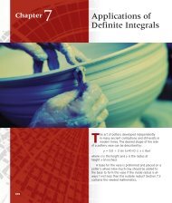
y = 3 cos (2x – p) + 1, y = cos x
(d) The graph has been shifted to the right p2 units. The graph is shown in
Figure 1.45 together with the graph of y cos x. Notice that four periods of
y 3 cos (2x p) 1 are drawn in this window. Now try Exercise 13.
Musical notes are pressure waves in the air. The wave behavior can be modeled with
great accuracy by general sine curves. Devices called Calculator Based Laboratory (CBL)
systems can record these waves with the aid of a microphone. The data in Table 1.18 give
pressure displacement versus time in seconds of a musical note produced by a tuning fork
and recorded with a CBL system.
[–2p, 2p] by [–4, 6]
Figure 1.45 The graph of
y 3 cos(2x p) 1 (blue) and the
graph of y cos x (red). (Example 4)
Table 1.18
Tuning Fork Data
Time Pressure Time Pressure Time Pressure
0.00091 0.080 0.00271 0.141 0.00453 0.749
0.00108 0.200 0.00289 0.309 0.00471 0.581
0.00125 0.480 0.00307 0.348 0.00489 0.346
0.00144 0.693 0.00325 0.248 0.00507 0.077
0.00162 0.816 0.00344 0.041 0.00525 0.164
0.00180 0.844 0.00362 0.217 0.00543 0.320
0.00198 0.771 0.00379 0.480 0.00562 0.354
0.00216 0.603 0.00398 0.681 0.00579 0.248
0.00234 0.368 0.00416 0.810 0.00598 0.035
0.00253 0.099 0.00435 0.827
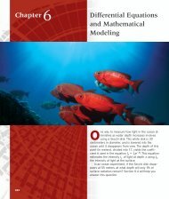
y = 0.6 sin (2488.6x – 2.832) + 0.266
[0, 0.0062] by [–0.5, 1]
Figure 1.46 A sinusoidal regression
model for the tuning fork data in Table 1.18.
(Example 5)
EXAMPLE 5 Finding the Frequency of a Musical Note
Consider the tuning fork data in Table 1.18.
(a) Find a sinusoidal regression equation (general sine curve) for the data and superimpose
its graph on a scatter plot of the data.
(b) The frequency of a musical note, or wave, is measured in cycles per second, or
hertz (1 Hz 1 cycle per second). The frequency is the reciprocal of the period
of the wave, which is measured in seconds per cycle. Estimate the frequency of
the note produced by the tuning fork.
SOLUTION
(a) The sinusoidal regression equation produced by our calculator is approximately
y 0.6 sin (2488.6x 2.832) 0.266.
Figure 1.46 shows its graph together with a scatter plot of the tuning fork data.
2p
(b) The period is sec, so the frequency is 24 88.6
396 Hz.
24 88.6
2p
Interpretation The tuning fork is vibrating at a frequency of about 396 Hz. On the
pure tone scale, this is the note G above middle C. It is a few cycles per second different
from the frequency of the G we hear on a piano’s tempered scale, 392 Hz.
Now try Exercise 23.
Inverse Trigonometric Functions
None of the six basic trigonometric functions graphed in Figure 1.42 is one-to-one. These
functions do not have inverses. However, in each case the domain can be restricted to produce
a new function that does have an inverse, as illustrated in Example 6.