Textbook Chapter 1

You also want an ePaper? Increase the reach of your titles
YUMPU automatically turns print PDFs into web optimized ePapers that Google loves.
46 <strong>Chapter</strong> 1 Prerequisites for Calculus<br />
1.6<br />
What you’ll learn about<br />
•Radian Measure<br />
•Graphs of Trigonometric<br />
Functions<br />
•Periodicity<br />
•Even and Odd Trigonometric<br />
Functions<br />
•Transformations of<br />
Trigonometric Graphs<br />
•Inverse Trigonometric<br />
Functions<br />
. . . and why<br />
Trigonometric functions can be<br />
used to model periodic behavior<br />
and applications such as musical<br />
notes.<br />
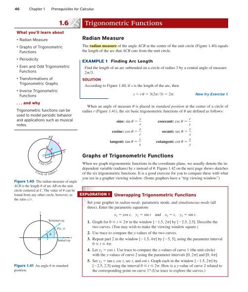
O<br />
y<br />
Terminal ray<br />
r<br />
θ<br />
x<br />
P(x, y)<br />
y<br />
x<br />
Initial ray<br />
Figure 1.41 An angle u in standard<br />
position.<br />
C<br />
Unit<br />
Circle<br />
B<br />
of<br />
B'<br />
1<br />
θ<br />
circle<br />
A<br />
r<br />
radius<br />
Figure 1.40 The radian measure of angle<br />
ACB is the length u of arc AB on the unit<br />
circle centered at C. The value of u can be<br />
found from any other circle, however, as<br />
the ratio sr.<br />
r<br />
s<br />
A'<br />
Trigonometric Functions<br />
Radian Measure<br />
The radian measure of the angle ACB at the center of the unit circle (Figure 1.40) equals<br />
the length of the arc that ACB cuts from the unit circle.<br />
EXAMPLE 1<br />
Finding Arc Length<br />
Find the length of an arc subtended on a circle of radius 3 by a central angle of measure<br />
2p3.<br />
SOLUTION<br />
According to Figure 1.40, if s is the length of the arc, then<br />
s r u 3(2p3) 2p. Now try Exercise 1.<br />
When an angle of measure u is placed in standard position at the center of a circle of<br />
radius r (Figure 1.41), the six basic trigonometric functions of u are defined as follows:<br />
sine: sin u y r <br />
cosine: cos u x r <br />
tangent: tan u y x <br />
Graphs of Trigonometric Functions<br />
cosecant: csc u r <br />
y<br />
secant: sec u r <br />
x<br />
cotangent: cot u x y <br />
When we graph trigonometric functions in the coordinate plane, we usually denote the independent<br />
variable (radians) by x instead of u. Figure 1.42 on the next page shows sketches<br />
of the six trigonometric functions. It is a good exercise for you to compare these with what<br />
you see in a grapher viewing window. (Some graphers have a “trig viewing window.”)<br />
EXPLORATION 1<br />
Unwrapping Trigonometric Functions<br />
Set your grapher in radian mode, parametric mode, and simultaneous mode (all<br />
three). Enter the parametric equations<br />
x 1 cos t, y 1 sin t and x 2 t, y 2 sin t.<br />
1. Graph for 0 t 2p in the window [1.5, 2p] by [2.5, 2.5]. Describe the<br />
two curves. (You may wish to make the viewing window square.)<br />
2. Use trace to compare the y-values of the two curves.<br />
3. Repeat part 2 in the window [1.5, 4p] by [5, 5], using the parameter interval<br />
0 t 4p.<br />
4. Let y 2 cos t. Use trace to compare the x-values of curve 1 (the unit circle)<br />
with the y-values of curve 2 using the parameter intervals [0, 2p] and [0, 4p].<br />
5. Set y 2 tan t, csc t, sec t, and cot t. Graph each in the window [1.5, 2p] by<br />
[2.5, 2.5] using the interval 0 t 2p. How is a y-value of curve 2 related to<br />
the corresponding point on curve 1? (Use trace to explore the curves.)