Textbook Chapter 1

Section 1.3 Exponential Functions 25
1
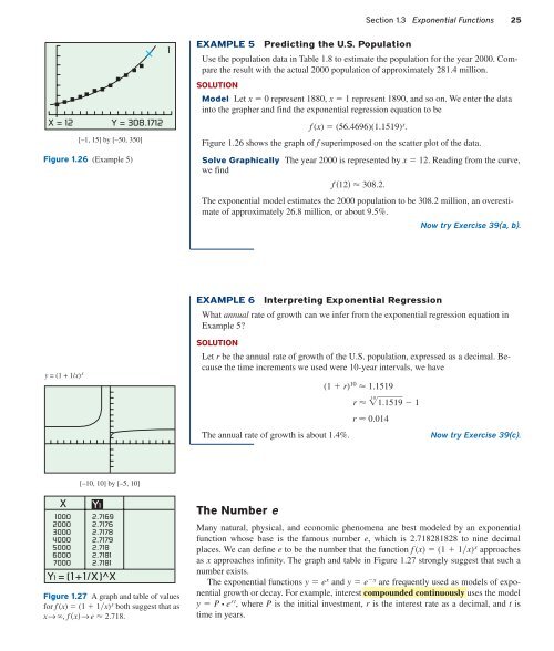
EXAMPLE 5
Predicting the U.S. Population
Use the population data in Table 1.8 to estimate the population for the year 2000. Compare
the result with the actual 2000 population of approximately 281.4 million.
X = 12
Y = 308.1712
[–1, 15] by [–50, 350]
SOLUTION
Model Let x 0 represent 1880, x 1 represent 1890, and so on. We enter the data
into the grapher and find the exponential regression equation to be
f (x) (56.4696)(1.1519) x .
Figure 1.26 shows the graph of f superimposed on the scatter plot of the data.
Figure 1.26 (Example 5)
Solve Graphically The year 2000 is represented by x 12. Reading from the curve,
we find
f 12308.2.
The exponential model estimates the 2000 population to be 308.2 million, an overestimate
of approximately 26.8 million, or about 9.5%.
Now try Exercise 39(a, b).
EXAMPLE 6
Interpreting Exponential Regression
What annual rate of growth can we infer from the exponential regression equation in
Example 5?
y = (1 + 1/x) x
SOLUTION
Let r be the annual rate of growth of the U.S. population, expressed as a decimal. Because
the time increments we used were 10-year intervals, we have
(1 r) 10 1.1519
r 10 1.1519 1
r 0.014
The annual rate of growth is about 1.4%.
Now try Exercise 39(c).
[–10, 10] by [–5, 10]
X
1000
2000
3000
4000
5000
6000
7000
Y1
2.7169
2.7176
2.7178
2.7179
2.718
2.7181
2.7181
Y1 = (1+1/X)^X
Figure 1.27 A graph and table of values
for f (x) (1 1x) x both suggest that as
x→ , f x→ e 2.718.
The Number e
Many natural, physical, and economic phenomena are best modeled by an exponential
function whose base is the famous number e, which is 2.718281828 to nine decimal
places. We can define e to be the number that the function f (x) (1 1x) x approaches
as x approaches infinity. The graph and table in Figure 1.27 strongly suggest that such a
number exists.
The exponential functions y e x and y e x are frequently used as models of exponential
growth or decay. For example, interest compounded continuously uses the model
y P • e rt , where P is the initial investment, r is the interest rate as a decimal, and t is
time in years.