

Journal of Software - Academy Publisher
Journal of Software - Academy Publisher
Journal of Software - Academy Publisher

You also want an ePaper? Increase the reach of your titles
YUMPU automatically turns print PDFs into web optimized ePapers that Google loves.
JOURNAL OF SOFTWARE, VOL. 6, NO. 5, MAY 2011 811<br />
Work out the corresponding eigenvector <strong>of</strong> maximum<br />
eigenvalue <strong>of</strong> B , X = ( x1,<br />
x3,<br />
L,<br />
xn)<br />
, let x i to be the<br />
weight <strong>of</strong> factor u i , then we can get unitary weights<br />
denote W i .<br />
n n<br />
n<br />
A = ( W1,<br />
W2,<br />
L,<br />
Wn)<br />
= ( x1 / ∑ xi<br />
, x2<br />
/ ∑xi, L , xn<br />
/ ∑xi,<br />
)<br />
i=<br />
1 i=<br />
1 i=<br />
1<br />
3) Test <strong>of</strong> Consistency: Because <strong>of</strong> complexity <strong>of</strong><br />
evaluation and limit <strong>of</strong> individual knowledge, the<br />
individual identify matrix may not be consistent with the<br />
actual one, or the disagreement <strong>of</strong> any two identify<br />
matrixes may result in error <strong>of</strong> subjective judgment.<br />
However, we must test the consistency <strong>of</strong> the matrix B as<br />
follows:<br />
① Computing consistency value C ⋅ I<br />
λmax<br />
− n<br />
C ⋅ I =<br />
(31)<br />
n − 1<br />
② Computing consistency ratio C ⋅ R<br />
C ⋅ I<br />
C ⋅ R =<br />
(32)<br />
R ⋅ I<br />
Where R ⋅ I is mean consistency value that can be found<br />
in the reference and forms, we <strong>of</strong>ten consider that if C ⋅ R<br />
is smaller than 0.1, the consistency <strong>of</strong> matrix is<br />
acceptable, otherwise we must modify the identify matrix<br />
B.<br />
4) Computing the General Weight Order: The general<br />
weight order means that the weight order comparing the<br />
elements in the present layer and the highest layer. We<br />
have got each order <strong>of</strong> element in rule layer to the object<br />
layer and the values are W 1, W2<br />
, L , Wn<br />
, respectively, we<br />
also know that order that design layer to the rule layer<br />
j j j<br />
and the values are W W , , W<br />
j ⎛W<br />
⎜ 1<br />
j<br />
j ⎜W2<br />
V = W W = ⎜<br />
⎜ M<br />
⎜ j<br />
⎝Wn<br />
1 , 2 L n , then the general order is<br />
W<br />
W<br />
W<br />
j<br />
1<br />
j<br />
2<br />
M<br />
j<br />
n<br />
j<br />
L W ⎞⎛W<br />
⎞ ⎛V<br />
1 1 1 ⎞<br />
⎟⎜<br />
⎟ ⎜ ⎟<br />
j<br />
L W ⎟⎜W<br />
⎟ ⎜V<br />
2 2 2 ⎟<br />
⎟⎜<br />
⎟ = ⎜ ⎟<br />
M M ⎟⎜<br />
M<br />
⎟ ⎜<br />
M<br />
⎟<br />
j<br />
L W ⎟⎜<br />
⎟ ⎜ ⎟<br />
n ⎠⎝Wn<br />
⎠ ⎝Vn<br />
⎠<br />
, (33)<br />
C. Evaluating the danger level<br />
The entire network <strong>of</strong> danger level should fully reflect<br />
the value <strong>of</strong> each <strong>of</strong> the host facing attacks. As the host <strong>of</strong><br />
each position is not the same such as running a different<br />
system for different users and providing different services,<br />
influencing different economic, affecting different social<br />
and even political values, they are in possession <strong>of</strong><br />
different essentiality.<br />
Let nij (t)<br />
be the numbers <strong>of</strong> i th computers detect<br />
attacking at time t. Let β i ( 0 ≤ βi<br />
≤1)<br />
be the importance<br />
coefficient <strong>of</strong> ith computer in the network and α j<br />
( 0 ≤ α j ≤ 1)<br />
be the danger coefficient <strong>of</strong> the j th kind <strong>of</strong><br />
attack in the network. Then, we can define the attack<br />
intensity ri (t)<br />
<strong>of</strong> the j th kind <strong>of</strong> attack and the<br />
corresponding network danger ri (t)<br />
as follows:<br />
2<br />
ri<br />
( t)<br />
=<br />
− 1<br />
(34)<br />
1 + e<br />
© 2011 ACADEMY PUBLISHER<br />
−<br />
∑<br />
α jnij<br />
j<br />
8<br />
Let Importancei<br />
= ∑ ( I k × Wk<br />
) be the importance<br />
k=<br />
1<br />
coefficient <strong>of</strong> j th host in the network. Then, we obtain the<br />
network entire danger level value: R(t) =∑(indicator<br />
value × indicator weight). Therefore, we can get network<br />
danger R(t) situation and evaluate network security at real<br />
time.<br />
N n<br />
R(<br />
t)<br />
= tanh( ∑(<br />
∑(<br />
Hosti<br />
's<br />
danger×<br />
Importancej<br />
) × LCRS_Weightm<br />
))<br />
m=<br />
1 i=<br />
1<br />
N n<br />
8<br />
= tanh( ∑(<br />
∑( Hosti<br />
's<br />
danger×<br />
∑(<br />
I j,<br />
k × Wk<br />
) ) × LCRS_Weightm<br />
))<br />
m=<br />
1 i= 1<br />
k=<br />
1<br />
N n 8<br />
= tanh( ∑(<br />
∑( ri<br />
( t)<br />
× ∑(<br />
I j,<br />
k × Wk<br />
)) × LCRS_Weightm<br />
))<br />
m=<br />
1 i= 1 k=<br />
1<br />
(35)<br />
The conclusion can be shown that the higher value R(t)<br />
reaches the more dangerous the network is.<br />
Ⅴ.EXPERIMENTAL RESULTS AND ANALYSIS<br />
A. Experimental Environment and Evaluation Indicators<br />
Experiments <strong>of</strong> attack simulation were also carried<br />
out in our Laboratory. Analytic Hierarchy Process is<br />
applied to our model to evaluate the weights <strong>of</strong> the<br />
indicators in the experiments. Considering the preciseness<br />
and efficiency, we use 12 indicators to evaluate the<br />
network danger, which include host danger, area danger,<br />
cells danger, special danger etc. The weights <strong>of</strong> the<br />
indicators are evaluated and sorted by orders and the<br />
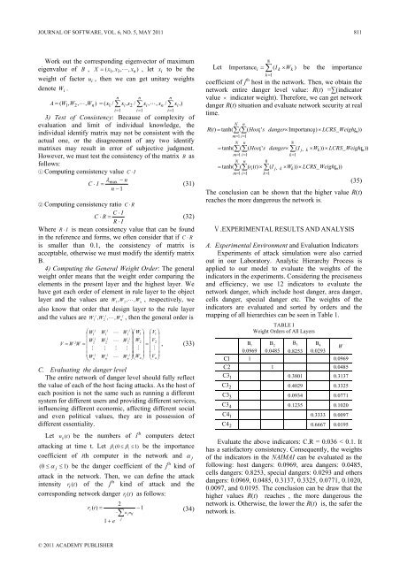
mapping <strong>of</strong> all hierarchies can be seen in Table 1.<br />
B 1<br />
0.0969<br />
TABLE I<br />
Weight Orders <strong>of</strong> All Layers<br />
B 2<br />
0.0485<br />
B 3<br />
0.8253<br />
B 4<br />
0.0293<br />
C 1 1 0.0969<br />
C 2<br />
1 0.0485<br />
C 31<br />
0.3801 0.3137<br />
C 32<br />
0.4029 0.3325<br />
C3 3<br />
0.0934 0.0771<br />
C3 4<br />
0.1235 0.1020<br />
C 41<br />
0.3333 0.0097<br />
C 42<br />
0.6667 0.0195<br />
Evaluate the above indicators: C.R = 0.036 < 0.1. It<br />
has a satisfactory consistency. Consequently, the weights<br />
<strong>of</strong> the indicators in the NAIMAI can be evaluated as the<br />
following: host dangers: 0.0969, area dangers: 0.0485,<br />
cells dangers: 0.8253, special dangers: 0.0293 and others<br />
dangers: 0.0969, 0.0485, 0.3137, 0.3325, 0.0771, 0.1020,<br />
0.0097, and 0.0195. The conclusion can be draw that the<br />
higher values R(t) reaches , the more dangerous the<br />
network is. Otherwise, the lower the R(t) is, the safer the<br />
network is.<br />
W


