Journal of Software - Academy Publisher

942 JOURNAL OF SOFTWARE, VOL. 6, NO. 5, MAY 2011
linear structure in the system model that can be even
extracted from the system model and use Kalman filter
for solving, such as Rao-Blackwellize method [13]. So
when using particle filter, such component with simple
structure can be easily estimated. For horizontal map
errors, the convergence of Y direction is worse than the X
direction, that because the terrain in the second half path
varies more on the X direction than Y direction which
benefits the component estimation on X direction.
Meanwhile, the convergent speed for horizontal errors is
very slow which may caused by the constant
characteristic of these states.
220
200
180
Horizontal X direction
0 50 100 150 200 250 300
Horizontal Y direction
200
150
100
0 50 100 150
Vertical
200 250 300
200
100
0
0 50 100 150 200 250 300
Figure 6. Map error estimation.
Fig. 7 and Fig. 8 show the particle evolution process
for SIS and RPF respectively for comparison of the
effectiveness of these two different algorithms. The
figures show the histogram of one component of the state
in the particle set at different time step which can be seen
as the distribution of that component. The component we
chose to show is the X direction error of the map error
component which is a constant parameter in the state
vector.
Fig. 7 is for SIS. As mentioned above, the commonly
used particle filter is not suitable for solving the model
with constant parameters. For these parameters the initial
particle set at k=1 contains the whole data values for the
evolution that there will be no new values generated in
later time step since they have no process noise. So the
initial distribution must cover the true value we estimated
otherwise the filter can not give that value. From Fig. 7,
after several iterations the distribution is concentrated to
some distinct values and the state can hardly move to
other values.
In Fig. 7, when k=1, the initial distribute is a Gaussian
distribution with mean equal to 180 and can cover the
true value of 200 which is the map error we set. After
some iterations, the amount of effective values decreases
and when k=16 there are only two bars in the histogram
which do not contain the true value thus after that the
filter can not give the accurate value of 200.
In SIS, since the parameter components in the particle
do not change during state transition step, the degeneracy
phenomenon of these components will affect the
evolution of the other state components and lead to slow
© 2011 ACADEMY PUBLISHER
convergent speed, low accuracy and even divergent when
the particles fall into bad bars.
x 104
k=1
4
2
0
80 100 120 140 160 180 200 220 240 260 280
x 104
k=6
4
2
0
80 100 120 140 160 180 200 220 240 260 280
x 104
k=9
4
2
0
80 100 120 140 160 180 200 220 240 260 280
x 104
k=16
4
2
0
80 100 120 140 160 180 200 220 240 260 280
Figure 7. particle evolution for SIS.
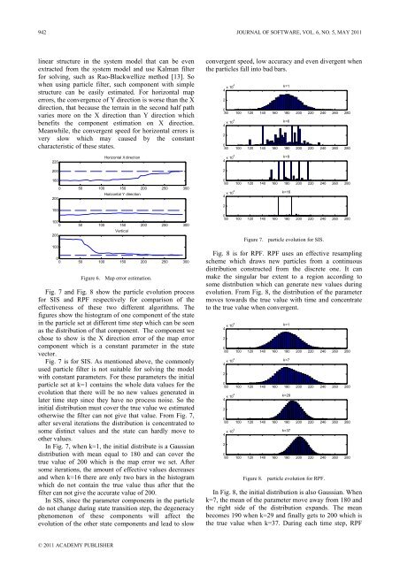
Fig. 8 is for RPF. RPF uses an effective resampling
scheme which draws new particles from a continuous
distribution constructed from the discrete one. It can
make the singular bar extent to a region according to
some distribution which can generate new values during
evolution. From Fig. 8, the distribution of the parameter
moves towards the true value with time and concentrate
to the true value when convergent.
x 104
k=1
4
2
0
80 100 120 140 160 180 200 220 240 260 280
x 104
k=7
4
2
0
80 100 120 140 160 180 200 220 240 260 280
x 104
k=29
4
2
0
80 100 120 140 160 180 200 220 240 260 280
x 104
k=37
4
2
0
80 100 120 140 160 180 200 220 240 260 280
Figure 8. particle evolution for RPF.
In Fig. 8, the initial distribution is also Gaussian. When
k=7, the mean of the parameter move away from 180 and
the right side of the distribution expands. The mean
becomes 190 when k=29 and finally gets to 200 which is
the true value when k=37. During each time step, RPF