Contents - Industrial and Operations Engineering

Contents
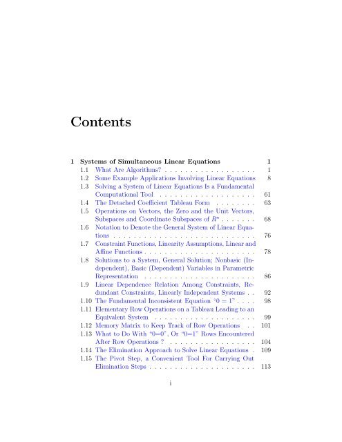
1 Systems of Simultaneous Linear Equations 1
1.1 What Are Algorithms? . . . . . . . . .. . . . . . . . . 1
1.2 Some Example Applications Involving Linear Equations 8
1.3 Solving aSystem of Linear Equations Is aFundamental
Computational Tool . . . . . . . . . .. . . . . . . . . 61
1.4 The Detached Coefficient Tableau Form . . . . . . . . 63
1.5 Operations on Vectors, the Zero and the Unit Vectors,
Subspaces and Coordinate Subspaces of R n . . . . . . . 68
1.6 Notation to Denote the General System of Linear Equations
. . . . . . . .. . . . . . . . . . .. . . . . . . . . 76
1.7 ConstraintFunctions, LinearityAssumptions, Linearand
Affine Functions . .. . . . . . . . . . .. . . . . . . . . 78
1.8 Solutions to aSystem, General Solution; Nonbasic (Independent),
Basic (Dependent) Variables in Parametric
Representation . .. . . . . . . . . . .. . . . . . . . . 86
1.9 Linear Dependence Relation Among Constraints, Redundant
Constraints, Linearly Independent Systems . . 92
1.10 The Fundamental Inconsistent Equation “0 =1”. . . . 98
1.11 Elementary Row Operations on aTableau Leading to an
Equivalent System . . . . . . . . . . .. . . . . . . . . 99
1.12 Memory Matrix to Keep Track of Row Operations . . 101
1.13 What to Do With “0=0”, Or “0=1” Rows Encountered
After Row Operations ? . . . . . . . .. . . . . . . . . 104
1.14 The Elimination Approach to Solve Linear Equations . 109
1.15 The Pivot Step, aConvenient Tool For Carrying Out
Elimination Steps .. . . . . . . . . . .. . . . . . . . . 113
i

ii
1.16 The Gauss-Jordan(GJ) Pivotal Method for Solving Linear
Equations . . .. . . . . . . . . . .. . . . . . . . . 120
1.17 ATheorem of Alternatives for Systems of Linear Equations
. . . . . . . .. . . . . . . . . . .. . . . . . . . . 145
1.18 Special Triangular Systems of Linear Equations . . . . 149
1.19 The Gaussian Pivot Step . . . . . . . .. . . . . . . . . 154
1.20 The Gaussian (G) Elimination Method for Solving Linear
Equations . . .. . . . . . . . . . .. . . . . . . . . 157
1.21 Comparison of the GJ and the GElimination Methods 165
1.22 Infeasibility Analysis . . . . . . . . . .. . . . . . . . . 165
1.23 Homogeneous Systems of Linear Equations . . . . . . . 171
1.24 Solving Systems of Linear Equations And/Or Inequalities177
1.25 Can WeObtain aNonnegative Solution to aSystem of
Linear Equations by the GJ or the GMethods Directly? 178
1.26 Additional Exercises . . . . . . . . . .. . . . . . . . . 178
1.27 References . . . . .. . . . . . . . . . .. . . . . . . . . 183

Chapter 1
Systems of Simultaneous
Linear Equations
This is Chapter 1 of “Sophomore Level Self-Teaching Webbook
for Computational and Algorithmic Linear Algebra and
n-Dimensional Geometry” by Katta G. Murty.
1.1 What Are Algorithms?
Algorithms are procedures for solving computational problems. Sometimes
algorithms are also called methods.
An algorithm for a computational problem is a systematic stepby-step
procedure for solving it that is so clearly stated without any
ambiguities that it can be programmed for execution by a machine (a
computer).
Historical note on algorithms: The word “algorithm” originated
from the title of the Latin translation of a book
Algoritmi de Numero Indorum
meaning Al-Khwarizmi Concerning the Hindu Art of Reckoning. Itwas
written in 825 AD by the Arabic scholar “Muhammad Ibn Musa Al-
Khwarizmi” who lived in Iraq, Iran (mostly Baghdad); and was based—
1

2 Ch.1.Lineareqs.
on earlier Indian and Arabic treatizes. This book survives only in its
Latin translation, as all the copies of the original Arabic version have
been lost or destroyed.
Algorithms seem to have originated in the work of ancient Indian
mathematicians on rules for solving linear and quadratic equations.
As an illustrative example, we provide the following problem and
discuss an algorithm for solving it:
Problem 1: Input: Given positive integer n. Required output:
Find all prime numbers ≤ n.
A prime number is a positive integer > 1 that is divisible only by
itself and by 1.
We provide an algorithm for this problem dating back to the 3rd
century BC, known as the Eratosthenes Sieve.
Algorithm: Eratosthenes Sieve for Finding All Prime Numbers
≤ n
BEGIN
Initial Step: Write all integers 1 to n in increasing order from left
to right. Strike off 1 and put a pointer at 2, the first prime.
General Step: Suppose pointer is now on r. Counting from r,
strike off every rth number to the right.
If all numbers to the right of r are now struck off, collect all the
numbers in the list that are not struck off. These are all the primes
≤ n, terminate.
Otherwise move the pointer right to the next number not struck
off, and repeat this general step with the pointer in its new position.
END
Example 1: Illustration of Eratosthenes Sieve f or
n = 10

1.1. Algorithms 3
We will now apply this algorithm on the instance of the problem
with n = 10. At the end of Step 1, the sequence of numbers written
looks like this:
� 1, 2
, 3, 4, 5, 6, 7, 8, 9, 10
↑
After the General step is applied once, the sequence of numbers
looks like this:
� 1, 2, 3
, � 4, 5, � 6, 7, � 8, 9, � 10
↑
Applying the General step again, we get this:
� 1, 2, 3, � 4, 5
, � 6, 7, � 8, � 9, � 10
↑
Applying the General step again, we get this:
� 1, 2, 3, � 4, 5, � 6, 7
, � 8, � 9, � 10
↑
Now all the numbers to the right of the pointer are struck off, so
we can terminate. The set of numbers not struck off is {2, 3, 5, 7},
this is the set of all primes ≤ 10. ⊲⊳ 1
There may be several different algorithms for solving a problem.
The mathematical characterization of the most efficient algorithm for a
problem is quite complicated. Informally, we will say that an algorithm
for solving a problem is more efficient than another if it is faster or
requires less computational effort.
It usually requires a deep study of a problem to uncover details of
its structure and find good characterizations of its solution, in order
to develop efficient algorithms for it. We will illustrate this statement
with an example of a problem in networks and an efficient algorithm
for it that came out of a deep study of the problem.
A network consists of points called nodes, andedges each of
which is a line joining a pair of nodes. Such networks are used to
model and represent the system of streets in a city, in transportation,
1 This symbol indicates the end of this portion of text, here Example 1.

4 Ch.1.Lineareqs.
1 2
4
5
3
Figure 1.1:
routing, traffic flow, and distribution studies. In this representation
street intersections or traffic centers are represented by nodes in the
network and two-way street segments joining adjacent intersections are
represented by edges.
A network is said to be connected if it is possible to travel from
any node to any other node in the network using only the edges in
the network. Figure 1.1 is a network in which nodes are numbered
and drawn as little circles, and each edge joins a pair of nodes. This
network is clearly connected.
An Euler circuit (named after the 18th century Swiss Mathematician
Leonhard Euler) in a connected network is a route which begins at
a node, say node 1, goes through each edge of the network exactly once,
and returns to the starting node, node 1, at the end. Euler circuits play
an important role in problems such as those of finding least distance
routes for postmen’s beats, good routes for school buses and garbage
collection vehicles, etc.
As an example, in the network with 5 nodes and 7 edges in Figure
1.2, traveling along the edges in the order and direction indicated in

1.1. Algorithms 5
Figure 1.2 (the edge joining nodes 1 and 2 is traveled first in the directionfrom1to2,thentheedgejoiningnodes2and3fromnode2to
node 3, etc.) leads to one Euler circuit in this network.
Now we describe the problem.
Problem 2: Given a connected network G with nodes 1,...,n,
check whether there is an Euler circuit in it.
Notice that Problem 2 only poses the question of the existence of
an Euler circuit, it does not ask for an Euler circuit when one exists.
Someone who has read Problem 2 for the first time may try to
develop an algorithm for it by beginning at node 1, and then tracing
the edges in some order without repeating any edge in an effort to
construct an Euler circuit. But the most efficient algorithm for it is
an indirect algorithm developed by L. Euler in the year 1736. The
algorithm described below, only answers the existence question, and
does not output an Euler circuit.
5
4
7
4
1
6
3
5
1
3
2
2
Figure 1.2:

6 Ch.1.Lineareqs.
Euler’s algorithm for Problem 2
BEGIN
Define the degree of a node in G to be the number of edges containing
it. Find the degree of each node in G.
If the degree of every node in G is an even number, there is an Euler
circuit in G. IfatleastonenodeinG has odd degree, there is no Euler
circuit in G. Terminate.
END
Example 2: Illustration of Euler’s Algorithm to
check t he ex is tence o f a n Euler circuit
Let di denote the degree of node i. For the network in Figure 1.2,
we have (d1,d2,d3,d4,d5) =(2, 4, 2, 2, 4). Since all these node degrees
are even, this network has an Euler circuit. An Euler circuit in it was
given above.
For the network in Figure 1.1, we have (d1,d2,d3,d4,d5) =(5, 5, 5, 5, 4).
Since there are some odd numbers among these node degrees, this network
has no Euler circuit by the above algorithm.
The basis for this algorithm is a very beautiful theorem proved by
L. Euler in the year 1736 that a connected network has an Euler circuit
iff the degree of every node in it is even.
The branch of science dealing with the development of efficient algorithms
for a variety of computational problems is the most challenging
area of research today.
Exercises
1.1.1: Apply the Eratostenes Sieve to find all prime numbers ≤
n = 22.

1.1. Algorithms 7
5
10
4
9
1
6
8
Figure 1.3: Network for Exercise 1.1.2
1.1.2: Consider the network in Figure 1.3. Check whether this network
has an Euler circuit using the algorithm discussed above. Verify
the correctness of the answer by actually trying to construct an Euler
circuit beginning with node 1 and explain your conclusion carefully.
⊲⊳
In this book we will discuss algorithms for solving systems of linear
equations, and other related linear algebra problems.
Systems of simultaneous linear equations pervade all technical areas.
Knowledge about models involving simultaneous linear equations,
and the fundamental concepts behind algorithms for solving and analyzing
them, is extremely important for everyone with aspirations of
getting any technical job. Also, systems of simultaneous linear equations
lie at the heart of computational methods for solving most mathematical
models, as many of these methods include steps that require
the solution of such systems. Hence the material discussed in this chapter
is very fundamental, and extremely important for all students of
engineering and the applied sciences.
7
3
2

8 Ch.1.Lineareqs.
We begin with some example applications that lead to models involving
simultaneous linear equations.
1.2 Some Example Applications Involving
Linear Equations
Example 1: Scrap Metal Blending Problem
Consider the following problem. A steel company has four different
types of scrap metal (called SM-1 to SM-4) with the following compositions:
Type % in type, by weight, of element
Al Si C Fe
SM-1 5 3 4 88
SM-2 7 6 5 82
SM-3 2 1 3 94
SM-4 1 2 1 96
They need to blend these four scrap metals into a mixture for which
the composition by weight is:
Al - 4.43%, Si - 3.22%, C - 3.89%, Fe - 88.46%.
How should they prepare this mixture ? To answer this question,
we need to determine the proportions of the 4 scrap meatals SM-1,
SM-2, SM-3, SM-4 in the blend to be prepared.
Historical note on algebra, linear algebra: The most fundamental
idea in linear algebra which was discovered more than 5000
years ago by the Chinese, Indians, Iranians, and Babylonians, is to
represent the quantities that we like to determine by symbols; usually
letters of the alphabet like x, y, z; and then express the relationships
between the quantities represented by these symbols in the form of—

1.2 Example applications 9
equations, and finally use these equations as tools to find out the true
values represented by the symbols. The symbols representing the unknown
quantities to be determined are nowadays called unknowns or
variables or decision variables.
The process of representing the relationships between the variables
through equations or other functional relationships is called modeling
or mathematical modeling.
Linear algebra gradually evolved into algebra, one of the chief branches
of mathematics. Even though the subject originated more than 5000
years ago, the name algebra itself came much later, it is derived from
the title of an Arabic book Hisab al-jabr w’almuqabalah written by the
same mathematician Al-Khowarizmi discussed in Section 1.1, around
the same year 825 AD. The term “al-jabr” in Arabic means “restoring”
in the sense of solving an equation. In Latin translation the title of this
book became Ludus Algebrae, the second word in this title surviving
as the modern word algebra for the subject.
The word linear in “linear angebra” refers to the “linear combinations”
(see Sections 1.5, 3.5) in the spaces studied, and the linearity of
“linear functions” (see Section 1.7) and “linear equations” studied in
the subject.
Model for scrap metal blending problem: Returning to our
scrap metal blending problem, in order to model it, we first define the
decision variables, denoted by x1,x2,x3,x4, whereforj =1to4
xj = proportion of SM-j by weight in the mixture
Then the percentage by weight, of the element Al in the mixture
will be, 5x1 +7x2 +2x3 + x4, which is required to be 4.43. Arguing
the same way for the elements Si, C, and Fe, we find that the decision
variables x1 to x4 must satisfy each equation in the following system
of linear equations in order to lead to the desired mixture:
5x1 +7x2 +2x3 + x4 = 4.43
3x1 +6x2 + x3 +2x4 = 3.22

10 Ch.1.Lineareqs.
4x1 +5x2 +3x3 + x4 = 3.89
88x1 +82x2 +94x3 +96x4 = 88.46
x1 + x2 + x3 + x4 = 1
The last equation in the system stems from the fact that the sum of
the proportions of various ingradients in a blend must always be equal
to 1. This system of equations is the mathematical model for our scrap
metal blending problem. By solving it, we will find the values of the
decision variables x1 to x4 that define the desired blend.
Discussion
RHS Constants, Coefficients
It is customary to write the equations as above with the terms
involving the variables on the left hand side (LHS) of the “=”
sign, and the constant terms on the right hand side (RHS). The
constant term appearing on the RHS of each equation is known as
the RHS constant in that equation. The RHS constant in the first
equation is 4.43, etc.
The number “5” appearing on the LHS of the first equation in
the system is known as the coefficient of the variable x1 in that
equation, etc.
In this system of equations, every variable appears with a nonzero
coefficient in every equation. If a variable does not appear in an equation,
we will say that its coefficient in that equation is zero, and vice
versa.
A variable is considered to be in the system iff it has a nonzero
coefficient in at least one of the constraints. Therefore, every variable
in the system must have a nonzero coefficient in at least one equation.
Moving Terms from Left to Right &Vice Versa
Terms can be moved from left to right (or vice versa) across the
“=” symbol by multiplying them by a “−” sign. The justification for
this comes from the principle that when you add equal amounts to equal

1.2 Example applications 11
quantities, the resulting quantities will be equal. In other words, when
you add the same quantity to both sides of an equation, the equation
continues to be valid. For example, the first equation in the above
system is:
5x1 +7x2 +2x3 + x4 = 4.43
Suppose we want to move the 7x2 term in this equation from
the left side to the right side of the “=” symbol. Add −7x2 to both
sides of this equation. By the above principle this leads to:
5x1 +7x2 +2x3 + x4 − 7x2 = 4.43 − 7x2
On the left hand side the +7x2 and the −7x2 terms cancel with
each other, leading to:
5x1 +2x3 + x4 = 4.43 − 7x2
Notice that the sign of this term has changed as it moved from
the left to the right of the equality symbol in this equation. In the
same way, we can write the first constraint in an equivalent manner by
moving the constant term from the right side of “=” to the left side
as:
5x1 +7x2 +2x3 + x4 − 4.43 = 0
Another equivalent way of writing the first constraint is:
5x1 = 4.43 − 7x2 − 2x3 − x4
Nonnegativity Restrictions on the Variables
The system in this example consists of 5 equations in 4 variables.
From the definition of the variables given above, it is clear that a solution
to this system of equations makes sense for the blending application
under consideration, only if all the variables in the system have
nonnegative values in it. Each nonnegative solution to this system of

12 Ch.1.Lineareqs.
equations leads to a desirable mixture. The nonnegativity restrictions
on the variables are linear inequality constraints. They cannot be
expressed in the form of linear equations, and since the focus of this
book is linear equations, for the moment we will ignore them.
System of Equations, Solutions, Vectors
In the system of equations obtained above, each equation is associated
with a specific requirement in the problem. For example, equations
1 to 4 are associated with the requirements of the elements Al,
Si, C, Fe respectively in the mixture; and equation 5 must be satisfied
by any blend, hence, we will call it the blending requirement.
In the same way, each decision variable in the system is associated
with a unique scrap metal that can be included in the blend.
A system like this is called a system of linear equations, ormore
precisely, a system of simultaneous linear equations because a
solution is required to satisfy all the equations in the system.
Using the Gauss-Jordan (GJ) elimination method discussed later
in Section 1.16, it can be determined that this system has the unique
solution:
¯x =(¯x1, ¯x2, ¯x3, ¯x4) =(0.25, 0.34, 0.39, 0.02)
which happens to be also nonnegative. Thus a mixture of desired
composition can only be obtained by mixing the scrap metals in the
following way:
Scrap metal %byweightinblend
SM1 25
SM2 34
SM3 39
SM4 2
The solution ¯x =(¯x1, ¯x2, ¯x3, ¯x4) =(0.25, 0.34, 0.39, 0.02) is called a
solution vector to the system of equations. A solution, or solution
vector for a system of linear equations, gives specific numerical values

1.2 Example applications 13
to each variable in the system that together satisfy all the equations in
the system.
The word vector in this book refers to a set of numbers arranged
in a specified order, that’s why it is called an ordered set of numbers.
It is an ordered set because the first number in the vector is
the proportion by weight of the specific raw material SM1, the second
number is the proportion by weight of SM2, etc. Hence, if we change
the order of numbers in a vector, the vector changes; i.e., for example
(0.25, 0.34, 0.39, 0.02) and (0.34, 0.25, 0.39, 0.02) are not the same
vector.
A vector giving specific numerical values to each variable in a system
of linear equations is said to be a solution or feasible solution for
the system if it satisfies every one of the equations in the system. A
vector violating at least one of the equations in the system is said to
be infeasible to the system.
Since it has four entries, ¯x above is said to be a four dimensional
vector. An n dimensional vector will have n entries.
The definition of vector that we are using here is standard in all
mathematical literature. The word “vector” is also used to represent
a directed line segment joining a pair of points in the two dimensional
plane in geometry and physics. Using the same word for two different
concepts confuses young readers. To avoid confusion, we will use the
word “vector” to denote an ordered set of numbers only in this book.
For the other concept “the direction from one point towards another
point” in space of any dimension we will use the word “direction” itself
or the phrase “direction vector”(see Section 3.5).
As we will learn later, vectors can be of two types, row vectors and
column vectors. If the entries in a vector are written horizontally one
after the other, the vector is called a row vector. The solution vector
¯x is a row vector. If the entries in a vector are written vertically one
below the other, the vector is called a column vector.
The symbol R n denotes the set of all possible n dimensional vectors
(either row vectors or column vectors). If u is an n dimensional vector
with entries u1,...,un in that order, each ui is a real number; and we
indicate this by u ∈ R n (i.e., u is contained in R n ). An n dimensional
vector is also called an n-tuple or an n-tuple vector.

14 Ch.1.Lineareqs.
In the n-dimensional vector x =(x1,...,xj−1,xj,xj+1,...,xn), xj
is known as the j-th entry or j-th component or j-th coordinate
of the vector x, forj =1ton.
R n is called the n-dimensional vector space, orthespace of all
n-dimensional vectors.
Historical note on vectors: The original concept of a vector
(ordered set of numbers, also called a sequence now-a-days) goes back
to prehistoric times in ancient India, in the development of the position
notation for representing numbers by an ordered set or sequence of
digits. There are 10 digits, these are 0, 1, ..., 9. When we write the
number 2357 as a sequence of digits ordered from left to right, we are
using a notation for the number which is actually 7 + 5(10) + 3(10 2 )+
2(10 3 ).
In the symbol “2357” the rightmost digit 7 is said to be in the
“digits position”. The next digit 5 to the left is in the “10s position”.
The next one 3 to the left is in the “100s position”, or “10 2 s position”;
and so on. Clearly changing the order of digits in a number changes
its value, that’s why it is important to treat the digits in a number as
an ordered set or sequence, which we are now calling a vector.
In the number 904 = 4 + 9(10 2 ), there is no entry in the 10s position.
For representing such numbers the people who developed the
position notation in ancient India realized that they had to introduce a
symbol for “nothing” (“sunya” in Sanskrit), and introduced the symbol
“0” (sunna) for zero or “nothing”. It is believed that zero got introduced
officially as a digit through this process, even though it was not
recognized as a number until then.
Ex ample 2 : Athlete’s Supplemental Diet Formulation
The nutritionist advising a promising athlete preparing for an international
competition has determined that his client needs 110 units
of Vitamin E, 250 units of Vitamin K, and 700 calories of stored muscular
energy (SME) per day in addition to the normal nutrition the
client picks up from a regular diet. These additional nutrients can be

1.2 Example applications 15
picked up by including five different supplemental foods with the following
compositions (remember that the units of measurement of each
supplemental food and each nutrient may be different, for example one
may be measured in liters, another in Kg, etc.).
Nutrient Nutrient units/unit of food
Food 1 Food 2 Food 3 Food 4 Food5
Vit E 50 0 80 90 4
Vit K 0 0 200 100 30
SME 100 300 50 250 350
A supplemental diet specifies the quantity of each of foods 1 to 5 to
include in the athlete’s daily intake. In order to express mathematically
the conditions that a supplemental diet has to satisfy to meet all the
requirements, we define the decision variables: for j =1to5
xj = units of food j in the supplemental diet
The total amount of Vit E contained in the supplemental diet represented
by the vector x =(x1,x2,x3,x4,x5) is 50x1+80x3+90x4+4x5
units. Unfortunately, not all of this quantity is absorbed by the body,
only a fraction of it is absorbed and the rest discarded. The fraction
absorbed varies with the food and the nutrient, and is to be determined
by very careful (and tedious) metabolic analysis. This data is
given below.
Nutrient Prop. nutrient absorbed, in food
Food 1 Food 2 Food 3 Food 4 Food 5
Vit E 0.6 − 0.8 0.7 0.9
Vit K − − 0.4 0.6 1.0
SME 0.5 0.6 0.9 0.4 0.8
So the units of Vit E absorbed by the athlete’s body in the supplemental
diet represented by x is 50×0.6x1 +80×0.8x3 +90×0.7x4 +
4 × 0.9x5, which is required to be 110. Arguing the same way with
Vit K, and Calories of SME, we find that the decision variables x1 to

16 Ch.1.Lineareqs.
x5 must satisfy the following system of linear equations in order to
yield a supplemental diet satisfying all the nutritionist’s requirements:
30x1 +64x3 +63x4 +36x5 = 110
80x3 +60x4 +30x5 = 250
50x1 + 180x2 +45x3 + 100x4 + 280x5 = 700
This is a system of three equations in five variables. Of course, here
also, in addition to these equations, the variables have to satisfy the
nonnegativity restrictions, which we ignore.
Example 3: A Coin Assembly Problem
A class in an elementary school was assigned the following project
by their teacher. They are given an unlimited supply of US coins consisting
of: pennies (1 cent), nickels (5 cents), dimes (10 cents), quarters
(25 cents), half dollars (50 cents), and dollars. They are required to
assemble a set of these coins satisfying the following constraints:
Total value of the set has to be equal to $31.58
Total number of coins in the set has to be equal to 171
Total weight of the set has to be equal to 735.762 grams.
Here is the weight data:
Coin Weight in grams
Penny 2.5
Nickel 5.0
Dime 2.268
Quarter 5.67
Half Dollar 11.34
Dollar 8.1
Formulate the class’s problem as a system of linear equations.
Let the index j = 1 to 6 refer to penny, nickel, dime, quarter, half

1.2 Example applications 17
dollar, and dollar, respectively. For j = 1 to 6 define the decision
variable:
xj = number of coins of coin j in the assembly
Then the constraints to be satisfied by the solution vector x =
(x1,x2,x3,x4,x5,x6) corresponding to an assembly satisfying the
teacher’s requirements are:
0.01x1 +0.05x2 +0.10x3 +0.25x4 +0.5x5 + x6 = 31.58
x1 + x2 + x3 + x4 + x5 + x6 = 171
2.5x1 +5.0x2 +2.268x3 +5.67x4 +11.34x5 +8.1x6 = 735.762
Of course, in addition to these equations, we require the variables
to be not only nonnegative, but nonnegative integers; but we ignore
these requirements for the moment.
Example 4 : Balancing chemical reactions
In a chemical reaction, two or more input chemicals combine and react
to form one or more output chemicals. Balancing this chemical
reaction deals with the problem of determining how many molecules
of each input chemical participate in this reaction, and how many
molecules of each output chemical are produced in the reaction. This
leads to a system of linear equations for which the simplest positive
integer solution is needed.
As an example, consider the well known reaction in which molecules
of hydrogen (H) and oxygen (O) combine to produce molecules of water.
A molecule of hydrogen (oxygen) consists of two atoms of hydrogen
(oxygen) and is represented as H2 (O2); in the same way a molecule of
water consists of two atoms of hydrogen and one atom of oxygen and
is represented as H2O. The question that arises about this reaction is:
how many molecules of hydrogen combine with how many molecules of
oxygen in the reaction, and how many molecules of water are produced
as a result. Let

18 Ch.1.Lineareqs.
x1,x2,x3 denote the number of molecules of hydrogen, oxygen,
water respectively, involved in this reaction.
Then this chemical reaction is represented as:
x1H2 + x2O2 −→ x3H2O
Balancing this chemical reaction means finding the simplest positive
integral values for x1,x2,x3 that leads to the same number of atoms of
hydrogen and oxygen, the two elements appearing in this reaction, on
both sides of the arrow.
Equating the atoms of each element on both sides of the arrow leads
to an equation that the variables have to satisfy. In this reaction those
equations are: 2x1 =2x3 for hydrogen atoms, and 2x2 = x3 for oxygen
atoms. This leads to the system of equations:
2x1 − 2x3 = 0
2x2 − x3 = 0
in x1,x2,x3. x1 =2,x2 =1,x3 = 2 leads to a simple integer solution
to this system, leading to the balanced reaction 2H2 + O2 −→ 2H2O.
In the same way balancing any chemical reaction leads to a system
of linear equations in which each variable is associated with either an
input, or an output chemical; and each constraint corresponds to a
chemical element in some of these chemicals. We require the simplest
positive integer solution to this system, but for the moment we will
ignore these requirements.
Example 5: Parameter Estimation in Curve Fitting
Using t he Metho d of Least Squares
A common problem in all areas of scientific research is to obtain
a mathematical functional relationship between a variable, say t, and
avariabley whose value is known to depend on the value of t; from
data on the values of y corresponding to various values of t, usually
determined experimentally. Suppose this data is:

1.2 Example applications 19
when t = tr, theobservedvalueofy is yr; forr =1tok.
Using this data, we are required to come up with a mathematical
expression for y as a function of t. This problem is known as a curve
fitting problem, handling it involves the following steps.
Algorithm for Solving a Curve Fitting Problem
BEGIN
Step 1: Select a model function f(t)
An explicit mathematical function, let us denote it by f(t), containing
possibly several unknown parameters (or numerical constants with
unknown values) that seems to provide a good fit for y is selected in this
step. The selected function is called the model function. Theremay
be theoretical considerations which suggest a good model function. Or
one can create a plot of the observed data on the 2-dimensional Cartesian
plane, and from the pattern of these points think of a good model
function.
Step 2: Parameter estimation
Let a0,a1,...,an denote the parameters in the model function f(t)
whose numerical values are unknown.
Measuring the values of y experimentally is usually subject to unknown
random errors, so even if the model function f(t) isanexact
fit for y, we may not be able to find any values of the parameters
a0,a1,...,an that satisfy:
yr = observed value of y when t = tr is = f(tr), for r =1
to k.
In this step we find the best values for the parameters a0,...,an
that make f(tr) asclosetoyr as possible, for r =1tok.
The method of least squares for parameter estimation selects the
values of the parameters a0,...,an in f(t) to be those that minimize
the sum of squares of deviations (yr −f(tr)) over r=1to k; i.e.,——

20 Ch.1.Lineareqs.
k�
minimize L2(a0,...,an) = (yr − f(tr))
r=1
2
The vector (ā0,...,ān) that minimizes L2(a0,...,an) isknownas
the least squares estimator for the parameter vector; and with the
values of the parameters (a0,...,an) fixedat(ā0,...,ān), the function
f(t) isknownastheleast squares fit for y as a function of t.
From calculus we know that a necessary condition for (ā0,...,ān)to
minimize L2(a0,...,an) isthatitmustsatisfytheequationsobtained
by setting the partial derivatives of L2(a0,...,an) WRT a0,...,an
equal to 0.
∂L2(a0,...,an)
∂aj
=0 j =0ton.
This system is known as the system of normal equations.
When the model function f(t) satisfies certain conditions, the system
of normal equations is a system of linear equations that can be
solved by the methods to be discussed later on in this chapter. Also,
any solution to this system is guaranteed to minimize L2(a0,...,an).
A general class of model functions that satisfy these conditions are the
polynomials. In this case,
f(t) =a0 + a1t + a2t 2 + ...+ ant n
where the coefficients a0,...,an are the parameters in this model function.
We will discuss this case only.
If n = 1 (i.e., f(t) =a0 + a1t), we are fitting a linear function of t
for y. In Statistics, the problem of finding the best linear function of t
that fits y (i.e., fits the given data as closely as possible) is known as
the linear regression problem. In this special case, the estimates
for the parameters obtained are called regression coefficients, and
thebestfitiscalledtheregression line for y in terms of t.
If n = 2, we are trying to fit a quadratic function of t to y. Andso
on.——

1.2 Example applications 21
When the model function f(t) is the polynomial a0+a1t+...+ant n ,
we have L2(a0,...,an) = � k r=1(yr − a0 − a1tr − ...− ant n r ) 2 .So,
∂L2(a0,...,an)
∂aj
k�
=2( yrt
r=1
j k�
r − a0 t
r=1
j k�
r − a1 t
r=1
j+1
r
− ...− an
for j =0ton. Hence the normal equations are equivalent to
k�
a0 t
r=1
j k�
r + a1
r=1
t j+1
r
+ ...+ an
k�
r=1
t n+j
r
k�
= yrt
r=1
j r
k�
r=1
for j =0ton
t n+j
r ).
which is a system of n + 1 linear equations in the n + 1 parameters
a0,...,an.
If (ā0,...,ān) is the solution of this system of linear equations, then
¯f(t) =ā0 +ā1t + ...+ānt n is the best fit obtained for y.
Step 3: Checking how good the best fit obtained is
Let (ā0,...,ān) be the best values obtained in Step 2 for the unknown
parameters in the model function f(t); and let ¯ f(t) denotethe
best fit for y, obtained by substituting āj for aj for j =0ton in f(t).
Here we check how well ¯ f(t) actually fits y.
The minimum value of L2(a0,...,an)isL2(ā0,...,ān), this quantity
is called the optimal residual or the sum of squared errors.
The optimal residual will be 0 only if yr − ¯ f(tr) = 0 for all r =1
to k; i.e., the fit obtained is an exact fit to y at all values of t observed
in the experiment.
The optimal residual will be large if some or all the deviations
yr − ¯ f(tr) are large. Thus the value of the optimal residual can be
used to judge how well ¯ f(t) fitsy. The smaller the optimal residual
the better the fit obtained.
If the optimal residual is considered too large, it is an indication
that the model function f(t) selected in Step 1 does not provide a good
approximation for y in terms of t. In this case Step 1 is repeated to
select a better model function, and the whole process repeated.
END

22 Ch.1.Lineareqs.
Example: Example o f a curve fi tting problem
As a numerical example consider the yield y from a chemical reaction,
which depends on the temperature t in the reactor. The yield is
measured at four different temperatures on a specially selected scale,
and the data is given below.
Temperature t Yield y
−1 7
0 9
1 12
2 10
We will now derive the normal equations for fitting a quadratic
function of t to y using the method of least squares. So, the model
function is f(t) =a0 + a1t + a2t 2 , involving three parameters a0,a1,a2.
In this example the sum of squared deviations
L2(a0,a1,a2) = (7− a0 + a1 − a2) 2 +(9− a0) 2 +(12− a0 − a1 − a2) 2
+(10 − a0 − 2a1 − 4a2) 2
So, ∂L2
∂a0 = −2(7 − a0 + a1 − a2) − 2(9 − a0) −2(12 − a0 − a1 − a2) −
2(10 − a0 − 2a1 − 4a2) 2 = −76 + 8a0 +4a1 +12a2. Hence the normal
equation ∂L2
∂a0 =0leadsto
8a0 +4a1 +12a2 =76
Deriving ∂L2
∂L2 =0and = 0, in the same way, we have the system
∂a1 ∂a2
of normal equations given below.
8a0 +4a1 +12a2 = 76
4a0 +12a1 +16a2 = 50
12a0 +16a1 +36a2 = 118
This is a system of three linear equations with three unknowns. If
(ā0, ā1, ā2) is its solution, ¯ f(t) =ā0 +ā1t +ā2t 2 is the quadratic fit
obtained for y in terms of t.

1.2 Example applications 23
We considered the case where the variable y depends on only one
independent variable t. Wheny depends on two or more independent
variables, parameter estimation problems are handled by the method
of least squares in the same way by minimizing the sum of squared
deviations.
Historical note on the method of least squares: The method
of least squares is reported to have been developed by the German
mathematician Carl Friedrich Gauss at the beginning of the 19th century
while calculating the orbit of the asteroid Ceres based on recorded
observations in tracking it earlier. It was lost from view when the astronomer
Piazzi tracking it fell ill. Gauss used the method of least
squares and the Gauss-Jordan method for solving systems of linear
equations in this work. He had to solve systems involving 17 linear
equations, which are quite large for hand computation. Gauss’s accurate
computations helped in relocatingtheasteroidintheskiesina
few months time, and his reputation as a mathematician soared.
The Importance of Systems of Linear Equations
Systems of linear equations pervade all areas of scientific computation.
They are the most important tool in scientific research, development
and technology. Many other problems which do not involve linear
equations directly in their statement are solved by iterative methods
that usually involve in each iteration, one or more systems of linear
equations to be solved.
The Scope of this Book, Limitations
The branch of mathematics called Linear Algebra initially originated
for the study of systems of linear equations and for developing
methods to solve them. This occurred more than 2000 years ago. Classical
linear algebra concerned itself with only linear equations, and no
linear inequalities. We limit the scope of this book to linear algebra
related to the study of linear equations.

24 Ch.1.Lineareqs.
Extensions to Linear Inequalities, Linear Programming,
Integer Programming, &Combinatorial
Optimization
Historical note on linear inequalities, linear programming:
Methods for solving systems of linear constraints including linear inequalities
and/or nonnegativity restrictions or other bounds on the
variables belong to the modern subject called Linear Programming
which began with the development of the Simplex Method to solve
them by George B. Dantzig in 1947. Most of the content of this book,
with the possible exception of eigen values and eigen vectors is an essential
prerequisite for the study of linear programming. All useful
methods for solving linear programs are iterative methods that need to
solve in each iteration one or more systems of linear equations formed
with data coming from the current solution. The fundamental theoretical
result concerning linear inequalities, called Farkas’ Lemma, isthe
key for the development of efficient methods for linear programming. It
appeared in J. Farkas, “ Über die Theorie der einfachen Ungleichungen”,
(in German), J. Reine Angew. Math., 124(1902)1-24. Thus
linear programming is entirely a 20th century subject. Linear programming
is outside the scope of this book.
Linear Algebra
Study of linear
equations.
Originated over
2000 years ago.
→
Linear Programming
Study of linear
constraints
including inequalities.
Developed in
20th century
Figure 1.4
→
Integer Programming
Study for finding
integer solutions
to linear
constraints
including inequalities.
Developed in
20th century
after linear
programming.

1.2 Example applications 25
Wenoticed that some applications involved obtaining solutions to
systems of linear equations in which the variables are required to be
nonnegative integers. The branch of mathematics dealing with methods
for obtaining integer solutions to systems of linear equations (no
inequalities) is called linear Diophantine equations, again aclassical
subject that originated along time ago. Unfortunately, linear
Diophantine equations has remained apurely theoretical subject withoutmanyapplications.
Thereasonforthisisthatinapplicationswhich
call for an integer solution to asystem of linear constraints, the system
usually contains nonnegativity restrictions or other bounds on the
variables and/or other inequalities. Problems in which one is required
to find integer solutions to systems of linear constraints including some
inequalities and/or bounds on variables fall under the modern subjects
known as Integer Programming, and Combinatorial Optimization.
These subjects are much further extensions of linear programming,andweredevelopedafterlinearprogramminginthe20thcentury.
Approaches for solving integer programs usually need the solution of a
sequence of linear programs. All these subjects are outside the scope
of this book.
Figure 1.4 summarizes the relatioships among these subjects. The
subject at the head-end of each arrow is an extension of the one at the
tail-end.
Exercises
1.2.1: Data on the thickness of various US coins is given below.
Coin Thickness in mm
Penny 1.55
Nickel 1.95
Dime 1.35
Quarter 1.75
Half dollar 2.15
Dollar 2.00
Formulate a version of the coin assembly problem in Example 3 in

26 Ch.1.Lineareqs.
which the total value of the coin assembly has to be $55.93, the total
number of coins in the assembly has to be 254, the total weight of the
assembly has to be 1367.582 grams, and the total height of the stack
when the coins in the assembly are stacked up one on top of the other
has to be 448.35 mm, as a system of linear equations by ignoring the
nonnegative integer requirements on the decision variables.
1.2.2: In the year 2000, the US government introduced two new
one dollar coins. Data on them is given below.
Coin Thickness in mm Weight in grams
Sacagawea golden 1.75 5.67
Sacagawea Silver toned 2 8.1
Consider the problem stated in Exercise 1.2.1 above. The set of
coins assembled has to satisfy all the constraints stated in Exercise
1.2.1. It may consist of a nonnegative integer number of pennies, nickels,
dimes, quarters, half dollars, and dollars mentioned in Exercise
1.2.1; in addition, the set is required to contain exactly two Sacagawea
golden dollars, and exactly 3 Sacagawea silver toned dollars.
Discuss how this changes the linear equations model developed in Exercise
1.2.1.
1.2.3: Data on the composition of various US coins is given below.
Consider a version of the coin assembly problem in Example 3 in which
the total value of the coin assembly has to be $109.40, the total number
of coins in the assembly has to be 444, the total weight of the assembly
has to be 2516.528 grams, the total height of the stack when the coins
in the assembly are stacked up one on top of the other has to be 796.65
mm; and the total amount of Zn, Ni, Cu in the assembly has to be
268.125, 256.734, and 1991.669 g, respectively. Also, among these coins,
the penny and the nickel are plain; while the dime, quarter, half dollar,
dollar are reeded. The number of plain and reeded coins in the assembly
has to be 194 and 250, respectively. Again, among these coins, only
the quarter, half dollar, dollar have an eagle on the reverse; and the
number of such coins in the assembly is required to be 209. Formulate

1.2 Example applications 27
this problem as a system of linear equations by ignoring the nonnegative
integer requirements on the decision variables.
Coin Fraction in coin, by weight, of element
Zn Ni Cu
Penny 0.975 0 0.025
Nickel 0 0.25 0.75
Dime 0 0.0833 0.9167
Quarter 0 0.0833 0.9167
Half dollar 0 0.0833 0.9167
Dollar 0 0.0833 0.9167
1.2.4: A container has been filled with water from two taps in two
different experiments. In the first experiment, the first tap was left
on at full level for six minutes, and then the second tap was left on
at full level for three minutes; resulting in a total flow of 114 quarts
into the container. In the second experiment a total of 66 quarts has
flown into the container when the first tap was left on at full level for
two minutes, and then the second tap was left on at full level for three
minutes. Assuming that each tap has the property that the flow rate
through it at full level is a constant independent of time, find these rates
per minute. Formulate this problem as a system of linear equations
(from Van Nostrand Reinhold Concise Encyclopedia of Mathematics,
2nd edition, 1989).
1.2.5: An antifreeze has a density of 1.135 (density of water = 1).
How many quarts of antifreeze, and how many quarts of water have
to be mixed in order to obtain 100 quarts of mixture of density 1.027?
(From Van Nostrand Reinhold Concise Encyclopedia of Mathematics,
2nd edition, 1989.)
1.2.6: A person is planning to buy special long slacks (SLS), fancy
shirts (FS) that go with them; special half-pants (SHP), and special
jackets (SJ) that go with them. Data on these items is given below.
The person wants to spend exactly $1250, and receive exactly 74
bonus coupons from the purchase. Also, the total number of items

28 Ch.1.Lineareqs.
Item Price ($/item) Bonus coupons ∗
SLS 120 10
FS 70 4
SHP 90 5
SJ 80 3
∗ awarded per item purchased
purchased should be 14. The number of SLS, FS purchased should be
equal; as also the number of SHP, SJ purchased. Formulate the person’s
problem using a system of linear equations, ignoring any nonnegative
integer requirements on the variables.
1.2.7: A person has taken a boat ride on a river from point A to
point B, 10 miles away, and back, to point A on a windless day. The
river water is flowing in the direction of A to B at a constant speed
and the boat always travels at a constant speed in still water. The trip
from A to B took one hour, and the return trip from B to A took 5
hours. Formulate the problem of finding the speeds of the river and
the boat using a system of linear equations.
1.2.8: A company has two coal mines which produce metallurgical
quality coal to be used in its three steel plants. The daily production
and usage rates are as follows:
Mine Daily production
M1 800 tons
400 tons
M2
Plant Daily requirement
P1 300 tons
P2 200 tons
700 tons
Each mine can ship its coal to each steel plant. The requirement at
each plant has to be met exactly, and the production at each mine has
to be shipped out daily. Define the decision variables as the amounts of
coal shipped from each mine to each plant, and write down the system
of linear equations they have to satisfy.
1.2.9: The yield from a chemical reaction, y, is known to vary as a
third degree polynomial in t − 105 where t is the temperature
P3

1.2 Example applications 29
inside the reactor in degrees centigrade, in the range 100 ≤ t ≤ 110.
Denoting the yield when the temperature inside the reactor is t by
y(t), we therefore have
y(t) =a0 + a1(t − 105) + a2(t − 105) 2 + a3(t − 105) 3
in the range 100 ≤ t ≤ 110, where a0,a1,a2, and a3 are unknown
parameters. To determine the values of these parameters, data on observations
on the yield taken at four different temperatures is given below.
Write the equations for determining the parameters a0,a1,a2,a3
using this data.
Temperature Yield
103 87.2
105 90
107 96.8
109 112.4
1.2.10: A pizza outlet operates from noon to midnight each day.
Its employees begin work at the following times: noon, 2 PM, 4 PM,
6 PM, 8 PM, and 10 PM. All those who begin work at noon, 2 PM, 4
PM, 6 PM, or 8 PM, work for a four hour period without breaks and
then go home. Those who begin work at 10 PM work only for two
hours and go home when the outlet closes at midnight.
On a particular day the manager has estimated that the outlet needs
the following number of workers during the various two hour intervals.
Time interval No. workers needed
12 noon − 2PM 6
2PM− 4PM 10
4PM− 6PM 9
6PM− 8PM 8
8PM− 10 PM 5
10 PM − 12 midnight 4
The manager needs to figure out how many workers should be called
for work at noon, 2 PM, 4 PM, 6 PM, 8 PM, and 10 PM on that day to

30 Ch.1.Lineareqs.
meet the staffing requirements given above exactly. Write the system
of equations that these decision variables have to satisfy.
1.2.11: A shoe factory makes two types of shoes, J (jogging shoes)
and W (walking shoes). Shoe manufacturing basically involves two
major operations: cutting in the cutting shop and assembly in the
assembly shop. Data on the amount of man-minutes of labor required
in each shop for each type and the profit per pair made, is given below.
Type Man-minutes needed/pair in Profit/pair
Cutting shop Assembly shop
J 10 12 10$
W 6 3 8$
Man-mts. 130,000 135,000
available
Assuming that all man-minutes of labor available in each shop are
used up exactly on a particular day, and that the total profit made on
that day is $140,000, develop a linear equation model to determine how
many pairs of J and W are manufactured on that day.
1.2.12: A farmer has planted corn and soybeans on a 1000 acre
section of the family farm, using up all the land in the section.
An acre planted with soybeans yields 40 bushels of soybeans, and an
acre planted with corn produces 120 bushels of corn. Each acre of corn
requires 10 manhours of labor, and each acre of soybeans needs 6 manhours
of labor, over the whole season. The farmer pays $5/manhour
for labor.
The farmer sells soybeans at the rate of $8/bushel, and corn at the
rate of $4/bushel.
The farmer had to pay a total of $38,000 for labor over the season,
and obtained a total of $384,000 from the sale of the produce.
Develop a system of linear equations to determine how many acres
are planted with corn and soybeans and how many bushels of corn and
soybeans are produced.

1.2 Example applications 31
1.2.13: In a plywood company, logs are sliced into thin sheets
called green veneer. To make plywood sheets, the veneer sheets are
dried, glued, pressed in a hot press, cut to an exact size, and then
polished.
There are different grades of veneer and different grades of plywood
sheets. For our problem assume that there are two grades of veneer (
A and B ), and that the company makes two grades of plywood sheets
(regular and premium). Data on inputs needed to make these sheets
and the availability of these inputs is given below.
Input Needed for 1 sheet of Available/day
Regular Premium
A-veneer sheets 2 4 100,000
B-veneer sheets 4 3 150,000
Pressing mc. minutes 1 2 50,000
Polishing mc. minutes 2 4 90,000
Selling price($/sheet) 15 20
On a particular day, the total sales revenue was $575,000. 10,000
A-veneer sheets and 20,000 B-veneer sheets of that day’s supply were
unused. The polishing machine time available was fully used up, but
5,000 minutes of available pressing time was not used. Use this information
and develop a system of all linear equations that you can write
for determining the number of regular and premium plywood sheets
manufactured that day.
1.2.14: A couple, both of whom are ardent nature lovers, have
decided not to have any children of their own, because of concerns that
the already large human population is decimating nature all over the
world. One is a practicing lawyer, and the other a practicing physician.
The physician’s annual income is four times that of the lawyer.
They have a fervent desire to complete two projects. One is to buy
a 1000 acre tract of undeveloped land and plant it with native trees,
shrubs and other flora, and provide protection so that they can grow
and flourish without being trampled by humanity. This is estimated
to require 10 years of the wife’s income plus 20 years of the husband’s

32 Ch.1.Lineareqs.
income.
The other project is to fund a family planning clinic in their neighborhood,
which is exactly half as expensive as the first project, and
requires 6 years of their combined income.
They read in a magazine article that Bill Gate’s official annual
salary at his company is half-a-million dollars, and thought “Oh!, that
is our combined annual income”.
Express as linear equations, all the constraints satisfied by their
annual incomes described above.
1.2.15: A university professor gives two midterm exams and a final
exam in each of his courses. After teaching many courses over several
semesters he has developed a theory that the score of any student in
the final exam of one of his courses, say x3, can be predicted from that
student’s midterm exam scores, say x1,x2; by a function of the form
a0 + a1x1 + a2x2 where a0,a1,a2 are unknown parameters.
In the following table, we give data on the scores obtained by 6
students in one of his courses in all the exams. Using it, it is required
to determine the best values for a0,a1,a2 that will make x3 as close as
possible to a0 + a1x1 + a2x2 by the method of least squares. Develop
the system of normal equations from which these values for a0,a1,a2
can be determined.
Student no. Score obtained in
Midterm 1 Midterm 2 Final
1 58 38 57
2 86 76 73
3 89 70 58
4 79 83 68
5 77 74 77
6 96 90 84
1.2.16: The following table gives data on x1 = height in inches, x2
= age in years, and x3 = weight in lbs of six male adults from a small
ethnic group in a village. It is believed that a relationship of the form:
x3 = a0 + a1x1 + a2x2 holds between these variables, where a0,a1,a2

1.2 Example applications 33
are unknown parameters. Develop the normal equations to determine
the best values for a0,a1,a2 that make this fit as close as possible using
the method of least squares.
Person Height Age Weight
1 62 40 152
2 66 45 171
3 72 50 184
4 60 35 135
5 69 54 168
6 71 38 169
1.2.17: They have conducted experiments at an agricultural research
station to determine the effect of the application of the three
principal fertilizer components, nitrogen (N), phosphorous (P), and
potassium (K), on yield in the cultivation of sugar beets. Various
quantities of N, P, K are applied on seven research plots and the yield
measured (all quantities are measured in their own coded units). Data
is given in the following table.
Let N,P,K, and Y denote the amounts of N, P, K applied and the
yield respectively. It is required to find the best fit for Y of the form a0+
a1N +a2P +a3K, wherea0,a1,a2,a3 are unknown parameters. Develop
the normal equations for finding the best values for these parameters
that give the closest fit, by the method of least squares.
Plot no. Quantity applied Yield
N P K
1 4 4 4 90
2 5 4 3 82
3 6 2 4 87
4 7 3 5 100
5 6 8 3 115
6 4 7 7 110
7 3 5 3 80
1.2.18: Following table gives information on the box-office revenue

34 Ch.1.Lineareqs.
(in million dollar units) that some popular movies released in 1998
earned during each weekend in theaters in USA. The 1st column is the
weekend number (1 being the first weekend) after the release of the
movie, and data is provided for all weekends that the movie remained
among the top-ten grossing films.
Weekend Armageddon Rush hour The wedding singer
1 36.1 33.0 18.9
2 23.6 21.2 12.2
3 16.6 14.5 8.7
4 11.2 11.1 6.2
5 7.6 8.2 4.7
6 5.3 5.9 3.2
7 4.1 3.8
8 3.3
For each movie, it is believed that the earnings E(w) during weekend
w can be represented approximately by the mathematical formula
E(w) =ab w
where a, b are positive parameters that depend on the movie.
For each movie separately, assuming that the formula is correct,
write a system of linear equations from which a, b can be determined
(you have to make a suitable transformation of the data in order to
model this using linear equations).
Also, if this system of linear equations has no exact solution, discuss
how the least squares method for parameter estimation discussed in
Example 5 can be used to get the best values for the parameters a, b
that minimizes the sum of squared deviations in the above system of
linear equations. Using the procedure discussed in Example 5 derive
another system of linear equations from which these best estimates for
a, b can be obtained.
(Data obtained from the paper: R. A. Powers, “Big Box Office
Bucks”, Mathematics Teacher, 94, no. 2 (112-120)Feb. 2001.)
1.2.19:Minnesota’s shrinking farm population: Given below

1.2 Example applications 35
is the yearly data on the number of farms in the State of Minnesota
between 1983 (counted as year 0) to 1998 from the Minnesota Dept. of
Agriculture. Here a farm is defined to be an agricultural establishment
with $1000 or more of agricultural sales annually. Let
t = year number (1983 corresponds to t =0)
y(t) = number of farms in Minnesota in year t in thousands.
t 0 1 2 3 4 5 6 7
y(t) 102 97 96 93 92 92 90 89
t 8 9 10 11 12 13 14 15
y(t) 88 88 86 85 83 82 81 80
Assume that y(t) =a + bt where a, b are unknown real parameters.
Write all the linear equations that a, b have to satisfy if the assumption
is correct.
This system of equations may not have an exact solution in a, b. In
this case the method of least squares takes the best values for a, b to be
those that minimize the sum of square deviations L(a, b) = �15 t=0(y(t)−
a − bt) 2 . From calculus we know that these values are given by the
system of equations:
∂L(a, b)
∂a
=0,
∂L(a, b)
∂b
=0
Derive this system of equations and show that it is a system of two
linear equations in the two unknowns a, b.
1.2.20:Archimedes’ Cattle Problem, alsoknownasArchimedes’
Problema Bovinum: The Greek mathematician Archimedes composed
this problem around 251 BC in the form of a poem consisting
of 22 elegiac couplets, the first of which says “If thou art diligent and
wise, O stranger, compute the number of cattle of the Sun, who once
upon a time grazed on the fields of the Thrinacian isle of Sicily.” The
Sun god’s herd consisting of bulls and cows, is divided into white,

36 Ch.1.Lineareqs.
black, spotted, and brown cattle. The requirement is to determine the
composition of this herd, i.e., the number of cattle of each sex in each
of these color groups. Ignoring the nonnegative integer requirements,
formulate this problem as a system of linear equations, based on the
following information given about the herd.
Among the bulls:
• the number of white ones is greater than the brown ones by (one
half plus one third)the number of black ones;
• the number of black ones is greater than the brown ones by (one
quarter plus one fifth)the number of the spotted ones;
• the number of spotted ones is greater than the brown ones by
(one sixth plus one seventh)the number of white ones.
Among the cows:
• the number of white ones is (one third plus one quarter)of the
total black cattle;
• the number of black ones is (one quarter plus one fifth)the total
of the spotted cattle;
• the number of spotted is (one fifth plus one sixth)the total of the
brown cattle;
• and the number of brown ones is (one sixth plus one seventh)the
total of the white cattle.
1.2.21: Monkey and Coconut Problem: There are 3 monkeys,
and a pile of N coconuts.
A traveling group of six men come to this scene one after the other.
Each man divides the number of coconuts in the remaining pile by 6,
and finds that it leaves a remainder of 3. He takes one sixth of that
remaining pile himself, gives one coconut each to the three monkeys,

1.2 Example applications 37
leaves the others in the pile, and exits from the scene. The monkeys immediately
transfer the coconuts they received to their private treasure
piles.
After all the men have left, a group of 5 female tourists show up on
the scene together. They find that if the number of remaining coconuts
is divided by 5, it leaves a remainder of 3. Each one of them take one
fifth of the remaining pile, and give one coconut to each of the three
monkeys.
Write the system of equations satisfied by N and the number of
coconuts taken by each man, and each female tourist.
1.2.22: The Classic Monkey and the Bananas Problem:
Three sailors were shipwrecked on a lush tropical island. They spent
the day gathering bananas, which they put in a large pile. It was
getting dark and they were very tired, so they slept, deciding to divide
the bananas equally among themselves next morning. In the middle of
the night one of the sailors awoke and divided the pile of bananas into
3 equal shares. When he did so, he had one banana left over, he fed
it to a monkey. He then hid his share in a secure place and went back
to sleep. Later a 2nd sailor awoke and divided the remaining bananas
into 3 equal shares. He too found one banana left over which he fed to
the monkey. He then hid his share and went back to sleep. The 3rd
sailor awoke later on, and divided the remaining bananas into 3 equal
shares. Again one banana was left over, he fed it to the monkey; hid
his share and went back to sleep.
When all the sailors got up next morning, the pile was noticeably
smaller, but since they all felt guilty, none of them said anything; and
they agreed to divide the bananas equally. When they did so, one
banana was left over, which they gave to the monkey.
Write the system of linear equations satisfied by the number of
bananas in the original pile, and the number of bananas taken by each
of the sailors in the two stages. Find the positive integer solution to
this system of equations that has the smallest possible value for the
number of bananas in the original pile.
1.2.23: (From C. Ray Wylie, Advanced Engineering Mathematics,

38 Ch.1.Lineareqs.
6th ed., McGraw-Hill, 1995) Commercial fertilizers are usually mixtures
containing specified amounts of 3 components: potassium (K),
phosphorus (P), and nitrogen (N). A garden store carries three standard
blends M1,M2,M3 with the following compositions.
Blend % in blend, of
K P N
M1 10 10 30
M2 30 10 20
M3 20 20 30
(i): A customer has a special need for a fertilizer with % of K, P,
N equal to 15, 5, 25 respectively. Discuss how the store should mix
M1,M2,M3 to produce a mixture with composition required by the
customer. Formulate this problem as a system of linear equations.
(ii): Assume that a customer has a special need for a fertilizer
with % of K, P, and N equal to k, p, and n respectively. Find out the
conditions that k, p, n have to satisfy so that the store can produce a
mixture of M1,M2,M3 with this specific composition.
1.2.24: Balancing chemical reactions: Develop the system of
linear equations to balance the following chemical reactions, and if possible
find the simplest positive integer solution for each of these systems
and express the chemical reaction using it. Besides hydrogen (H),
oxygen (O) mentioned above, the elements involved in these reactions
are: lead (Pb), carbon (C), sulpher (S) nitrogen (N), phosphorous (P),
chlorine (Cl), sodium (Na), cerium (Ce), molybdenum (Mo), tantalum
(Ta), Chromium (Cr), arsenic (As), and manganese (Mn).
(i): CnH2n+2 is the formula for a basic hydrocarbon for positive
integer values of n. n = 8, 10, 12 correspond to common liquid hydrocarbons.
Each of these hydrocarbons combines with oxygen in a
chemical reaction (combustion) to produce carbon dioxide (CO2) and
water (H2O). Balance this reaction for n = 8, 10, 12.

1.2 Example applications 39
(ii): CH4 is the formula for methane which is the main component
in natural gas. Balance the chemical reaction in which methane
combines with oxygen to produce carbon dioxide and water.
(iii): C2H22O11 is the formula for sucrose (sugar). Balance the
reaction in which sucrose combines with oxygen to produce carbon
dioxide and water.
(iv): Balance the chemical reaction in which NO2 and H2O combine
to form HNO2 and HNO3.
(v): Balance the reaction in which the chemical compounds PbN6
and CrMn2O8 combine to produce Pb3O4,CrO3,MnO2 and NO.
(vi): Balance the reaction in which the chemical compounds MnS,
As2Cr10O35, andH2SO4 combine to produce HMnO4, AsH3, CrS3O12
and H2O.
(vii): Balance the reaction in which the chemical compounds
Ta2(NH2)4(PH3)2H2 and O2 combine to produce Ta2O5, H2O, P2O5,
and NO2.
(viii): Balance the reaction in which the chemical compounds
Ta2(NH2)4(PH3)2H2 and Cl2 combine to produce TaCl5, PCl5, HCl,
and NCl3.
(ix): Balance the reaction in which the chemical compounds
Na8CeMo12O42 and Cl2 combine to produce NaCl, CeCl4, MoCl5,
and Cl2O.
The reactions (vii), (viii), (ix) are given to me by K. Rengan.
1.2.25: Two couples C1,C2 who are very close friends, had their
wedding anniversaries on the same date. They decided to celebrate it
together.
First they had dinner at a nice restaurant. To cover the restaurant
bill couple C2 paid twice as much as C1. Then they went to a theater

40 Ch.1.Lineareqs.
show. For the tickets couple C1 paid twice as much as C2. Together,
the theater tickets cost 50% more than the restaurant bill.
Then they went for dancing in a nightclub. For the entrance fees
here couple C1 paid as much as C2 paid at the restaurant and theater
together; and C2 paid as much as C1 paid at the restaurant and theater
together.
After it was all over, they realized that the evenings program cost
them together a total of $750. Formulate a system of linear equations
to determine who spent how much at each place, and who spent more
overall.
1.2.26: Two couples (W1,H1), (W2,H2) met at a weight loss clinic.
They found out that all of them together weigh 700 lbs, that the two
wives have the same weight which is the average weight of the two
husbands, and that H2 is one-third heavier than H1. Formulate a
system of linear equations to determine their weights individually.
1.2.27: In an enclosed area in a cattle ranch there are cows grazing
and cowboys riding on horseback. The total number of legs (heads) of
all the cows, horses, and cowboys put together is 2030 (510). Formulate
a system of linear equations to determine the number of cows and
cowboys in the area.
1.2.28: A college student went into a jewellery store in which all
the items are on sale for $40, with $1000 in her purse. She bought
some ear ring pairs (sold only in pairs), necklaces, single bangles, and
ordinary rings; spending 60% of her money.
The number of ear ring pairs and ordinary rings that she purchased
is twice the number of necklaces. The number of single bangles and
ordinary rings that she purchased is the total number of ear rings in all
the pairs she purchased. The number of necklaces and single bangles
that she purchased is 50% more than the number of ear ring pairs and
ordinary rings. The number of necklaces and ordinary rings that she
purchased is one-half the number of ear ring pairs and single bangles.
Formulate a system of linear equations to determine how she spent her
money.

1.2 Example applications 41
1.2.29: A graduate who just got a new job went to the department
store with $1000 in his pocket. He purchased some $30 shirts,
$60 trousers, $80 sweaters, and $100 shoe pairs and stopped when he
realized that he will have only $40 left in his pocket after paying for all
of them. At that time he had purchased a total of 21 items.
The amount spent on shirts is equal to the amount spent on trousers.
The number of sweaters purchased is equal to the number of shoe pairs
purchased. Formulate a system of linear equations to determine what
things were purchased by him.
1.2.30: (From Mahaaviiraa’s Ganiita saara sangraha, 850 AD) The
total price of 9 citrons and 7 wood-apples is 107 rupees; and that of
7 citrons and 9 wood-apples is 101 rupees. Write the system of linear
equations to determine the price of each fruit.
1.2.31: (Adopted from Kordemsky’s The Moscow Puzzles, Charles
Scribner’s Sons, NY 1972).
(a): A boy has as many sisters as brothers, but each sister has only
half as many sisters as brothers. Formulate a system of linear equations
to determine how many brothers and sisters are in the family.
(b): There are three tractor stations in the city. Tractors are in
short supply, and they lend each other equipment as needed. The first
station lent the 2nd and 3rd as many tractors as they each already had.
A few months later the 2nd station lent the 1st and the 3rd as many
as they each had at that time. Still later, the 3rd lent the 1st and the
2nd as many as they each had at that time. Each station now had 24
tractors. Formulate a linear equation model to determine how many
tractors each station had originally.
(c): Three brothers shared 24 apples, each getting a number equal
to his age three years before. Then the youngest proposed the following
swap “I will keep only half the apples I got and divide the rest between
you two equally. Then the middle brother, keeping half his accumulated
apples, must divide the rest equally between the oldest brother and me;

42 Ch.1.Lineareqs.
and then the oldest brother must do the same.”
Everyone agreed, the result was that each ended with 8 apples.
Formulate a linear equation model to determine how old the brothers
are.
(d): AsisterS and brothers B1 to B4 went mushroom hunting. S
collected 45 mushrooms, but B1 to B4 all returned empty handed. Out
of sympathy she distributed all her mushrooms among her brothers.
On the way back B1 picked up 2 new mushrooms, B2 picked up new
mushrooms to double what he had, B3 lost two mushrooms, and B4 lost
half his mushrooms. At the end all the brothers had the same number
of mushrooms. Formulate a linear equation model to determine how
many mushrooms S gave each boy originally.
1.2.32: Magic squares: (i) Lo Shu, the most famous magic
square: Associate a variable with each cell of a 3 × 3 array as in the
following:
x1 x2 x3
x4 x5 x6
x7 x8 x9
It is required to find values for all the variables satisfying the magical
property that the sum of the variables in every row, column, and
the two diagonals is the same, here 15. Write this system of linear
equations.
Find a solution to this system, in which x1 to x9 assume distinct
integer values from 1 to 9 (this yields Lo Shu (Shu means writing or
document in Chinese) which is said to have first been revealed on the
shell of a sacred turtle which appeared to the mythical emperor Yu
from the waters of the Lo river in the 23rd century BC).
(ii): Magic square from India (more than 2000 year old): Same
as the above, except that we now have 16 variables x1 to x16 arranged
in a 4 × 4 array; and the sum of all the variables in each row, column,
and the two diagonals is required to be 34. Write this system of linear

1.2 Example applications 43
equations. In the magic square the variables are required to assume
distinct integer values from 1 to 16, find it.
1.2.33: A group of 12 students from a class went to eat lunch in
a restaurant, agreeing to split the bill equally. When the bill for $a
arrived, two of them discovered that they did not have any money
with them. Others in the group made up the difference by paying an
extra $b each.
Then one of these two students who did not have any money took
them all to an ice cream parlor where he maintains an account. Each
one in the group took ice cream worth $b, and the total bill this time
came to one-fifth of the total bill at the restaurant, which the student
charged to his account.
Develop a system of linear equations to determine how much each
student paid.
1.2.34: A kid’s piggybank has cents, nickels, dimes, quarters and
half-dollars. The number of cents is the total number of nickels and
dimes together. The number of dimes is the total number of quarters
and half-dollars together. The number of nickels is twice the number
of half-dollars. The value of all the dimes is the same as the value of all
the quarters. The total value in the bank is $29.10. Develop a system
of linear equations to find the total number of coins in the piggy bank.
1.2.35: A group of 12 people consists of doctors, lawyers, and engineers.
The avarage ages of doctors, lawyers, engineers in the group is
60, 30, 40 years respectively. The average age of all the group members
is 40 years. The total ages of the doctors is the same as the total ages
of the lawyers, and this number is one half of the total ages of the
engineers. Write a system of linear equations to determine the number
of doctors, lawyers, and engineers in the group.
1.2.36: The sum of the first 5 terms in an arithmetic sequence is
40, and the sum of the first 10 terms is 155. Develop a system of linear
equations to find the sum of the first 20 terms.

44 Ch.1.Lineareqs.
1.2.37: A fundraiser for storm victims was organized in a theater
with tickets priced at $10, $50, $100; and a total of 1600 tickets were
sold. The number of $50 tickets sold was the sum of two times the
number of $100 tickets plus the number of $10 tickets sold. The sum
of the numbers of $10, $50 tickets sold was three times the number of
$100 tickets sold. The sum of the numbers of $50, $100 tickets sold
was seven times the number of $10 tickets sold. Formulate a system of
linear equations to determine the amount of money raised.
1.2.38: A batch of 30 lbs of blended coffee was made by blending
two varieties of coffee beans valued at $2/lb, and $5/lb respectively.
The mixture has a value of $3/lb. Develop a system of linear equations
to determine how many lbs of each variety were used in the blend.
1.2.39: A lady has a total of $35,000 invested in three separate
investments I1, I2, I3 that yield annual interest of 5%, 10%, 15% respectively.
If she can rollover the amount invested in I1 completely
into the investment I2 (I3) her net annual yield will change to 12.86%
(13.57%). If she can roll over the amount invested in I2 completely into
the investment I3 her net annual yield will change to 13.57%. Formulate
a system of linear equations to determine her present net annual
yield.
1.2.40: A husband and wife team went on a car trip to a destination
800 miles away. They started at 6 AM. At the beginning the husband
drove the car nonstop at an average speed of 70 miles/hour for some
time. Then they stopped and did some touring and sightseeing on foot.
Then the wife took the wheel and drove nonstop at an averag speed
of 60 miles/hour to the destination. The time spent sightseeing in the
middle was one-sixth of the total time spent driving. The distance
driven by the wife was 30% of the total distance. Formulate a system
of linear equations to determine when they reached their destination.
1.2.41: Problems dealing with snow shoveling rates of people:
In these problems assume that each person always shovels snow at
a constant rate independently of any others who may also be shoveling

1.2 Example applications 45
snow on the same driveway.
(i): Husband and wife working together can clear their driveway in
36 minutes. Working alone, the lady requires half an hour more than
her husband to complete the job. Develop a system of linear equations
to determine how long it would take each of them to complete the job
working alone.
(ii): A family of father, mother, son have to clear their driveway.
Father and son working together can finish it in 4 hours. If son and
mother work on it they will finish in 3 hours. If father and mother work
on it they will need 2.4 hours. Formulate a system of linear equations
to determine how long it would take each of them to complete the job
working alone.
1.2.42: Problems dealing with ages of people: (i): Persons
P1,P2,P3 all have birthdays on 9 September. P1’s present age is 5 years
less than the sum of the present ages of P2,P3. In10yearsP1 will be
two and a half times as old as P2 will be then. 5 years ago P2 was
one-sixth as old as P3 was. Develop a system of linear equations to
determine their present ages.
(ii): (From Metrodorus, Greek Anthology, about 500 AD) A person
named Demochares lived one-fourth of his life as a boy, one-fifth as a
youth, one-third as a man, and the remaining 13 years in his dotage
before he passed away. Develop a linear equation model to determine
how old he was when he died.
(iii): In 10 years a father will be twice as old as his son will be
then. 5 years ago the father was 5 times as old as his son was then.
Develop a system of linear equations to determine their present ages.
(iv): 6 years ago Rod was 4 times as old as Chandra. 2 years ago
Rod was twice as old as Chandra. Develop a system of linear equations
to determine their present ages.

46 Ch.1.Lineareqs.
(v): Brother B and sisters S1,S2 have discovered that when B was
half the age of S1, S2 was 30 years old. When S1 was half as old as S2,
B was just born. The sum of the ages of B and S2 is twice the age of
S1. Develop a system of linear equations to find all their ages.
(vi): A teenage girl fell in love with an older man twice her age.
The sum of the digits in both their ages are equal. Also, one year ago
the man was one year older than twice her age. Develop a system of
linear equations to determine their ages.
(vii): B1,B2,B3 are brothers, and B1’s age is the sum of the ages
of B2,B3 two years ago. The sum of the ages of B1,B3 is one more
than twice the age of B2. Also, the difference between the ages of B1
and B2 is one more than half the age of B2. Formulate a system of
linear equations to determine their ages.
(viii): Three brothers all of whose ages are of two digits, have the
interesting property that the sum of the ages of any two of them is
the number obtained by writing the age of the third in reverse order.
Formulate a system of linear equations to determine their ages.
(ix): Three people P1,P2,P3 discovered that their present ages total
90. When P1 was twice as old as P2, P3 was 5 years old. When P2 was
twice as old as P3, P1 was 50. Formulate a system of linear equations
to find their ages.
1.2.43: A clothing store received a truckload consisting of $20
shirts, $30 slacks, and $60 sweaters. The total value of the slacks
received was 65.22% of the sum of the values of all the shirts and
sweaters received. The total value of the shirts received was 111.11%
of the sum of the values of all the slacks and sweaters received. If each
oh the slacks had been valued $10 more, then the total value of the
slacks received would have been equal to the total value of the shirts
received. Formulate a system of linear equations to determine the total
value of the truckload received.

1.2 Example applications 47
1.2.44: A carpenter and her assistant did some work at a home.
The assistant arrived first and started the work. 4 hours later the
carpenter arrived and both of them worked for 3 more hours to finish
the work. The homeowner paid both of them together $360 for the
work. If each of them had worked 2 hours longer, the total bill would
have been $520. Formulate a system of linear equations to determine
their hourly rate of pay.
1.2.45: A girl’s piggybank consists of a total of 220 coins consisting
of nickels, dimes, and quarters, and has a value of $35.
If the numbers of nickels and dimes are doubled, the value would
go up by 28.57% of the present value.
If the number of quarters is tripled, and the number of nickels is
changed to 11 times their present number the value will be tripled.
If the number of dimes is tripled, and the number of nickels increased
by 75%, the value will go up by 50%.
Formulate a system of linear equations to determine the number of
coins of each type in the piggybank.
1.2.46: A person receives yearly income of $13,600 from investments
he made during his working years in bonds bearing 5%, 7%,
8%, and 10% interest annually. If the amounts invested in the 5%,
7% bonds are interchanged, he will earn $400 less annually. If the
amounts invested in the 5%, 8% bonds are interchanged, he will earn
$1200 less annually. If the amounts invested in the 5%, 10% bonds
are interchanged, he will earn $1500 less annually. If he could transfer
the amounts invested in the 5% and 7% bonds to the 10% bond, he
will earn $2200 more annually. Develop a system of linear equations to
determine the total amount of money invested in all the bonds.
1.2.47: The cupola already contains 100 lbs of an alloy consisting
of 20% Cu (copper), 5% Sn (tin), 50% Al (aluminium), and 25% Zn
(zinc) by weight. Two other alloys: R1, R2 with % composition by
weight of (Cu, Sn, Al, Zn) equal to (10%, 10%, 60%, 20%), (10%, 20%,
40%, 30%) respectively are available to add to the cupola; as also pure
Cu and Zn. Formulate a system of linear equations to determine how

48 Ch.1.Lineareqs.
much R1, R2, Cu, Zn to add to the cupola to make a batch of 400 lbs
with % composition by weight of (Cu, Sn, Al, Zn) equal to (16.25%,
8.75%, 47.5%, 27.5%).
1.2.48: 4 lbs of coffee, 10 lbs of sugar and 2 lbs of butter in 2000
cost $41. By 2001 coffee is 10% more expensive, sugar is 20% more
expensive, and butter is 25% more expensive; and the same order costs
$43.64. Also, in 2000, 10 lbs each of coffee, sugar, and butter together
cost $95. Formulate a system of linear equations to determine the 2001
prices of coffee, sugar, and butter.
1.2.49: Problems dealing with speeds of vehicles: (Adopted
from M. R. Spiegel, Theory and Problems of College Algebra, Schaum’s
Outline Series, McGraw-Hill, 1956). In these problems assume that
each vehicle always travels at a constant speed, but the speeds of different
vehicles may be different. Formulate a system of linear equations
to determine the speeds of the vehicles discussed from the information
given.
(i): Two race cars racing around a circular mile track starting from
the same point at the same time, pass each other every 18 seconds when
traveling in opposite directions; and every 90 seconds when traveling
in the same direction.
(ii): A paasenger at the front of a train A notices that he passes
the complete length of 330 feet of train B in 33 seconds when traveling
in the same direction as B, and in 3 seconds when traveling in opposite
directions.
1.2.50: (Adopted from the issues of Mathematics Teacher).
(i): In a school each student earns between 0 to 100 points on each
test. A student has already taken n + 2 tests.
At the end of the nth test his average score per test was m.
On the (n + 1)th test he got a grade of 98 and his average points
per test became m +1.
On the last test he got a grade of 70 and his average points per test

1.2 Example applications 49
became m − 1.
Develop a system of linear equations to determine the number of
tests taken so far, and the average points per test at this stage.
(ii): When a pile of dimes is distributed equally into 100 red boxes,
50 dimes were left over. When the same pile was distributed equally
into 110 blue boxes none was left over, but each blue box contained
5 fewer dimes than the red ones before. Develop a system of linear
equations to determine the number of dimes in the pile.
(iii): A train traveling at constant speed takes 20 seconds from the
time it first enters a 300 meter long tunnel until it completely emerges
from the tunnel at the other end. A stationary ceiling light in the
tunnel was directly above the train for 10 seconds. Find the length of
the train and its traveling speed using a linear equation model.
1.2.51: Three boys have some $ cash in their pockets. If each of
them put $2 more in their pocket, boy 1 will have twice the amount
of boys 2, 3 combined. If boy 1 transfers $6 from his pocket to the
pockets of each of boys 2, 3; he will have half as much as they both
have. If boy 3 transfers $1 from his pocket to the pockets of each of
the others, he will have one-tenth of the money in all the pockets. If $2
is taken away from the pocket of each boy, boy 1 will have 5 times as
much money as the other two combined. Formulate a system of linear
equations to determine how much money each boy posesses.
1.2.52: To encourage energy conservation, California has adopted
the following electricity rate structure: each household consuming between0to500kwhinamonthwillpayattherateofa
cents/kwh. If
the consumption in a month is between 500 kwh to 1500 kwh, the first
500 kwh is charged at a cents/kwh, and any amount beyond that at
the greater rate of b cents/kwh. If the consumption in a month exceeds
1500 kwh the first 1500 kwh are charged as mentioned before, and any
amount above 1500 kwh is charged at the highest rate of cents c/kwh.
Given that the monthly electricity bill when the consumption is 300,
600, 1600 kwh; is $30, $65, $220 respectively; use a linear equation

50 Ch.1.Lineareqs.
1 5
2
3
4
(a)
model to find the various rates.
6
7
1
2 3
4 5 6
Figure 1.5:
1.2.53: Problems based on network diagrams: (i): Given below
are several network diagrams, each consisting of nodes represented
by little circles, and edges joining some pairs of nodes. Each diagram
leads to a separate exercise, in each do the following. For each node
j, associate a decision variable xj. You are required to find values for
the variables so that the variables along any n-ball straight path is b
mentioned there. Write these conditions on the variables as a system
of linear equations. If possible try to find a solution to this system
in which the values of the variables form a permutation of the node
numbers.
For (a) n =3andb = 12.
For (b) n = 3 and do separately for b = 9, 10, 11, 12 respectively.
For (c) n =4andb = 34.
(ii): Same as in (i) with n = 4 for the pentagram in figure (d), but
here b is not given; all you are required to do is to find the values for
(b)

1.2 Example applications 51
13
4
3
11
14
2
5
1
10
(c)
15
6
9
8
12
7
16
9
4
3
Figure 1.6:
the variables so that the sums of all the variables along every 4-node
straight path is the same. Write this as a system of linear equations.
(iii): Magic circles: (Adopted from J. S. Madachy, Madachy’s
Mathematical Recreations) Associate a variable xj with point j in figure
(e). Find the values for the variables such that the sum over all
intersections is the same constant for all the circles.
1.2.54: Finding new girlfriend’s house number: While thinking
fondly about the four-digit house number of his new girlfriend
Rama, Venu discovered some of its amazing properties. For example,
to divide it by 7, you only have to delete its second digit from left.
The sum of its two rightmost digits is five times the sum of its two
leftmost digits. To multiply by three, all you have to do is to add 21 to
the number consisting of its two leftmost digits. If you interchange the
two rightmost digits, its value goes down by 4.29%. Develop a system
of linear equations to determine Rama’s house number.
1.2.55: Is this a linear system?: On returning from the department
store John explained to his wife Mary that the prices of one type
of shirts and one type of slacks that he liked were integer numbers in
$. He purchased as many shirts as the sum of the prices of a shirt and
a slack; and as many slacks as the sum of the price of a shirt and
2
1
10
(d)
5
6
7
8

52 Ch.1.Lineareqs.
4
2
5
3
(e)
1
6
Figure 1.7:
one-half the price of a slack. He purchased 50 items in all, and spent
$700. Develop a system of equations to determine how many shirts and
slacks he purchased. Is this a system of linear equations? Explain.
1.2.56: Squashes galore!: On a hot summer day they were selling
yellow, black, white, and big-8 summer squashes at 20, 25, 30, 35 cents
each respectively in a Farmer’s market. A restaurant owner purchased
all four types and paid exactly the same total amount for each type,
getting 319 squashes in all. Develop a system of linear equations to
determine how many of each type she purchased.
1.2.57: Problem from ancient Chinese text Chiu-chang Suanshu
(Nine Chapters on the Mathematical Art): The yield from
one sheaf of inferior grain, two sheaves of medium grain, and three
sheaves of superior grain is 39 tou. The yield from one sheaf of inferior
grain, three sheaves of medium grain, and two sheaves of superior grain
is 34 tou. The yield from three sheaf of inferior grain, two sheaves of

1.2 Example applications 53
medium grain, and one sheaf of superior grain is 26 tou. What is the
yield of inferior, medium, and superior grains? Formulate the system
of linear equations to determine these. (This Chinese text is estimated
to be over 2000 years old.)
1.2.58: A farmer grows hogs, geese, sheep, and ostrichs on his small
farm. The number of birds in his farm is 50 plus two times the number
of animals. His birds and animals together have a total of 350 heads
and 900 legs. The number of sheep and ostrichs is 10 less than half
the number of geese and hogs. Develop a system of linear equations to
determine how many of each type he has on his farm.
1.2.59: Sita purchased a total of 90 bulbs consisting of tulip, daffodil,
and gladiola bulbs to plant in her garden. For each type she
purchased as many bulbs as the price per bulb of that type in cents,
and paid a total of $29. She purchased twice as many gladiola bulbs as
daffodil bulbs. Develop a system of equations to determine the price
and the number of each type of bulb that she purchased. Is this a
system of linear equations? Explain.
1.2.60: Each year Rabi purchases individual gifts for his sister and
her two children, a niece and a nephew.
Last year he spent a total of $240 for these gifts. That year his
sister’s gift and nephew’s gift together cost two times his niece’s gift.
His nephew’s gift plus three times his niece’s gift cost three times his
sister’s gift.
This year his sister’s gift will cost twice as much as his niece’s gift
last year. His niece’s gift will be twice as expensive as his nephew’s
gift last year. And his nephew’s gift will cost only half as much as his
sister’s gift last year.
Develop a system of linear equations to determine his total gift
expense this year.
1.2.61: Cities 1, 2, 3 form a triangle.
From 1 to 3 via 2 is three times the distance by direct route.

54 Ch.1.Lineareqs.
From 2 to 1 via 3 is twice the distance by direct route.
From3to2via1is20milesmorethanthedistanceby
direct route.
Formulate a system of linear equations to determine the lengths of
direct routes between pairs of cities.
1.2.62: Three students S1,S2,S3 took a test which had 50 questions,
some easy, others tough. S1 answered three times as many questions
as the sum that S2,S3 missed. S2,S3 answered the same number
of questions, each of them missing a fourth of what S1 missed. Formulate
a system of linear equations to determine how many each of them
answered.
1.2.63: A middle school teaches grades 7, 8, 9, 10 and has a total
enrollment of 330 students. They receive annual funding at the rate of
$4000 per 7th grade student, $4300 per 8th grade student, $4500 per
9th garde student, and $4700 per 10th grade student; and received a
total funding of $1,457,000 for the year. 30% of students in 7th grade,
25% in 8th grade, and 20% in grades 9 and 10 take music classes; this
year they have a total of 76 students enrolled in music classes. Also, this
year they have a total of 31 students enrolled in AP courses, consisting
of 15% of students of 8th grade and 10% of students in each of grades
9 and 10. Formulate a system of linear equations to determine the
number of students in each grade.
1.2.64: The automobile route to a scenic mountainous area is 50
miles each way with only 10 miles of it level road each way, the rest
is either uphill or downhill. A person maintained an average speed of
20 miles/hour uphill, 50 miles/hour downhill and 40 miles/hour on the
level road on a car trip to this region. The return trip took 44.44%
more than the riding time to get there (not counting stops). Formulate
a system of linear equations to determine the total driving time for the
trip.
1.2.65: A family purchased cantaloupes (50 cents each), honeydews

1.2 Example applications 55
($1 each), oranges (20 cents each), grape fruit (15 cents each), and
mangoes (75 cents each) at a road side fruit stall on their way back
from vacation, and paid $26.30 for all of them, obtaining 80 fruit in
all. They purchased 6 times as many citrus fruit as melons; as many
mangoes as one-fourth of oranges and cantaloupes put together; and
as many oranges as 20% more than the honeydews and grapefruit put
together. Formulate a syatem of linear equations to determine how
many fruit of each type they purchased.
1.2.66: ((Adopted from J. A. H. Hunter Entertaining Mathematical
Teasers and How to Solve Them, Dover, NY, 1983).
(a): A kid’s mother organized a birthday party for him. She purchased
enough apples at 50 cents/apple to give two to each child invited,
but a quarter of the invited kids did not show up. So she distributed
two apples to each of the 16 boys who showed up, and then had sufficient
apples to give three to each of the girls who showed up. Formulate
a system of linear equations to determine how much money she spent
on the apples.
(b): A dealer of speciality teas imports pure oolong tea at $3.29/lb,
and lapsang souchong tea at $2.38/lb from China; blends them and
sells the blend at $4.48/lb which gives him a 60% markup. Formulate
a system of linear equations to determine the proportions in the blend.
(c): In an office there are both men and women working as clerks.
If they had twice as many girls’ or three times as many men, they would
have 30 clerks. Formulate a system of linear equations to determine
how many clerks they have.
1.2.67: In an ordered list of six numbers every one (except the end
ones) is equal to the sum of the two adjacent numbers in the list. The
sum of all the numbers is the sum of the first three. The third number
is −6. Formulate a system of linear equations to find all the numbers
in the list.

56 Ch.1.Lineareqs.
1.2.68: There are 60 girls in an undergraduate class. Each is either
a blonde or brunette, and has either blue or brown eyes. Among them
40 are blondes and 22 have blue eyes. Formulate a system of linear
equations to determine the number of girls in this class in each of the
four hair and eye color combinations.
1.2.69: A four digit integer number has the property that multiplying
it by 9 yields the four digit number obtained by writing the
digits in the original number in reverse order. Formulate a system of
linear equations to determine the original number.
1.2.70: A school principal noticed that the number of students in
her school has the property that when it is divided by k, a reminder of
k −1 isleftfork =2,3,..., 10. Formulate a system of linear equations
to find the number of students in the school.
1.2.71: Three numbers are in arithmetic progression, three other
numbers are in geometric progression. Adding coorresponding terms
of these two progressions we obtain 9, 16, and 28 respectively. Adding
all three terms of the arithmetic progression we obtain 18. Formulate
a system of equations to find the terms of both progressions. Is it a
system of linear equations?
1.2.72: (Adopted from G. Polya, J. Kilpatrick, The Stanford Mathematics
Problem Book With Hints and Solutions, Teachers College
Press, Columbia University, NY, 1974) (i): Unlimited numbers of
coins- cents, nickels (5 cent coins), dimes (10 cent coins), quarters (25
cent coins), and half-dollars are available. It is required to determine
in how many different ways you can assemble a collection of these coins
so that the total value of this collection is n cents for a positive integer
n, say,forn varying between 0 to 50. Formulate a system of linear
equations to solve this problem, and show that for n = 50, the number
of different ways is 50.
(ii): 10 people are sitting around a round table. $20 is to be
distributed among them satisfying the rule that each person receives

1.2 Example applications 57
exactly one-half of the sum of what his (her) two neighbors receive.
Formulate a system of linear equations to determine how to distribute
the money. Using the special properties of this system (or the results
you will learn in Chapters up to 4) argue that there is only one way to
distribute the money here.
1.2.73: A magical card trick: As a child, I was enthralled by a
card trick performed by the great magician Sirkar in India. It involves
a deck of playing cards. The deck has 52 cards divided into 4 suits
of 13 cards each. As they call them in India, these are kalaavaru and
ispeetu (the black suits), and aatiinu and diamond (the red suits).
Sirkar gave me the deck and said “shuffle it as much as you want,
then divide it into two piles of 26 cards each and place the piles on
the table”. He then covered the two piles with his hands and uttered
the magical chant “Om, bhurbhuvasvuh” three times saying that he is
using his power of magic to make sure that the number of black cards
in the first pile becomes equal to the number of red cards in the second
pile. He then asked me to count and verify the truth of his statement,
which I did.
Define four decision variables; the number of black, red cards in piles
1, 2. Formulate the system of linear equations that these variables have
to satisfy. Using this system, unravel the magic in this trick.
1.2.74: The sports department in a middleschool offers classes in
bicyling, swimmimg, skating, and tennis. A class in this school has 25
pupils. In this class 17 pupils are enrolled in the bicycling class, 13 in
the swimming class, 8 in the skating class, and 6 in the tennis class.
None of the pupils enrolled in any of bicycling, swimming, or skating
classes is enrolled in the tennis class. It is required to determine how
many pupils of this class are enrolled in various combinations of sports
classes. Formulate this using a system of linear equations.
1.2.75: People can be divided into four distinct blood groups:
O, A, B, and AB. Blood transfusion with donated blood will be without
danger to the receiver only under the following criteria: Every one
can accept blood for transfusion from a person of the O blood group,

58 Ch.1.Lineareqs.
or from a person in his/her own blood group. Also, a person in the
AB group can accept blood from any person.
Among the members in a club willing to donate blood, there are
47 (64) [67] {100} members from whom an O (A) [B] {AB} can accept
blood for transfusion. Formulate a system of linear equations to
determine how many of these members belong to the various blood
groups.
1.2.76: At a club meeting they served: coffee, a chacolate drink
(for drinks); pie, a cacolate dessert (for dessert); and a nonvegetarian
dish with meat, a vegetarian dish (for main dish); and members select
what they like. There was a bill for each item separately for the whole
club. The drink items together cost $35. The dessert items together
cost $50. The cacolate items together cost $55. The main dishes to
gether cost $110. All the items which have no meat, together cost $135.
The tip which is calculated at 10% of the total cost came to $19.50.
Formulate a system of linear equations to determine the cost of each
item separately.
1.2.77: Newspaper buying habits of households in Ann Arbor:
In any quarter of the year, the households in Ann Arbor can be
classified into four classes: C1 = those who do not subscribe to any
daily newspaper, C2 = those who subscribe to the Detroit Free Press
only, C3 = those who subscribe to Ann Arbor News only, and C4 =
those who subscribe to both the Detroit Free Press and the Ann Arbor
News.
Consumer research has shown that at the end of every quarter,
households move from the class in which they currently belong, to
another class, in the following proportions.
Table: Fraction of households belonging to the class defined by the
row, who stay in same class or move to class defined by column, at end
of a quarter.

1.2 Example applications 59
C1 C2 C3 C4
C1 0.6 0.2 0.1 0.1
C2 0.5 0.3 0.2 0
C3 0.5 0.2 0.1 0.2
C4 0.2 0.7 0.1 0
These transition fractions have remained very stable at these values
for a very long time.
Let p1,p2,p3,p4 denote the proportion of households in Ann Arbor
belonging to the classes C1 to C4 respectively, in a quarter. Typically
we would except the values of p1 to p4 to change from one quarter to the
next, but surprisingly their values have remained essentially unchanged
for a long time in spite of the transitions of households taking place
from one quarter to the next mentioned above. Use this information
to construct a system of linear equations satisfied by these proportions
p1 to p4.
1.2.78: Figure 1.7 shows a rectangle with sides a, b cut into squares
with sides x1 to x6. Write the system of linear equations that x1,...,x7
have to satisfy.
b
x 1
x
3
x
4
x 7
x 5
a
x 2
x 6
Figure 1.8:

60 Ch.1.Lineareqs.
1.2.79: An avid gardener has created nine mounds for planting
different types of zucchini plants in his garden. He planted green zucchini
seeds on some mounds, yellow zucchini seeds on some, and white
zucchini seeds on the rest. On each mound as many plants sprouted
as the number of mounds allotted to zucchini of that color; and all
the sprouted plants started growing vigorously. On a certian morning
each zucchini plant had as many squashes as the total number of plants
of that zucchini color, and he counted a total of 353 squashes in the
garden. He noticed that only half the yellow squashes, one third of the
white squashes, and one eighth of the green squashes are of harvestable
size and he harvested all of them (67 total) that morning.
Develop a system of equations to determine how many mounds he
allocated to zucchinis of each color. Is this a system of linear equations?
1.2.80: A small farmer grows three types of chicken, each in its
own pen. He has noticed that the chicken in pens 1, 2, 3 lay 24, 22, 19
eggs per chicken per month; and he has collected 5110 eggs in all one
month.
All his chicken are either white or brown, and the proportions of
brown chicken in pens 1, 2, 3 are 0.5, 0.25, 0.4 respectively. He counted
a total of 90 brown chickens in all the pens together.
He estimates that the chicken in pens 1, 2, 3 consume on an average
4, 3, 2 units of feed per chicken per day respectively. He has been using
740 units of feed daily.
Develop a system of linear equations to determine how many chickens
are housed in each pen.
1.2.81: On a holiday, players 1, 2, 3, 4 played singles tennis all day.
The total number of games in which player 1, 2, 3, 4 participated
was 13, 10, 15, 14 respectively. The total number of games in which
player 1, 2, 3, 4 was not one of the players was 13, 16, 11, 12 respectively.
Develop a system of linear equations to determine how many games
were played by each pair of players.
1.2.82: Problems adopted from “Ganitamlo podupu kad-

1.3 Fundamental Computational Tool 61
halu” in Telugu by CSRC Murthy: (i): A person has loans from
three different banks. One month he saved $1000 which he used to
payoff part of these loans. He paid Bank 2 $100 more than Bank 1,
and he paid Bank 3 as much as the sum he paid to Banks 1, 2. Develop
a system of linear equations to determine how much he paid each bank.
(ii): A man married a woman who is four years younger than him.
They have two children, a boy and his younger sister. On a certain
day, the father’s age is 1 less than three times the age of the boy; and
the mother’s age is 1 more than three times the daughter’s age. Also,
the sum of the ages of the children on that day is 24.
Develop a system of linear equations to determine the ages of members
of this family.
(iii): At a party people had hot coffee or tea, or cold OJ (orange
juice) for drinks, a total of 15 drinks. The number of coffees ordered
was five more than the sum of teas and OJ ordered. Also, the number
of hot drinks ordered was four times the number of cold drinks ordered.
Develop a system of linear equations to determine how many drinks of
each type were ordered.
1.3 Solving aSystem of Linear Equations
IsaFundamentalComputationalTool
In the previous section, we have seen a variety of applications in which a
system of linear equations to be solved appears directly. Actually, solving
a system of linear equations is a very fundamental computational
tool used in almost all areas of scientific computation. Many problems
which are not themselves systems of linear equations are solved either
• by approximating them through a system of linear equations, or
• by algorithms using iterative steps, each of which involves solving
one or more systems of linear equations.
Here we provide an example of the first type of problem in differential
equations, which are equations that involve functions and

62 Ch.1.Lineareqs.
their derivatives. They appear in many studies in engineering, physics,
chemistry, and biology. Most differential equations appearing in these
areas are very hard to solve through exact mathematical techniques, so
they are usually handled numerically by approximating them through
a system of linear equations. For a specific example, consider a real
valued differentiable function f(t) ofonevariablet, defined over the
interval a ≤ t ≤ b. Wedenotethisintervalby[a, b]. Let f ′ (t),f ′′ (t) denote
the first and second derivatives of f(t). Suppose we do not know
the function f(t) explicitly, but know that it and its derivatives satisfy
the following equations
u(t)f ′′ (t)+v(t)f ′ (t)+w(t)f(t) =z(t) for all t in [a, b]
f(a) =α, f(b) =β
where u(t),v(t),w(t),z(t) are known real valued functions, and α, β are
given constants.
Since the values of the unknown function f(t) at the two boundary
points a, b of the interval [a, b] are given, the problem of finding the
function f(t) satisfying the above equations is known as a two-point
boundary value problem. It is an example of a differential equation
that appears in many applications.
To handle such problems, numerical methods are employed to find
approximate values of f(t) at a set of discrete points inside the interval
[a, b]. The approximating technique is called discretization, and
proceeds as follows. Divide the interval [a, b] inton + 1 subintervals
of equal length h =(b− a)/(n +1). h is called the step size. The
boundary points of the subintervals, called the grid points are
t0 = a, t1 = a+h, t2 = a+2h, ...tn = a+nh, tn+1 = a+(n+1)h = b.
The aim now is to find the values of f(t) at the grid points, i.e.,
f(t1),...,f(tn), which are the unknowns. Discretization converts the
differential equations corresponding to the grid points into a system of
linear equations, using approximations for the derivatives at the grid
points in terms of the unknowns. Derivative approximations called
central difference approximations, given below for i =1ton, are
used.

1.4 Tableau Form 63
f ′ (ti) ≈ (f(ti+1) − f(ti−1))/2h
f ′′ (ti) ≈ (f(ti−1) − 2f(ti)+f(ti+1))/h 2
Substituting these expressions for f ′ (ti),f ′′ (ti) in
u(ti)f ′′ (ti)+v(ti)f ′ (ti)+w(ti)f(ti) =z(ti)
for i =1ton, wegetasystemofn linear equations in the n unknowns
f(t1),...,f(tn). Solving this system of linear equations gives
approximations to the values of the function f(t) at the grid points.
Once approximations to f(t1),...,f(tn) are obtained, an approximation
to the value of f(t) atanypointt which is not a grid point, can
be obtained using standard interpolation techniques.
For better derivative approximations, we need to make the step
size h small; this makes n large and leads to a large system of linear
equations.
1.4 TheDetachedCoefficientTableauForm
The detached coefficient tableau form is a neat way of organizing
the data in a system of linear equations so that:
• the coefficients of all the variables in each constraint appear in a
row of the tableau,
• the coefficients of each variable in all the constraints appear in a
column of the tableau.
To represent a system of m linear equations in n variables (say,
x1,...,xn) in detached coefficient tableau form:
• Set up an m × (n + 1) two dimensional array.
• Arrange the variables in the system in some order, say x1 to xn
in the natural order of increasing subscripts, and allocate one

64 Ch.1.Lineareqs.
variable to each of columns 1 to n in that order, and record this
by writing that variable in that column in a top row of the array.
Then allocate the last column on the right, column n +1,tothe
RHS (right hand side) constants.
• Take the constraints in any order, say constraint 1 to constraint
m in natural order, and record the coefficients of the variables
and the RHS constant in that constraint, in the order selected
above, in a row of the tableau, one after the other.
Example 1:
Consider the 5 constraint, 4 variable system of linear equations
derived in Example 1, Section 1.2, which is reproduced below.
5x1 +7x2 +2x3 + x4 = 4.43
3x1 +6x2 + x3 +2x4 = 3.22
4x1 +5x2 +3x3 + x4 = 3.89
88x1 +82x2 +94x3 +96x4 = 88.46
x1 + x2 + x3 + x4 = 1
By taking the variables and constraints in natural order, the detached
coefficient tableau form for this system is:
x1 x2 x3 x4
5 7 2 1 4.43
3 6 1 2 3.22
4 5 3 1 3.89
88 72 94 96 88.46
1 1 1 1 1
Example 2:

1.4 Tableau Form 65
Consider the following system of linear equations.
3x4 − 7x2 +8x1 = −13
−x1 +2x3 = −2
x2 − 13x5 − 7x4 +4x3 =18
−2x3 +7x1 =12
20x5 − 19x3 = −1
Recording the variables and constraints in their natural order, this
system in detached coefficient form is:
x1 x2 x3 x4 x5
8 −7 0 3 0 −13
−1 0 2 0 0 −2
0 1 4 −7 −13 18
7 0 −2 0 0 12
0 0 −19 0 20 −1
Discussion: Rows Correspond to Constraints,
Columns to Variables
Notice that in the detached coefficient tableau form, the “=” symbol
for each constraint is not explicitly recorded, but is implicitly understood.
Clearly, the ith constraint in the system can be read directly from
the ith row in the tableau by multiplying the coefficients in this row
by the corresponding variables and forming the equation. For example,
from the fourth row of the above tableau we read the equation 7x1−2x3
= 12, which is the same as the fourth equation in the system in this
example. Hence, rows in the tableau correspond to constraints in the
system. That’s why people sometimes refer to constraints in a system
as “rows” in informal conversations.
Similarly, the column in the tableau under a variable is the column
vector of coefficients of that variable in the various constraints of the

66 Ch. 1. Linear eqs.
system. Thus each column in the tableau corresponds to avariable in
the system.
Let the symbol Adenote the detached coefficient tableau for asystem
of constraints, in which the variables are listed in the order x1 to
xn. The ith row in the tableau (without the RHS constant in this row)
forms arow vector which we denote by Ai. (the dot following the iin
the subscript indicates that it is the ith row vector in the tableau A).
Ai. is the row vector of the coefficients of the variables in the order x1
to xn in the ith constraint of the system.
Since each entry in Ai. corresponds to aspecific variable, if we
change the order of the entries in Ai., it may lead to adifferent constraint.
For example, in the above tableau, A4. =(7,0,−2,0,0). If we
interchangethefirsttwoentrieshere,wegettherowvector(0,7,−2,0,0),
which leads to theconstraint 7x2 −2x3 = 12, not the same asthe fourth
constraint in the system. That’s why the order of entries in avector is
very important.
The jth column in the tableau forms acolumn vector which we
denote by A.j (the dot before the j in the subscript indicates it is
the jth column vector in the tableau A), it is the column vector of
coefficients of the variable xj in the various constraints of the system.
TheColumn Vector of Every Variable inthe Tableau
Must Contain Atleast One Nonzero Entry
Avariable appears in asystem of linear equations only if it has a
nonzero coefficient in at least one equation in the system. Hence an
important property of the detached coefficient form is that the column
vector corresponding to every variable in the system must have at least
one nonzero entry.
Of course the rightmost column in the tableau, the column of the
RHS constants, may consist of all zero entries.
Exercises
1.4.1 Write the following systems of equations in detached coefficient
form.

1.4 Tableau Form 67
(i) −2x6 − 3x1 + x5 = −12
x1 − 7x4 +2x3 =17
−5x2 +8x3 =13
(ii) Here variables have two subscripts (x11 etc.)
x11 + x12 + x13 = 800
x21 + x22 + x23 = 300
x11 + x21 = 400
x12 + x22 = 500
x13 + x23 = 200
(iii) −3x4 +7x2 = −10 + 6x5 − 17x1
8x6 − 3x1 =15− 13x2 +12x4 − 9x3
−22 + 7x5 − 4x2 +14x6 =33+2x1 +6x3
88x2 +65x7 − 5x2 =29− 4x3 − 3x4
x5 − 7x3 = −27 + 6x7 − 8x5
39 + 4x7 − 13x4 +11x2 =0
0=13x7−5x3 +25x1− 9x5
(iv) x1 + x2 = 110
x1 = x3 + x4
x2 = x5 + x8
x6 = x3 + x5
x7 = x4 + x8
x7 + x6 = 110
1.4.2 Write all the constraints in the system corresponding to the
following detached coefficient forms:
x1 x2 x3 x4 x5 x6
−5 0 0 17 −13 8 −23
0 0 21 −13 0 0 37
−97 −15 0 0 0 33 −56
0 11 0 −2 0 8 0
7 0 −6 0 26 0 29

68 Ch. 1. Linear eqs.
x1 x2 x3 x4 x5 x6 x7 x8 x9
1 1 1 0 0 0 0 0 0 1
0 0 0 1 1 1 0 0 0 1
0 0 0 0 0 0 1 1 1 1
1 0 0 1 0 0 1 0 0 1
0 1 0 0 1 0 0 1 0 1
0 0 1 0 0 1 0 0 1 1
1.5 Operations on Vectors, the Zero and
the Unit Vectors, Subspaces and Coordinate
Subspaces of R n
Transposition of Vectors
Arow vector can be transformed into acolumn vector by writing
the entries in it one below the other instead of side by side and vice
versa. This operation is called transposition. Thus the transpose of
arow vector is acolumn vector and vice versa. The transpose of a
vector u is usually denoted by the symbol u T .For example:
(3,8,4) T =
⎛
⎜
⎝
3
8
4
⎞
⎟
⎠;
⎛ ⎞T
7
⎜ −1 ⎟
⎜ ⎟ =(7,−1,0,3)
⎝ 0 ⎠
3
In particular, we⎛will⎞find it very convenient to write acolumn
3
⎜ ⎟
vector, for example ⎝ 8 ⎠, as(3, 8, 4)
4
T toconserve vertical space in
the text.
Dot (Inner) Product of Two Vectors
Now consider the detached coefficient tableau for the system in
Example 2, Section 1.4, which is reproduced below.

1.5. Operations on Vectors 69
x1 x2 x3 x4 x5
8 −7 0 3 0 −13
−1 0 2 0 0 −2
0 1 4 −7 −13 18
7 0 −2 0 0 12
0 0 −19 0 20 −1
Let us denote by x =(x1,x2,x3,x4,x5) T the vector of variables in
this system written as a column vector. Also, let b =(b1,b2,b3,b4,b5) T
=(−13, −2, 18, 12, 1) T denote the column vector of RHS constants in
this tableau.
Denoting this tableau by A, the first row vector of coefficients in it,
A1. =(8,−7, 0, 3, 0), and it corresponds to the first constraint in the
system
8x1 − 7x2 +0x3 +3x4 +0x5 = b1 = −13
The quantity on the left of this constraint, 8x1−7x2+0x3+3x4+0x5
is called the dot product or inner product of the row vector A1. with
the column vector x. It is written as A1.x in this specific order. Using
this notation, we can write the ith constraint in the system as
Ai.x = bi
The dot product or inner product of two vectors is defined only
if both the vectors have the same dimension (i.e., the same number
of entries). Then it is the sum of the products of the corresponding
entries. Thus if u ∈ R n with entries u1,...,un in that order, and v ∈ R n
with entries v1,...,vn in that order, then the dot (inner) product of u
and v is the number u1v1 + ...+ unvn. It is denoted in mathematical
literature in two ways:
• as uv where the left vector u is written as a row vector, and
the right vector v is written as a column vector, or
• as or where either of u or v may be row or
column vectors.

70 Ch.1.Lineareqs.
We caution the reader that the product written as uv where
u ∈ R n is a column vector and v ∈ R n is a row vector has a totally
different meaning to be explained in the next chapter.
Scalar Multiplication of Vectors
Let u be a (row or column) vector in R n with entries u1,...,un. Let
α be any real number. Multiplying the vector u by α is called scalar
multiplication of u by the scalar α. It has the effect of multiplying
each entry in u by α. Thus:
For example:
α(u1,...,un) = (αu1,...,αun)
⎛ ⎞
u1
⎜ ⎟
α ⎜ ⎟
⎝ . ⎠ =
⎛ ⎞
αu1
⎜ ⎟
⎜ ⎟
⎝ . ⎠
un
αun
10(3, 0, −4) = (30, 0, −40)
⎛
⎜
−15 ⎝
3
0
−4
⎞
⎟
⎠ =
⎛
⎜
⎝
−45
0
60
0(3, 0, −4) = (0, 0, 0)
Addition of Vectors, Linear Combination of Vectors
Let u, v be two vectors. The operations
u + v or u − v
⎞
⎟
⎠

1.5. Operations on Vectors 71
are only defined if either both u and v are row vectors of the same
dimension, or both are column vectors of the same dimension. The
result is a vector of the same type obtained by performing the operation
component by component. Thus:
⎛ ⎞
u1
⎜ ⎟
⎜ ⎟
⎝ . ⎠ +
⎛
⎜
⎝
un
(u1,...,un)+(v1,...,vn) = (u1 + v1,...,un + vn)
(u1,...,un) − (v1,...,vn) = (u1 − v1,...,un − vn)
v1
.
vn
⎞
⎟
⎠ =
⎛
⎜
⎝
Thus the operation
⎞
u1 + v1
⎟
. ⎠ ,
un + vn
⎛ ⎞
u1
⎜ ⎟
⎜ ⎟
⎝ . ⎠ −
⎛
⎜
⎝
un
(u1,...,um)+(v1,...,vn)
is not defined if m �= n. And the operation
⎛ ⎞
v1
⎜ ⎟
(u1,...,un)+ ⎜ ⎟
⎝ . ⎠
vn
v1
.
vn
⎞
⎟
⎠ =
⎛
⎜
⎝
⎞
u1 − v1
⎟
. ⎠
un − vn
is not defined.
In general, when α, β are scalars, the general linear combination of
two vectors is defined by:
α(u1,...,un)+β(v1,...,vn) = (αu1 + βv1,...,αun + βvn)
⎛ ⎞ ⎛ ⎞
u1 v1
⎜ ⎟ ⎜ ⎟
α ⎜ ⎟
⎝ . ⎠ + β ⎜ ⎟
⎝ . ⎠ =
⎛
⎞
αu1 + βv1
⎜
⎟
⎜
⎟
⎝ . ⎠
un
Examples:
vn
αun + βvn

72 Ch.1.Lineareqs.
⎛
⎜
⎝
−3
7
0
8
⎞
⎟
⎠ +
⎛
⎜
⎝
8
−17
3
−20
⎞
⎟
⎠ =
⎛
⎜
⎝
5
−10
3
−12
⎞
⎟
⎠ ,
⎛
⎜
⎝
−3
7
0
8
⎞
⎟
⎠ −
⎛
⎜
⎝
8
−17
−3
28
2(4, −6, 8, 2) − 10(6, −5, 0, 8) = (−52, 38, 16, −76)
⎞
⎟
⎠ =
⎛
⎜
⎝
−11
24
3
−12
Some Properties of the Addition Operation on
Vectors
In summing two vectors u and v, the order in which you write them
in the sum is immaterial, i.e., u + v = v + u
When you want to find the sum of three vectors u, v, w, you
can either add w to the sum of u, v; or u to the sum of
v, w; both will give the same result; i.e., (u + v)+w = u +(v + w).
This property is known as the associative law of addition.
Also, for all vectors u, we have u +0=u where 0 is
the zero vector of the same type as u and in the same space.
In the same way, for r =1tok, let
x r ⎛
x
⎜
= ⎜
⎝
r 1
.
xr ⎞
⎟
⎠
n
be a column vector in R n . The general linear combination of these k
column vectors {x 1 ,...,x k } with scalar multipliers α1,...,αk, eachof
which can be an arbitrary real number, is
k�
αrx
r=1
r = α1x 1 + ...+ αkx k ⎛ �kr=1 αrx
⎜
= ⎜
⎝
r � 1
kr=1
αrxr 2
.
�kr=1 αrxr ⎞
⎟
⎠
n
and the set of linear combinations of a set of row vectors in R n is
defined in a similar way.
⎞
⎟
⎠

1.5. Op erations on Vectors 73
The set of all possible linear combinations of the set of vectors
{x 1 ,...,x k },{α1x 1 +...+αkx k :where α1,...,αk each take arbitrary
real values} is called the linear hull or linear span of {x 1 ,...,x k }.
For example, let
Then
x 1 =
⎛
⎜
⎝
1
1
−1
⎞
3x 1 +4x 2 −5x 3 =
⎟
⎠,x 2 =
⎛
⎜
⎝
⎛
⎜
⎝
1
−1
1
⎞
⎟
⎠,x 3 =
3+4−(−5)
3+4(−1)+5
3(−1)+4+5
⎞
⎛
⎜
⎝
⎟
⎠=
andsothevector(12,4,6) T iscontainedinthelinearhullof{x 1 ,x 2 ,x 3 }.
Given aset of vectors {x 1 ,...,x k }(either all row vectors, or all
column vectors) from R n ,the linear combination α1x 1 +...+αkx k is
called an affine combination if the scalar multipliers in it satisfy the
condition
α1 +...+αk =1.
The set of all possible affine combinations of {x 1 ,...,x k }is called
the affine hull or affine span of {x 1 ,...,x k }.
For the set of vectors {x 1 ,x 2 ,x 3 }from R 3 given above, the linear
combination 3x 1 +4x 2 −5x 3 isnot an affine combination because 3+
−1
1
1
4−5=2is different from 1. But
−8x 1 −4x 2 +13x 3 ⎛
⎞ ⎛
−8−4+13(−1)
⎜
⎟ ⎜
= ⎝ −8−4(−1)+13 ⎠= ⎝
−8(−1)−4+13
⎛
⎜
⎝
⎞
⎟
⎠
12
4
6
⎞
⎟
⎠
−25
9
17
is an affine combination of {x 1 ,x 2 ,x 3 }because −8−4+13 =1. Hence
(−25,9,17) T isin the affine hull of {x 1 ,x 2 ,x 3 }.
Exercises
1.5.1 Find the following if they are defined:
⎞
⎟
⎠

74 Ch.1.Lineareqs.
(6, −2, 8) + (0, 10)
(3, 3, 3) −
⎛
⎜
⎝
6
8
11
⎞
⎟
⎠
15(1, −1, 1, 0, 1) − 21(0, 1, 5, 2, 3) + 3(0, 0, 0, 0, 1)
<
⎛
⎜
⎝
3
−8
4
⎞
⎜
(1, 2, 3) ⎝
⎟
⎠ , (1, 2, 3) >
⎛
⎛
⎜
< (1, 2, 3, 0), ⎝
2
−3
4
⎞
⎟
⎠
8
−17
3
⎞
⎟
⎠ >
The Zero Vector and the Unit Vectors
We now define some important special vectors in R n .
The vector in R n in which all the entries are zero is called the zero
vector and is itself denoted by the symbol “0”, whether it is a row or
a column vector. From context, one can determine whether the symbol
0 is denoting the row or the column zero vectors.
A vector in R n in which the ith entry is 1 and all the other entries
are 0 is called the ith unit vector in R n . Thus there are n different
unit vectors in R n . For example:
(0, 0, 1) is the third unit row vector in R3 .
(1, 0, 0) T ⎛ ⎞
1
⎜ ⎟
= ⎝ 0 ⎠ is first unit column vector in R
0
3 .

1.5. Op erations on Vectors 75
Caution: For n ≥ 2, the vector in R n in which all the entries are
1, for example (1, 1, 1) ∈ R 3 is not a unit vector.
Spanning Property of the Unit Vectors
The set of n unit vectors in Rn have the special property that their
linear hull is Rn itself, i.e., every vector in Rn is a linear combination
of the set of n unit vectors in Rn .
For instance, let n = 3. Consider the column vector (3, −69, 75) T .
We have
⎛
⎜
⎝
3
−69
75
⎞ ⎛
⎟ ⎜
⎠ =3⎝
1
0
0
⎞ ⎛
⎟ ⎜
⎠ − 69 ⎝
0
1
0
⎞ ⎛
⎟ ⎜
⎠ +75⎝
and hence (3, −69, 75) T is contained in the linear hull of the set of three
unit vectors in R3 .
Similarly, let {I.1,...,I.n} denote the set of n unit column vectors
in Rn . Consider the general column vector x =(x1,...,xn) T ∈ Rn . We
have
⎛ ⎞
x =
⎜
⎝
x1
.
xn
⎟
⎠ = x1I.1 + ...+ xnI.n
and hence x is in the linear hull of {I.1,...,I.n}.
Subspaces of R n
A subset S of n-dimensional vectors (either all row vectors or all column
vectors) is said to be a subspace of the n-dimensional vector
space R n , if it satisfies the following property:
Subspace Property: for every pair of vectors x, y ∈ S, every
linear combination αx + βy for any real numbers α, β is also contained
in the set.
Here are some examples of subspaces of R n .
0
0
1
⎞
⎟
⎠

76 Ch.1.Lineareqs.
• The singleton set {0} containing the 0-vector only, is a subspace
of dimension 0. This is the only subspace containing only
one vector in it. All other subspaces contain an infinite number
of vectors.
• The j-th coordinate subspace of R n . For any j =1ton, this
is the set of all vectors {x =(x1,...,xj−1,xj =0,xj+1,...,xn) :
in which the component xj = 0, while all the other components
may take any real values}. This subspace has dimension n − 1.
• Lower dimensional coordinate subspaces of R n of dimension
n − r < n − 1. Select any subset T of r components
among x1,...,xn, where r ≥ 2. Then the set of all vectors
{x =(x1,...,xn) : each component xj ∈ T is 0} is an (n − r)dimensional
coordinate subspace of R n defined by the subset of r
components T . For example the set of vectors {x =(x1 =0,x2 =
0,...,xr =0,xr+1,...,xn)} is the n − r-dimensional subspace in
which all the components {x1,...,xr} are fixed equal to 0.
• Set of all linear combinations of a given set of vectors
∆ ⊂ R n is a subspace of R n containing all the vectors in ∆.
1.6 Notation to Denote the General System
of Linear Equations
We now describe the algebraic notation that we will use for denoting
a general system of m linear equations in n variables. (Here, m =
the number of equations; may be n =thenumberof
variables.)
Let x =(x1,...,xn) T denote the column vector of variables in the
system.
Let aij denote the coefficient of xj in the ith constraint, for i =1
to m, j =1ton.
Let b =(b1,...,bm) T be the column vector of the RHS constants in
the constraints 1 to m. Then the system of constraints is:

1.6. General System 77
a11x1 + a12x2 + ...+ a1nxn = b1
a21x1 + a22x2 + ...+ a2nxn = b2
am1x1 + am2x2 + ...+ amnxn = bm
In detached coefficient tableau form, it is:
x1 ... xj ... xn RHS constants
a11 ... a1j ... a1n b1
.
.
ai1 ... aij ... ain bi
.
.
am1 ... amj ... amn bm
.
.
Denoting this tableau by A, in this system, the row vector of coefficients
of the variables in the ith constraint is: Ai. =(ai1,...,ain), i
=1tom.
The column vector corresponding to the variable xj in this tableau
is: A.j =(a1j,...,amj) T , j =1ton.
Denoting the System in Terms of the Rows of the
Tableau
So, the ith constraint in the system can be written as: Ai.x = bi,
i =1tom, using our notation. So, the above system of equations can
also be written as:
Ai.x = bi
.
.
.
i =1tom
Denoting the System in Terms of the Column
Vectors Corresponding to the Variables
The column vectors corresponding to the variables x1 to xn are A.1
to A.n. It can be verified that the left hand side of the general system of
.

78 Ch. 1. Linear eqs.
equations given above is the linear combination of the column vectors
A. 1,...,A.n with x1,...,xn as the coefficients. Thus this system of
equations can also be written as avector equation as:
x1A. 1 +...+xjA.j +...+xnA.n =b
Thus the values of the variables x1 to xn in any solution of the system,
are the coefficients in an expression of the RHS constants column
vector bas alinear combination of the column vectors corresponding
to the variables, A. 1 to A.n in the system.
Exercises
1.6.1 Write the systems of constraints in the following detached
coefficient tableaus as vector equations, expressing a column vector as
a linear combination of other column vectors.
x1 x2 x3 x4 x5
0 −7 0 0 14 -36
−2 0 12 3 −3 22
13 17 −11 8 0 0
0 3 0 5 6 −12
x1 x2 x3 x4 x5
1 2 1 2 −1 11
2 1 2 1 −4 10
1.7 Constraint Functions, Linearity Assumptions,
Linear and Affine Functions
Consider the following general system of m linear equations in n variables
x =(x1,...,xn) T .
ai1x1 + ...+ ainxn = bi, i =1,...,m

1.7. Constraint Functions, Linearity Assumptions 79
Thelefthandsideexpressionintheith constraint, ai1x1 + ...+
ainxn is a real valued function of the variables called the constraint
function for this constraint. Denoting it by gi(x), the constraints in
this system can be written as
gi(x) =bi, i =1,...,m
Hence each constraint in the system requires that its constraint
function should have its value equal to the RHS constant in it.
As an example, consider the system of 5 equations in 4 variables in
Example 1 of Section 1.2, which is reproduced below.
5x1 +7x2 +2x3 + x4 = 4.43
3x1 +6x2 + x3 +2x4 = 3.22
4x1 +5x2 +3x3 + x4 = 3.89
88x1 +82x2 +94x3 +96x4 = 88.46
x1 + x2 + x3 + x4 = 1
The left hand side expression in the first equation, 5x1 +7x2 +
2x3 + x4 = g1(x) measures the percentage by weight of Al in the
mixture represented by the vector x, and this is required to be =
4.43. Similarly, the left hand side expressions in equations 2, 3, 4 in
the system, g2(x) =3x1 +6x2 +x3 +2x4, g3(x) =4x1 +5x2 +3x3 +x4,
g4(x) =88x1+82x2+94x3+96x4, respectively measure the percentage
by weight of Si, C, Fe respectively in the mixture represented by
the vector x. g5(x) =x1 + x2 + x3 + x4 from the fifth equation is
the sum of the proportions of SM-1 to SM-4 in the mixture, and unless
this is equal to 1 the vector x cannot be a solution to the problem.
With these constraint functions defined as above, we can denote
this system in the form
⎛
⎜
⎝
g1(x)
g2(x)
g3(x)
g4(x)
g5(x)
⎞ ⎛
⎟ ⎜
⎟ ⎜
⎟ ⎜
⎟ = ⎜
⎟ ⎜
⎠ ⎝
4.43
3.22
3.89
88.46
1
⎞
⎟
⎠

80 Ch.1.Lineareqs.
In the same way, in any system of linear equations, the constraint
function associated with any constraint measures some important quantity
as a function of the variables, and the constraint requires it to be
equal to the RHS constant in that constraint.
Linear Functions
Definition 1: A real valued function, h(x), of variables x =
(x1,...,xn) T is said to be a linear function if it satisfies the following
two assumptions, which together are called the linearity assumptions.
Additivity or Separability assumption: This assumption requires
that the function h(x) should be the sum of n functions,
in which the jth function involves only one variable xj, for j =1to
n; i.e.,
h(x) =h1(x1)+h2(x2)+...+ hn(xn)
Proportionality assumption: A real valued function of a single
variable, say xj, satisfies this assumption if the function is equal to
cjxj for some constant cj.
The function h(x) of n variables x =(x1,...,xn) T which
satisfies the additivity assumption as in the above equation, is said to
satisfy this proportionality assumption, if each of the functions hj(xj),
j =1ton satisfy it. ⊲⊳
Therefore, the real valued function h(x), where x =(x1,...,xn) T ,
is a linear function iff there exist constants c1,...,cn such that
h(x) =c1x1 +...+cnxn for all x ∈ R n .Inthiscase c =(c1,...,cn) T
is called the coefficient vector of the variables in the linear function
h(x). Consider the following examples.

1.7. Constraint Functions, Linearity Assumptions 81
The function Comments
of x =(x1,...,x5) T
3x2 − 7x5
x2 − 3x2x3 − 4x4
A linear function with coefficient vector
(0, 3, 0, 0, −7).
Notalinearfunction,asitdoesnot
satisfy the additivity assumption because
of the term −3x2x3 in it.
x 2 1 + x 2 2 + x 2 3 + x 2 4 Satisfies additivity assumption, but
not the proportionality assumption,
because of the square terms. Hence
not a linear function.
Another equivalent definition of a linear function is the following:
Definition 2: A real valued function h(x) of variables x =
(x1,...,xn) T is said to be a linear function if for every pair of vectors
y =(y1,...,yn) T and z =(z1,...,zn) T and scalars α, β, we have
h(αy + βz)=αh(y)+βh(z)
or equivalently, for every set of vectors {x 1 ,...,x r } in R n , and scalars
α1,...,αr, we have
h(α1x 1 + ...+ αrx r )=α1h(x 1 )+...+ αrh(x r )
To show that Definition 1 implies Definition 2: Suppose
h(x) satisfies Definition 1. Then h(x) =c1x1 + ...+ cnxn for some
constants c1,...,cn. Given y =(y1,...,yn) T and z =(z1,...,zn) T ,
and scalars α, β,
n�
n�
n�
h(αy +βz)= cj(αyj +βzj) =α cjyj +β cjzj = αh(y)+βh(z).
j=1
j=1
j=1
So, h(x) satisfies Definition 2.
To show that Definition 2 implies Definition 1: Suppose
h(x) satisfies Definition 2. Let I.j be the jth unit vector in R n for
j =1ton. Then the vector x satisfies

82 Ch.1.Lineareqs.
x =(x1,...,xn) T = x1I.1 + ...+ xnI.n
Applying Definition 2 using this equation, we have
h(x) =x1h(I.1)+x2h(I.2)+...+ xnh(I.n).
So, if we denote h(I.j) (the value of the function corresponding to
the jthunitvector)by cj, we have
h(x) =c1x1 + ...+ cnxn
and hence h(x) satisfies Definition 1.
Affine Functions
Definition 3: A real valued function, a(x), of variables x =
(x1,...,xn) T is said to be an affine function if it is equal to a constant
+ a linear function of variables x; i.e., if there are constants
c0,c1,...,cn such that
for all x ∈ R n . ⊲⊳
a(x) =c0 + c1x1 + ...+ cnxn
Hence every linear function is also an affine function (if the constant
c0 = 0), but the converse may not be true.
As an example, the function −300+2x2−3x3 is an affine function,
but not a linear function.
Another equivalent definition of an affine function is the following:
Definition 4: A real valued function h(x) of variables x =
(x1,...,xn) T is said to be an affine function if for every pair of vectors
y =(y1,...,yn) T and z =(z1,...,zn) T and scalars α, β satisfying
α + β =1, wehave
h(αy + βz)=αh(y)+βh(z)

1.7. Constraint Functions, Linearity Assumptions 83
or equivalently, for every set of vectors {x 1 ,...,x r } in R n , and
scalars α1,...,αr satisfying α1 + ...+ αr =1, wehave
h(α1x 1 + ...+ αrx r )=α1h(x 1 )+...+ αrh(x r ) ⊲⊳
Notice the difference between the conditions stated in Definitions 2
and 4. Definition 2 requires the condition to hold for all linear combinations
of vectors, but Definition 4 requires it to hold only for all affine
combinations of vectors (i.e., only when the scalar multipliers in the
linear combination sum to 1).
We leave it to the reader to verify that Definitions 3 and 4 are
equivalent using arguments similar to those used above to show that
Definitions 1 and 2 are equivalent. Remember that a function a(x)
satisfying Definition 4 is of the form c0 + c1x1 + ...+ cnxn where
c0 = a(0) where 0 = (0,...,0) T is the zero vector in
R n .
and cj = a(I.j) for j =1ton, whereI.j is the jth unit
vector in R n .
Sometimes, in informal conversations, people refer to affine
functions also as linear functions.
A real valued function f(x) of variables x =(x1,...,xn) T
which is neither linear nor affine is known as a nonlinear function.
An example of a nonlinear function in the variables x =(x1,x2) T is
f(x) =9x 2 1 +16x1x2 +6x 2 2 .
Hence, given a system of m linear equations in variables x =(x1,
...,xn) T , if the constraint functions associated with the m constraints
are g1(x), ...,gm(x) and the RHS constants vector is b =(b1,
...,bm) T , then the system can be written as
gi(x) =bi, i =1,...,m.
For i =1tom, by transferring the RHS constant term in the ith
equation to the left, we get the affine function ai(x) =gi(x) − bi. In
this case, the above system of equations can be written in an equivalent
manner as

84 Ch.1.Lineareqs.
ai(x) =gi(x) − bi =0, i =1,...,m
This shows that each constraint in a system of linear equations
requires that the constraint function associated with it should have a
value equal to the RHS constant in that equation. This constraint is
in the model only because of this requirement.
In constructing mathematical models for real world problems, very
often the constraint functions that we have to deal with do not satisfy
the linearity assumptions exactly. For instance, in Example 2 of Section
1.2, we assumed that the amount of nutrient (like a vitamin) absorbed
by the body from the food consumed, is proportional to the amount
of the nutrient present in the food. This is only approximately true.
In reality, the percentage of vitamins in the diet absorbed by the body
goes up if some protein is present in the diet.
If the constraint functions violate the linearity assumptions by huge
amounts, then we cannot model the equality constraints in the problem
as a system of linear equations. However, in many applications,
the constraint functions, while not satisfying the linearity assumptions
exactly, do satisfy them to a reasonable degree of approximation. In
this case, a linear equation model for the system of equality constraints
in the problem provides a reasonable approximation.
The reader should read the examples and exercises in Section 1.2
and check whether the constraint functions in them do satisfy the linearity
assumptions either exactly or to a reasonable degree of approximation.
Admonition to engineers: In engineering there is an oft quoted
admonition: Be wise, linearize!. This refers to the fact that engineers
very often simplify models of problems by approximating constraint
functions with judiciously chosen linear functions. ⊲⊳
A system of equations of the form
fi(x) =0, i =1,...,m

1.7. Constraint Functions, Linearity Assumptions 85
where at least one of the constraint functions f1(x),...,fm(x) isnonlinear
(i.e., not linear or affine) is called a system of nonlinear equations.
Systems of nonlinear equations are much harder to solve than
systems of linear equations. Usually nonlinear equations are solved by
iterative methods. These require in each iteration the solution of at
least one system of linear equations based on the linear approximations
of functions at the current point. Solving nonlinear equations is
outside the scope of this book.
Bilinear Functions
A real valued function of two or more variables is said to be a
bilinear function if the variables can be partitioned into two vectors
u, v say, such that when u is fixed at any ū, the function is a linear
function in the remaining variables v; and similarly when v is fixed at
any ¯v, the function is a linear function in u.
Thus, if the function is f(u, v), it is bilinear if
for any ū, f(ū, v) is a linear function of v, and
for any ¯v, f(u, ¯v) isalinearfunctionofu.
An example of a bilinear function is the dot product of two vectors.
Let u =(u1,...,un), v =(v1,...,vn) T . Let the function
f(u, v) =uv = dot product of u and v.
f(u, v) is a nonlinear function of all the variables u1,...,un,v1,...,vn;
however it is bilinear since it is a linear function of v when u is fixed
at any ū, and a linear function of u when v is fixed at any ¯v. For
instance, let n =3,ū =(3, −1, −7), ¯v =(−2, 0, 1) T , u =(u1,u2,u3),
v =(v1,v2,v3) T . Then the dot product of u and v, f(u, v) satisfies
f(ū, v) =3v1 − v2 − 7v3; f(u, ¯v) =−2u1 + u3
both of which are linear functions. We state this formally in the following
result.

86 Ch. 1. Linear eqs.
Result 1.7.1: The dot product of two vectors is abilinear
function of the two vectors: The dot product of two vectors is a
bilinear function, whenever any of these vectors is fixed equal to some
numerical vector, the dot product is a linear function of the other vector.
1.8 Solutions to aSystem, General Solution;
Nonbasic (Independent), Basic
(Dependent) Variables in Parametric
Representation
Three Possibilities
Given asystem of linear equations, there are three different possibilities,
which we discuss below.
(a): System Has No Solution: In this case we say that the
system in infeasible or inconsistent. An example of such a system
is:
x1 + x2 = 2
−x1 − x2 = −1
If there is a solution (x1,x2) T satisfying both these equations, then
by adding them we would get 0 = 1, a contradiction. Hence this
system is infeasible, or inconsistent.
(b): System Has a Unique Solution: System may have a solution,
and that solution may be the only one, i.e., unique solution.
An example of such a system is the following:
x1 = 1
x1 + x2 = 3

1.8. General Solution 87
By subtracting the first equation from the second, we see that this
system has the unique solution (x1,x2) T =(1, 2) T .
We will see later that if a system of m equations in the variables
x =(x1,...,xn) T has the unique solution x =(c1,...,cn) T , then the
system of equations is equivalent to, i.e., can be reduced to the
simple system:
x1 = c1
.
xn = cn
(c): System Has an Infinite Number of Solutions: When the
system has more than one solution, it actually has an infinite number
of solutions. An example of such a system is:
x1 + x3 = 10
x2 + x3 = 20
For this system we see that x =(10−α, 20−α, α) T is a solution
for every real value of α.
In this case the set of all solutions of the system is called the solution
set for the system.
When the solution to the system is unique, the solution set consists
of that single solution.
Two systems of linear equations in the same variables, are said to
be equivalent, if they have the same solution set.
Representation of the General Solution in Parametric
Form
Consider a system of m equations in variables x =(x1,...,xn) T
which has more than one solution. In this case we will show that the
system of equations is equivalent to another, which expresses a subset

88 Ch.1.Lineareqs.
of r variables as linear functions of the other variables for some r ≤ m;
i.e., that the system of equations can be reduced to one in the following
form (here for simplicity we are assuming that the r variables expressed
in terms of the others are x1,...,xr).
x1 = α1 + β1,r+1xr+1 + ...+ β1,nxn
x2 = α2 + β2,r+1xr+1 + ...+ β2,nxn
.
.
xr = αr + βr,r+1xr+1 + ...+ βr,nxn
where α1,...,αr, andtheβ’s are constants. This system does not say
anything about the values of the variables xr+1,...,xn; hence
they can be given any arbitrary real values; and then the values of
x1,...,xr can be computed by substituting those values for xr+1,...,
xn in the above expressions to yield a solution to the system. Every
solution of the system can be obtained this way. Hence a general
solution for the original system is of the form:
⎛
⎜
⎝
x1
.
xr
xr+1
.
⎞
⎟
⎠
=
⎛
⎞
α1 + β1,r+1¯xr+1 + ...+ β1,n¯xn
⎜
⎟
⎜
⎟
⎜
.
⎟
⎜
⎟
⎜ αr ⎜ + βr,r+1¯xr+1 + ...+ βr,n¯xn ⎟
⎜
⎟
⎜
¯xr+1
⎟
⎜
⎟
⎜
⎟
⎝
.
⎠
xn
¯xn
where ¯xr+1,...,¯xn are parameters that can take arbitrary real values.
Such an expression is known as a representation of the general
solution to the system in parametric form with ¯xr+1,...,¯xn
as real valued parameters.
In this representation, the variables xr+1,...,xn which can
be given arbitrary real values are known as independent or free or
nonbasic variables. The variables x1,...,xr whose values in
the solution are computed from the values of independent variables are
known as dependent or basic variables in this representation.

1.8. General Solution 89
In the general solution given above, the expressions for the basic
variables in terms of the nonbasic variables are listed in the order
x1,...,xr. Hence x1,x2,...,xr are known as the first basic variable,
second basic variable, ..., rth basic variable respectively in
this general solution.
When the basic variables are put in this order as a vector, (x1,...,xr),
this vector is called the basic vector for this representation.
The particular solution obtained by giving all nonbasic variables
the value zero, namely:
⎛
⎜
⎝
x1
.
xr
xr+1
.
⎞
⎟
⎠
=
⎛ ⎞
α1
⎜ ⎟
⎜ ⎟
⎜ . ⎟
⎜ ⎟
⎜ αr ⎟
⎜ ⎟
⎜ 0.
⎟
⎜ ⎟
⎜ ⎟
⎝ ⎠
0
xn
is known as the basic solution for the system of equations corresponding
to the basic vector (x1,...,xr).
The choice of basic, nonbasic variables leading to such a representation
of the general solution is usually not unique; i.e., the variables
x1,...,xn can be partitioned into basic, nonbasic variables in many
different ways leading to such a representation of the general solution.
One important property is that in all such partitions, the number of
basic variables, r will always be the same. This number r is called
the rank of the original system of equations. The number of nonbasic
variables in such a representation = n − r (where n is the total number
of variables in the system, and r is the number of basic variables in the
representation) and is called the dimension of the solution set for
the system.
As an example, consider the system:
x1 + x3 = 10
x2 + x3 = 20
For this system, one parametric representation of the general solution
is:

90 Ch. 1. Linear eqs.
⎛ ⎞ ⎛
x1
⎜ ⎟ ⎜
⎝ x2 ⎠= ⎝
x3
⎞
10−¯x3
⎟
20−¯x3 ⎠
for arbitrary real values of the parameter ¯x3. In this representation:
basic vector is: (x1,x2); nonbasic variable is: x3; rank of system
is 2; dimension of the solution set is 1. The basic solution of the
system corresponding to this basic vector (x1,x2) is: (x1,x2,x3) T =
(10,20,0) T .
Another representation of the general solution of this system is:
⎛
x1
⎜
⎝ x2
⎞ ⎛
⎟ ⎜
⎠= ⎝
¯x1
10+¯x1
⎞
⎟
⎠
x3
¯x3
10−¯x1
this one corresponds to the selection of (x2,x3) as the basic vector,
and x1 asthenonbasic variable; andthisalsoexhibits thesamerank
of 2for the system, and dimension of 1for the solution set. Also, the
basic solution of the system corresponding to the basic vector (x2,x3)
is: (x1,x2,x3) T =(0,10,10) T .
Efiicient algorithms for determining the general solution of agiven
system of linear equations are discussed later on.
Exercises
1.8.1: Problem of the incorrectly cashed cheque: (Adopted
from M. H. Greenblatt, Mathematical Entertainments, A collection of
Illuminating Puzzles New and Old, T. Y. Crowell co., NY, 1965) Long
time ago there was a man who cashed his pay cheque at a bank where
the teller made the mistake of giving him as many dollars as there
should have been cents, and as many cents as there should have been
dollars. The man did not notice the error. He then made a 5 cent
payphone call (phone rates were low inthosedays). Thenhediscovered
that he had precisely twice as much money left as the pay cheque had

1.8. General Solution 91
been written for. Construct a linear equation model for this problem,
find its general solution, and using the limits for the variables that
come from the above facts on it deduce what the amount of his pay
cheque is.
1.8.2: For each of the following problems construct a linear equation
model, find its general solution, and using all the facts stated in
the problem on it, deduce the required answer.
(i):A brother B and sister S are in their twenties now. When S
was one year older than half of Bs present age, B was as old as S is
now. Find their present ages.
(ii): A brother B is 6 years older than his sister S. The 1st digit
in B’s age is twice the 2nd digit in S’s age; the 2nd digit in B’s age is
twice the 1st digit in S’s age. Find their ages.
(iii): A four digit number has the property that if you move the
leftmost digit in it to the rightmost position, its value changes to 1 +
three-fourths of the original number. Find the number.
(iv): A two digit number is equal to 34 + one-third of the number
obtained by writing the digits in it in reverse order. Find this number.
(v): A kid’s piggybank has a total of 70 coins consisting of pennies
(cents), nickels (5-cent coins), and dimes (10-cent coins) for a total
value of $1.17. Determine how many coins of each type it has.
(vi): A brother B and sister S took the same examination in which
there were several questions. Both B and S attempted all the questions.
S got a third of the answers wrong. B had 5 of them wrong. Both of
them put together got three-quarters of the questions right. Find out
how many questions were there, and how many each answered correctly.

92 Ch.1.Lineareqs.
1.9 Linear Dependence Relation Among
Constraints, Redundant Constraints,
Linearly Independent Systems
Linear Combinations of Constraints
In a system with m linear equations, let R1 to Rm denote the
m equations. A linear combination of these constraints is of the
form: � m i=1 αiRi, i.e., multiply Ri by αi on both sides of
the equality symbols and add over i =1tom. Here all αi are
arbitrary real numbers.
Consider the system of equations:
x1 + x3 = 10
x2 + x3 = 20
If ¯x =(¯x1, ¯x2, ¯x3) T is a solution to this system, it satisfies
both the first and the second constraints, and hence also any linear
combination of these constraints, namely:
α1(x1 + x3)+α2(x2 + x3) =10α1 +20α2
for every α1,α2 real. For example, taking α1 =5,α2 =10 leads
to the linear combination of constraints in above system:
5x1 +10x2 +15x3 = 250
which will be satisfied by every solution of the system.
For exactly the same reason, we have the following result:
Result 1.9.1: Every solution satisfies all linear combinations
of equations in system:Every solution of a system of linear
equations satisfies every linear combination of constraints in the system.
Redundant Constraints in a System of Linear
Equations

1.9. Linearly Dependent (Independent) Systems 93
Consider the following system of linear constraints in detached coefficient
tableau form:
x1 x2 x3 x4 x5
1 1 1 1 1 10
1 −1 0 0 0 5
1 0 −1 0 0 15
1 0 0 −1 0 20
4 0 0 0 1 50
Let R1 to R5 denote the constraints in the system from top
to bottom. The following relationship can be verified to hold among
these constraints:
R5 = R1 + R2 + R3 + R4
In a system of linear equations, a particular constraint can be said
to be a redundant constraint if it can be obtained as a linear combination
of the other constraints. So, in the system above, R5 can
be treated as a redundant constraint. If we delete R5 from that
system, we get the following system:
x1 x2 x3 x4 x5
1 1 1 1 1 10
1 −1 0 0 0 5
1 0 −1 0 0 15
1 0 0 −1 0 20
Since the second system has one constraint less than the first, we
have:
Solution set of 2nd system ⊃ Solution set of 1st system
However, since R5 is a linear combination of R1 to R4, by
Result 1.9.1, every solution of the 2nd system satisfies R5. Hence
both systems above have the same solution set. Using exactly the same
argument on a general system, we have the following result:

94 Ch.1.Lineareqs.
Result 1.9.2: Deletion of aredundant constraint leads to
an equivalent system: Consider a system of linear equations. If one
of the equations in the system can be expressed as a linear combination
of the other equations, that equation can be considered as a redundant
constraint and deleted from the system without affecting the set of solutions;
i.e., this deletion leads to an equivalent system with one less
equation. The same process can be repeated on the remaining system.
Linear DependenceRelations for aSystem of Linear
Equations
In the system in the first tableau above, the constraints R1 to R5
satisfy R5 = R1 +R2 +R3 +R4. So, if we take the linear combination
of the constraints R1 + R2 + R3 + R4 − R5, we get the equation:
0x1 +0x2 +0x3 +0x4 +0x5 =0
with all the coefficients of the variables on the LHS as 0, and the RHS
constant 0. We will call this the 0=0 equation.
A linear combination of these constraints R1 to R5 is of the
form � 5 i=1 αiRi. In this linear combination if we take αi =0 for
all i = 1 to 5, we get the trivial linear combination, and it of course
results in the 0=0 equation.
If at least one of the αi is �= 0, the linear combination is called
a nontrivial linear combination.
In the same way, in a general system of linear equations with equations
R1 to Rm, a nontrivial linear combination of these equations
is of the form: � m i=1 αiRi with at least one αi �= 0;andwesay
that the equation Ri participates in this linear combination
iff αi �= 0.
As an illustration, in the linear combination R1+R2+R3+R4−R5
in the example above, all the equations R1 to R5 are participating
because all of them have nonzero coefficients in it.
A nontrivial linear combination of a system of equations is said to
be a linear dependence relation for the system if it leads to the
0=0 equation.

1.9. Linearly Dependent (Independent) Systems 95
In the example considered above, the linear combination R1 +
R2 +R3 +R4 −R5 is a linear dependence relation because it is 0=0.
Among the equations participating in a linear dependence relation,
any one can be expressed as a linear combination of the others. For
instance, in the linear dependence relation R1 + R2 + R3 + R4 − R5
in the example above, all the equations R1 to R5 are participating,
and we can verify that:
R1 = R5 − R2 − R3 − R4
R2 = R5 − R1 − R3 − R4
R3 = R5 − R2 − R1 − R4
R4 = R5 − R2 − R3 − R1
R5 = R1 + R2 + R3 + R4
Thereforewehavethefollowingresult:
Result 1.9.3: Any one constraint in alinear dependence
relation can be considered redundant: Among the constraints
participating in a linear dependence relation for a system of linear equations.
any one of them can be considered as a redundant equation and
eliminated from the system without affectingthesetofsolutions.
A system of linear equations is said to be linearly dependent if
there is at least one linear dependence relation for it. In a linearly
dependent system of linear equations, there is a redundant equation
that can be eliminated without affecting the set of solutions.
A system of linear equations is said to be linearly independent
if there is no linear dependence relation for it; i.e., if no nontrivial
linear combination of constraints in it leads to the 0=0 equation.
For instance, the system obtained by deleting
considered above, which is reproduced below
R5 from the system

96 Ch. 1. Linear eqs.
x1 x2 x3 x4 x5
1 1 1 1 1 10
1 −1 0 0 0 5
1 0 −1 0 0 15
1 0 0 −1 0 20
is linearly independent. Toverify this, the equations in this tableau
from top to bottom are R1 to R4. The linear combination � 4 i=1 αiRi
is the equation:
(α1 +α2 +α3 +α4)x1 +(α1 −α2)x2 +(α1 −α3)x3
+(α1 −α4)x4 +α1x5 = 10α1 +5α2 + 15α3 +20α4
For this to be the 0=0 equation, we must have the coefficient
of x5, α1 =0. Given α1 =0, the coefficients of x2,x3,x4 are 0only
if α2 =α3 =α4 =0. Hence the only linear combination of the four
equations in this system that is the 0=0 equation is the trivial
linear combination; i.e., the system is linearly independent.
Asystem of equations which is linearly dependent is said to be
minimally linearly dependent if the system obtained by eliminating
any one constraint from it is always linearly independent. Hence
asystem of linear equations is minimally linearly dependent iff it is
linearly dependent, and there is no linear dependence relation for it in
which at least one constraint does not participate. An example of a
minimally linearly dependent system of linear equations is the system
considered above consisting of equations R1 to R5, which is reproduced
below:
x1 x2 x3 x4 x5
1 1 1 1 1 10
1 −1 0 0 0 5
1 0 −1 0 0 15
1 0 0 −1 0 20
4 0 0 0 1 50
Exercises

1.9. Linearly Dependent (Independent) Systems 97
1.9.1: Show that the following systems of linear equations are linearly
dependent. For each of them check whether it is minimally linearly
dependent.
(i): x1 + x2 + x3 = 100
x4 + x5 + x6 = 200
x7 + x8 + x9 = 300
x1 + x4 + x7 = 200
x2 + x5 + x8 = 200
x3 + x6 + x9 = 200
(ii): x1 =6
x2 =7
x1 + x2 =13
2x1 + x2 =19
(iii): x1 + x2 + x3 + x4 = 100
2x1 =20
x1 +2x2 =50
x1 + x2 +2x3 =90
5x1 +4x2 +3x3 + x4 = 260
1.9.2: Show that the following systems of linear equations are linearly
independent.
(i): x1 + x2 + x3 + x4 + x5 = −18
x2 + x3 + x4 + x5 = −12
x3 + x4 + x5 =9
x4 + x5 =6
(ii): x1 + x2 + x3 = 800
x4 + x5 + x6 = 300
x1 + x4 = 500
x2 + x5 = 200

98 Ch. 1. Linear eqs.
1.10 The FundamentalInconsistentEquation
“0 =1”
The equation 0=1 is known as the fundamental inconsistent
equation.
Consider the following system of linear equations. Let R1 to R4
denote the constraints in it from top to bottom.
x1 x2 x3 x4 x5
1 1 −1 1 1 4
1 2 4 3 2 6
2 3 3 4 3 9
−1 2 1 3 2 15
Taking the linear combination R1 +R2 −R3 leads to the
equation:
0x1 +0x2 +0x3 +0x4 +0x5 = 1
which is the fundamental inconsistent equation 0=1. If the above
system of equations has any solution, it has to satisfy this inconsistent
equation too, an impossibility. This implies that the above system has
no solution.
Wewill show later (see item 3in “Discussion of Some Features of
the GJ Method”, Section 1.16) that the converse must be true also.
This leads to the following result:
Result 1.10.1: Fundamental condition for inconsistency: A
system of linear equations has no solution iff the fundamental inconsistent
equation 0=1 can be obtained as alinear combination of
equations in it.
An algorithm to determine whether this condition holds is given
later.
Exercises

1.11. Row Operations 99
1.10.1: A problem from Bulgaria: A person A claims that he
and his three brothers B, C, D live in a building, each occupying a
separate apartment. Their statement contains the following details:
(i) Apartment of A has 3 windows and 2 doors.
(ii) B has as many windows as the doors of C.
(iii) C has as many windows as the doors of B.
(iv) D says that in total his brothers have the same number
of windows as doors.
Represent these statements through a system of linear equations
and solve it. What possible conclusion can you draw about the building
from this?
1.11 ElementaryRowOperationsonaTableau
Leading to an Equivalent System
Row operations are the most heavily used computational tool today. It
is truly amazing that such a simple tool plays such an important role in
so many complex tasks. We now discuss two different row operations
(also called elementary row operations). These are:
1. Scalar Multiplication: Multiply each entry in a row
by the same nonzero scalar
2. Add a Scalar Multiple of a Row to Another:
Multiply each element in a row by the same nonzero scalar
and add the result to the corresponding element of the other
row.
Here are the results for two rows in a general tableau:

100 Ch. 1. Linear eqs.
Row Condition
R1 a11 a12 ... a1n b1
R2 a21 a22 ... a2n b2
αR1 αa11 αa 12 ... αa1n αb1 α�= 0
R2 +βR1 a21 +βa11 a22 +βa12 ... a2n +βa1n b2 +βb1 β�= 0
Here are numerical illustrations:
Row
R1 1 2 −1 2 1 −10
R2 −1 1 −2 −1 1 15
6R1 6 12 −6 12 6 −60
R2 +2R1 1 5 −4 3 3 −5
There is another row operation called row interchange (interchanging
two rows in the tableau) which we will discuss later in Section
1.20, as it is used by the Gaussian elimination method discussed there.
We state some important facts about row operations on the detached
coefficient tableau for asystem of linear equations in the following
result:
Result 1.11.1: Row operations lead to an equivalent system,
and nonzero columns remain nonzero: (a): Since we are
dealing with asystem of equations, row operations lead to an equivalent
system with the same set of solutions.
(b): Anonzero column vector in atableau remains nonzero after
some row operations are performed on the tableau.
As discussed in Section 1.4, in the detached coefficient tableau for
asystem of linear equations, every column vector is always nonzero.
From (b) of Result 1.11.1 we conclude that every column vector continues
to remain nonzero after performing any sequence of row operations
on the tableau.
Exercises

1.12. Memory Matrix 101
1.11.1 Perform the following row operations and record the results:
Row
R1 3 2 4 1 5 −7
R2 1 −2 −1 1 0 −2
R3 0 −4 −2 1 1 −7
R4 −1 4 −3 4 −2 8
R2 + R1
R3 +2R1
R4 − 2R1
(1/2)R1
1.12 Memory Matrix to Keep Track of
Row Operations
A tableau changes whenever row operations are performed on it. Clearly
every row vector in the resulting tableau is a linear combination of row
vectors in the original tableau, but we do not know what that linear
combination is. Sometimes, when performing a series of row operations,
it is a good idea to have the formula for each row vector in the
current tableau as a linear combination of rows in the original tableau.
A tool called memory matrix helps us to keep track of these linear
combinations at the expense of slight extra work. Here we explain what
this memory matrix is, how to set it up and how to use it.
Let R1,...,Rm denote the row vectors in the original tableau.
If a row vector in the current tableau is the linear combination
α1R1+...+αmRm, the memory matrix will store this in detached coefficient
form, i.e., it consists of column vectors labeled with R1,...,Rm
at the top, and in these column vectors it will have entries α1,...,αm
in this row; and updates this whenever new row operations are carried
out.

102 Ch.1.Lineareqs.
It
Algorithm: How to Set Up the Memory Matrix and Use
BEGIN
To use this facility, before doing any row operations, on the left
hand side of the original tableau open a memory matrix consisting of
m column vectors labeled R1,...,Rm at the top. For each i =
1tom, the column vector under Ri should be the ith unit vector of
dimension m. This will be the initial memory matrix set up on the
original tableau itself. All it says is that the first row vector in the
original tableau is 1R1 +0R2 + ...+0Rm = R1, the second row
vector is 0R1 +1R2 +0R3 + ...0Rm = R2, etc.
Then, whenever you perform any row operations on the tableau,
carry out exactly the same operations on the memory matrix also (this
is the extra work in operating this memory matrix). This updates the
memory matrix appropriately, and at any stage, the ith row of the
memory matrix will contain the coefficients of R1,...,Rm in the
expression of this row in the current tableau as a linear combination of
R1 to Rm.
END
We will illustrate with an example of a detached coefficient tableau
for a system consisting of 4 equations in 5 variables.
x1 x2 x3 x4 x5
1 −1 1 0 1 5
2 1 −2 1 −1 6
0 0 1 2 1 −2
1 2 0 0 0 3
Denoting the constraints from top to bottom as R1 to R4, weopen
the memory matrix as below.

1.12. Memory Matrix 103
Memory matrix Original tableau
R1 R2 R3 R4 x1 x2 x3 x4 x5
1 0 0 0 1 −1 1 0 1 5
0 1 0 0 2 1 −2 1 −1 6
0 0 1 0 0 0 1 2 1 −2
0 0 0 1 1 2 0 0 0 3
So, the information in the memory matrix on the original tableau
indicates that the first row in the original tableau is 1R1 +0R2 +0R3 +
0R4 = R1, etc.
Now suppose we perform the following row operations:
Multiply Row 1 by 2
Subtract two times Row 1 from Row 2
Subtract Row 1 from Row 4.
We carry on the same operations on the memory matrix too. This
leads to the current tableau which is the tableau after the above row
operations are carried out.
Memory matrix Current tableau
R1 R2 R3 R4 x1 x2 x3 x4 x5
2 0 0 0 2 −2 2 0 2 10
−2 1 0 0 0 3 −4 1 −3 −4
0 0 1 0 0 0 1 2 1 −2
−1 0 0 1 0 3 −1 0 −1 −8
According to the memory matrix,
the first row in the current tableau is 2R1,
the second row is −2R1 + R2,
the third is R3,
and the fourth is −R1 + R4
which are true. In the same way, we can continue performing additional
row operations on the current tableau, and the memory matrix will

104 Ch.1.Lineareqs.
update and always show the coeffients in the expressions of rows of the
current tableau as linear combinations of rows in the original tableau.
Thus when performing a sequence of row operations on a tableau,
we use the memory matrix if we need to have the expressions for rows
in the current tableau as linear combinations of rows in the original
tableau.
1.13 What to Do With “0=0”, Or “0=1”
Rows Encountered After Row Operations
?
The “0=0” Equation
Westart with an example first. Consider the detached coefficient
tableau given below for a system of linear equations, in which we call
the equations as R1 to R4.
Original Tableau-1
Eq. name x1 x2 x3 x4 x5
R1 1 1 1 1 1 −2
R2 2 −1 2 −1 2 −4
R3 5 −1 5 −1 5 −10
R4 3 4 2 1 −2 6
We introduce the memory matrix, and then perform the following
row operations: subtract Row 1 from Rows 3 and 4. This leads to the
following tableau:
Memory matrix
R1 R2 R3 R4 x1 x2 x3 x4 x5
1 0 0 0 1 1 1 1 1 −2
0 1 0 0 2 −1 2 −1 2 −4
−1 0 1 0 4 −2 4 −2 4 −8
−1 0 0 1 2 3 1 0 −3 8

1.13. “0=0” Or “0=1” Rows 105
In this tableau we subtract two times Row 2 from Rows 3 and 4.
This leads to the following Current Tableau-1.
Memory matrix Current Tableau-1
R1 R2 R3 R4 x1 x2 x3 x4 x5
1 0 0 0 1 1 1 1 1 −2
0 1 0 0 2 −1 2 −1 2 −4
−1 −2 1 0 0 0 0 0 0 0
−1 −2 0 1 −2 5 −3 2 −7 16
In this tableau Row 3 has become the “0=0” equation. What should
be done about it?
This implies that the set of 4 constraints in the original system is
linearly dependent, and that a linear dependence relation for them has
just been discovered by the row operations we carried out. Whenever a
“0=0” row appears in the current tableau after carrying out some row
operations on the detached coefficient tableau for a system of linear
equations, it is an indication of the discovery of a linear dependence
relation among the original constraints, and consequently the equation
corresponding to this row in the original system is a redundant
constraint.
That linear dependence relation can be read out from the entries
in the memory matrix in the row of the “0=0” row in the current
tableau. Here from Row 3 in the memory matrix in the current tableau
we find that the linear dependence relation is: −R1 − 2R2 + R3,
because it leads to the “0=0” equation. The vector of coefficients of
the equations in the original system (in the order in which the equations
are listed in the original system) in this linear dependence relation is
called the evidence (or certificate) of redundancy for treating
the equation corresponding to Row 3 as a redundant constraint in the
original system. The reason for the name is the fact that one can form
the linear combination of the constraints in the original system with
coefficients in this row and actually verify that it leads to the “0 = 0”
equation. This evedence is provided by Row 3 of the memory matrix
in the current tableau.
This evidence (−1, −2, 1, 0) implies that among the constraints in

106 Ch.1.Lineareqs.
the original tableau, we have the relation: R3 = R1 +2R2. So, R3
can be eliminated from the original system as a redundant constraint,
leading to an equivalent system. The effect of this is to eliminate the
“0=0” row in the current row (i.e., third row) and the corresponding
column, column 3 of R3, from the memory matrix. After this elimination,
the resulting equivalent original tableau, and current tableau are
shown below.
Original Tableau-2
Eq. name x1 x2 x3 x4 x5
R1 1 1 1 1 1 −2
R2 2 −1 2 −1 2 −4
R4 3 4 2 1 −2 6
Memory matrix Current Tableau-2
R1 R2 R4 x1 x2 x3 x4 x5
1 0 0 1 1 1 1 1 −2
0 1 0 2 −1 2 −1 2 −4
−1 −2 1 −2 5 −3 2 −7 16
The processing of these equivalent systems can now continue.
In the same way, whenever a “0=0” row is encountered after some
operations on the detached coefficient tableau for a system of linear
equations, do the following:
• Suppose the “0=0” equation is in Row r of the current tableau.
It is an indication that the equation in Row r of the original
system is a redundant constraint. If the memory matrix is being
maintained, you can get an expression for this constraint as a
linear combination of the other constraints from Row r of the
memory matrix in the current tableau (this row of the memory
matrix is the evidence for the redundancy of the equation in Row
r), as illustrated in the above example.
• Eliminate Row r (i.e., the row of the “0=0” equation) from the
current tableau, and also eliminate column r of the memory matrix
if it is being maintained. Also, eliminate Row r from the

1.13. “0=0” Or “0=1” Rows 107
original tableau. Continue processing the remaining tableaus,
which represent an equivalent system with one less constraint.
Equivalently, you can leave this row r in both the current and
original tableaus (and row r and column r of the memory matrix
too) as they are in these tableaus, but ignore them in any future
computation to be carried out.
Equivalent Systems
Suppose we are given a system of linear equations, say System 1.
Anysystem,saySystem2,obtainedbyperformingaseriesofrow
operations on System 1 and eliminating any redundant equations discovered
during the process is said to be equivalent to System 1. All
such systems have the same set of solutions as System 1.
Given a system of linear equations to solve, the strategy followed
by algorithms discussed in the following sections is to transform this
system through a series of row operations into an equivalent simpler
one for which the general solution can be easily recognized.
The “0=1” Equation
Again we begin with an example. Consider the following system of
equations in detached coefficient tableau form.
Original Tableau
Eq. name x1 x2 x3 x4 x5
R1 1 1 1 1 1 15
R2 1 2 2 2 2 22
R3 1 3 3 3 3 35
R4 2 5 4 5 4 40
We introduce the memory matrix and perform the following row
operations: subtract Row 1 from Rows 2 and 3; and subtract two
times Row 1 from Row 4. This leads to the following tableau.

108 Ch.1.Lineareqs.
Memory matrix
R1 R2 R3 R4 x1 x2 x3 x4 x5
1 0 0 0 1 1 1 1 1 15
−1 1 0 0 0 1 1 1 1 7
−1 0 1 0 0 2 2 2 2 20
−2 0 0 1 0 3 2 3 2 10
On this tableau subtract two times Row 2 from Row 3, and subtract
three times Row 2 from Row 4. This leads to the following tableau.
Memory matrix
R1 R2 R3 R4 x1 x2 x3 x4 x5
1 0 0 0 1 1 1 1 1 15
−1 1 0 0 0 1 1 1 1 7
1 −2 1 0 0 0 0 0 0 6
1 −3 0 1 0 0 −1 0 −1 −11
The third row in this tableau is the equation “0=6”. So, from
the memory matrix entries in this row we conclude that the linear
1
combination 6 (R1 − 2R2 + R3) is the fundamental inconsistent
equation “0=1”, and hence that the original system has no solution.
The vector of coefficients of the equations in the original system
(in the order in which the equations are listed in the original system)
that produce the “0 = 1” equation or the “0 = a” equation for some
a �= 0 has been called by the obscure name supervisor principle for
infeasibility. The idea behind this name is that if your supervisor
is suspicious about your claim that the system is infeasible, he/she
can personally verify the claim by obtaining the linear combination of
constraints in the original system with this vector of coefficients and
verify that it is “0 = 1” or “0 = a”fora�= 0. But we will call this vector
by the simpler name evidence (or certificate) of infeasibility. This
evidence is provided by the row in the memory matrix in the current
tableau that corresponds to the “0 = a” equation for a �= 0.
In the same way for any system of equations, if we end up with a
row corresponding to the equation “0 = a” wherea�= 0 after some row
operations on it, we conclude that the system is inconsistent and has

1.14. Elimination Approach 109
no solution, and terminate.
When row operations are carried out on the detached coefficient
tableau of a system of linear equations without introducing the memory
matrix, we will still be able to discover all the redundant constraints in
the system, and determine if the system is infeasible; but then we will
not have the evedences (or certificates) of redundancy or infeasibility.
To have those evidences we need to introduce the memory matrix on
the system before row operations are commenced, and carry out all the
same row operations on the columns of the memory matrix as well.
1.14 The Elimination Approach to Solve
Linear Equations
The classical elimination approach for solving systems of linear
equations was figured out by Chinese and Indian mathematicians more
than 2000 years ago. Without trying to list all possibilities that can
occur individually, we want to present the main idea behind this approach,
which is the following:
Algorithm: The Elimination Approach For Solving
Linear Equations
BEGIN
Select any equation and take it out of the system. Select
a variable which appears with a nonzero coefficient in it
as the basic variable in this equation. Use this equation
to derive the expression for this basic variable in terms of
the other variables. Substitute this expression for the basic
variable in all the other equations, thereby eliminating this
variable from the remaining system.
Once the values of the other variables are determined from
the remaining system, the corresponding value of this variable
can be computed from the expression for it obtained
above.——

110 Ch.1.Lineareqs.
The remaining system is now smaller. It has one equation
less, and one variable less than the previous system. If it
has a “0 = a” equationinitforsomea �= 0, the original
system is inconsistent (i.e., it has no solution), terminate.
If it has some “0 = 0” equations, eliminate them. If the
remaining system now has only one equation, obtain the
general solution for it, and using the expressions for basic
variables generated in previous steps obtain the general
solution of the original system. If the remaining system
consists of more than one equation, apply the elimination
step on it and repeat the same way.
END
Example: Solving a Syatem o f L inear Equations
by the Elimination Approach
We will apply this approach on the following system of 3 equations
in 4 variables as an illustration:
Original System = System 1
2x1 +4x2 −6x3 = 10
x1 −x2 +x3 −x4 = 5
−x1 +2x2 −2x3 +x4 = 3
Selecting the first equation to take out from the system, and the
variable x1 with the coefficient of 2 as the basic variable in it, we get
the expression:
x1 = 1
2 (10 − 4x2 +6x3) =5− 2x2 +3x3
We now substitute this expression for x1 in the remaining equations
2 and 3 leading to:
(5 − 2x2 +3x3) − x2 + x3 − x4 = 5
−(5 − 2x2 +3x3)+2x2 − 2x3 + x4 = 3

1.14. Elimination Approach 111
Rearranging terms, this leaves the reduced system:
System 2
−3x2 +4x3 −x4 = 0
4x2 −5x3 +x4 = 8
The reduced system, System 2 has two equations in three variables.
Taking out the top equation from it, and the variable x4 with the
coefficient of −1 as the basic variable in it, we get the expression:
x4 = −3x2 +4x3
Substituting this expression for x4 in the remaining equation leads
to the system with one equation only
or
4x2 − 5x3 +(−3x2 +4x3) =8
x2 − x3 =8
The remaining system is a single equation in two variables x2,x3.
Selecting x2 as the basic variable in it, we get the general solution for
it as:
� � � �
x2
8+¯x3
=
x3
¯x3
¯x3 is an arbitrary real valued parameter. Plugging this solution in the
expression for x4 above leads to the general solution
⎛ ⎞
x2
⎜ ⎟
⎝ x3 ⎠ =
x4
⎛
⎜
⎝
8+¯x3
¯x3
−24 + ¯x3
for System 2. Plugging this in the expression for x1 above leads to the
general solution for the original system
⎞
⎟
⎠

112 Ch. 1. Linear eqs.
⎛ ⎞
x1
⎜ ⎟
⎜ x2 ⎟
⎜ ⎟
⎝ x3 ⎠
x4
=
⎛
⎞
−11+¯x3
⎜
⎟
⎜ 8+¯x3 ⎟
⎜
⎟
⎝ ¯x3 ⎠
−24+¯x3
where ¯x3 is an arbitrary real parameter. In particular, taking ¯x3 =0
leads to the basic solution WRTthe basic vector (x1,x4,x2), which is:
Exercises
⎛ ⎞
x1
⎜ ⎟
⎜ x2 ⎟
⎜ ⎟
⎝ x3 ⎠ =
x4
⎛
⎜
⎝
−11
8
0
−24
1.14.1 Apply the elimination approach to get the general solution
of the following systems. For each, check whether the solution obtained
is unique, and explain your conclusions carefully.
(i) An infeasible system
−x1 +7x2 − 9x3 =10
x1 − 8x2 +12x3 = −15
2x1 − 11x2 +7x3 =5
2x1 − 12x2 +10x3 =0
3x1 − 19x2 +19x3 = −10
(ii) An infeasible system
3x1 − x2 +2x3 − 7x4 =10
2x1 +2x2 +15x4 =3
7x1 +3x2 +2x3 + x4 =16
8x1 +4x3 + x4 =30
⎞
⎟
⎠

1.15. Pivot Step 113
(iii) A system with a unique solution
5x1 − 7x2 − x3 =5
−8x1 +15x2 +2x3 =15
−2x1 +9x2 + x3 = −13
(iv) A system with multiple solutions
4x1 +5x2 − x3 − 6x4 +3x5 =8
10x1 − 6x2 + x3 +13x4 +2x5 = −4
24x1 − 7x2 + x3 +20x4 +7x5 =0
13x1 + x4 +17x5 = −5
1.14.2: Solve the following systems of equations through simple
manipulations.
(a) x1 x2 x3 x4
1 7 3 5 16
8 4 6 2 −16
2 6 4 8 16
5 3 7 1 −16
(b) x1 x2 x3 x4
1 1 1 0 4
0 1 1 1 −5
1 0 1 1 0
1 1 0 1 −8
1.15 The Pivot Step, aConvenient Tool
For Carrying Out Elimination Steps
Here we discuss a step known as the Gauss-Jordan pivot step or
GJ pivot step or sometimes just pivot step which offers a very
convenient tool for carrying out the elimination steps discussed in the
previous section. In a later section we will discuss a slightly different
version of the pivot step called the Gaussian pivot step.
Consider the general system of m equations in n variables in detached
coefficient tableau form. A GJ pivot step on this tableau is a

114 Ch.1.Lineareqs.
computational tool specified by:
• A row of the tableau selected as the pivot row for the pivot step
• A column of the tableau selected as the pivot column for the
pivot step
• The element in the pivot row and the pivot column as the pivot
element for the pivot step, which should be nonzero.
The GJ pivot step itself consists of a series of row operations on
the tableau to convert the pivot column into the unit column with a
single nonzero entry of “1” in the pivot row. We give the operations
for the general system first. We use the abbreviations “PR” for “pivot
row”, and “PC” for “pivot column”, and indicate the pivot element by
putting a box around it. The general system in detached coefficient
tableau form is:
Original Tableau
x1 x2 ... xs ... xn RHS constants
a11 a12 ... a1s ... a1n b1
a21 a22 ... a2s ... a2n b2
. . . . .
ar1 ar2 ... ars ... arn br PR
. . . . .
am1 am2 ... ams
PC
... amn bm
This GJ pivot step is only possible if the pivot element ars �= 0.
This pivot step involves the following row operations:
• for each i �= r such that ais =0, leaveRowiunchanged • for each i �= r such that ais �= 0, carry out Row i − � �
ais Row r
ars
• for i = r carry out (Row r)/ars

1.15. Pivot Step 115
The entries in the tableau will change as a result of the pivot step,
we denote the new entries by ¯
aij, ¯ bi etc. with a bar on top
Tableau after pivot step
x1
ā11
ā21
x2
ā12
ā22
...
...
...
xs
0
0
...
...
...
xn
ā1n
ā2n
RHS constants
¯b1 ¯b2 .
.
ār1 ār2 ... 1 ... ārn
.
.
ām1 ām2 ... 0 ... āmn
.
.
.
.
Hence the GJ pivot step eliminates the variable corresponding to
the pivot column from all rows other than the pivot row.
We now provide some numerical examples. Consider the tableau
given below. We will carry out the GJ pivot step on this tableau with
Row 2 as the pivot row, Column 3 as the pivot column, and the boxed
entry 2 in both of them as the pivot element.
Original Tableau
x1 x2 x3 x4 x5 RHS
−1 2 1 1 0 4
4 −2 2 0 −4 −10 PR
3 7 0 −4 8 −2
−2 4 −1 1 0 −7
PC
� 1
2
.
¯br .
¯bm This GJ pivot step involves the following row operations:
Row 1 − � �
1 Row 2
2
Row 4 + � �
1 Row 2
� 2
Row 2
No change in Row 3 because the entry in pivot column in Row 3 is
already zero.

116 Ch. 1. Linear eqs.
Tableau after the pivot step
x1 x2 x3 x4 x5 RHS
−3 3 0 1 2 9
2 −1 1 0 −2 −5
3 7 0 −4 8 −2
0 3 0 1 −2 −12
Notice that the pivot column, column of x3, became the 2nd unit
column (with a“1” entry in the pivot row, Row 2) after the pivot step.
Here is another example:
Original Tableau
x1 x2 x3 x4 x5 RHS
1 0 −4 2 1 −7
−1 2 2 3 −1 8
1 −2 −1 −5 0 −12
−2 3 4 0 1 4 PR
PC
Tableau after the pivot step
x1 x2 x3 x4 x5 RHS
0
0
3
2
−2 2 3
2
1 0 3 − 2 3
2
0 − 1
1 1 −5 2 2
1 − 3
2
Exercises
−2 0 − 1
2
−5
6
−10
−2
1.15.1 Perform the GJ pivot steps indicated by the pivot row, pivot
column, and the pivot element in a box, in the following tableaus.

1.15. Pivot Step 117
(i) x1 x2 x3 x4 x5
1 −2 −2 2 3 2
0 1 2 −1 1 −7 PR
−12 −8 19 0 17 18
3 −2 −1 −2 2 −3
PC
(ii) x1 x2 x3 x4 x5
0 21 48 37 0 73
2 −4 5 6 1 8
−3 −1 −2 −5 −1 −7
4 −4 2 6 2 20 PR
PC
(iii) x1 x2 x3 x4 x5 x6
1 0 0 −1 −2 3 4
0 1 0 1 −1 2 5
0 0 1 2 1 −1 2 PR
PC
The GJ Pivot Step as aTool for Eliminating a
Variable From aSystem
In Section 1.14 we talked about eliminating a variable from a system
of linear equations using one of the equations in which it appears
with a nonzero coefficient. We will show that this is exactly what a
GJ pivot step does. In fact, the GJ pivot step offers a very convenient
tool for carrying out this elimination step when the system is
expressed in detached coefficient form. In the following table we show
the correspondence between various elements in the two steps.
Following this table, we reproduce the system solved in Section 1.14
by the elimination method. There, we first eliminated the variable x1
from it using the first equation in the system.

118 Ch.1.Lineareqs.
Element in Elimination step Correponding element in GJ
pivot step
1. Eq. used to eliminate Pivot row. Row corre-
avariable
sponding to that eq. in
tableau is the PR in GJ
pivot step.
2. Variable eliminated Pivot column. Column
corresponding to that variable
in tableau is the PC in
GJ pivot step.
3. Coeff. of variable
eliminated, in eq. used
to eliminate it
Original System = System 1
2x1 +4x2 −6x3 = 10
x1 −x2 +x3 −x4 = 5
−x1 +2x2 −2x3 +x4 = 3
Pivot element.
After this elimination step, we got the following:
x1 = −2x2 +3x3 + 5 Expression for x1 in terms of
other variables.
−3x2 +4x3 − x4 = 0
4x2 − 5x3 + x4 =8
Remaining system after x1
eliminated using 1st eq.
The PR, PC, and the boxed pivot element for the GJ pivot step on
the detached coefficient tableau for the original system, corresponding
to this elimination step are indicated below:

1.15. Pivot Step 119
Original Tableau
x1 x2 x3 x4 RHS
2 4 −6 0 10 PR
1 −1 1 −1 5
−1 2 −2 1 3
PC
Carrying out this GJ pivot step leads to the following tableau
Tableau after pivot step
x1 x2 x3 x4 RHS
1 2 −3 0 5
0 −3 4 −1 0
0 4 −5 1 8
In this tableau, the equation corresponding to Row 1 is:
x1 +2x2 − 3x3 =5
We get the expression for x1 in terms of the other variables by
transferring the terms of those variables to the right in this equation.
Also, rows 2 and 3 in this tableau contain the reduced system after x1
is eliminated from the original system.
Thus we see that the GJ pivot step eliminates the variable corresponding
to the pivot column from all the equations other than that
represented by the pivot row. Hence the GJ pivot step offers a very
convenient computational tool for carrying out elimination steps.
In Section 1.16, we will formally discuss a method for solving systems
of linear equations based on the elimination approach, using the
GJ pivot step as the main computational tool.
Note: To carry out a sequence of pivot steps on a tableau, they
are performed one after the other in sequence. Each pivot step leads to
a new tableau, on which the next pivot step is performed. Usually the
various tableaus obtained are listed one below the other in the order
in which they are generated.

120 Ch.1.Lineareqs.
1.16 The Gauss-Jordan(GJ) PivotalMethod
for Solving Linear Equations
We will now discuss the method for solving linear equations using the
elimination approach based on GJ pivot steps. This is one of the
most commonly used methods for solving linear equations. It is known
as the GJ (Gauss-Jordan) pivotal (or elimination) method and
also known as the Row reduction algorithm or Row reduction
method.
Historical note on the GJ pivotal method: The essential ideas
behind the method were figured out by Chinese and Indian mathematicians
more than 2000 years ago, but they were unknown in Europe
until the 19th century when the famous German mathematician Carl
Friedrich Gauss discovered them. Gauss discovered the method while
studying linear equations for approximating the orbits of celestial bodies,
in particular the orbit of the asteroid Ceres (whose diameter is less
than 1000 km). The positions of these bodies are known from observations
which are subject to errors. Gauss was trying to approximate
the values of the unknown coefficients in an algebraic formula for the
orbit, that fit the observations as closely as possible, using the method
of least squares described in Example 5 of Section 1.2. This method
gives rise to a system of linear equations in the unknown coefficients.
He had to solve a system of 17 linear equations in 17 unknowns, which
he did using the elimination approach. His computations were so accurate
that astronomers who lost track of the the asteroid Ceres, were
able to locate it again easily.
Another German, Wilhelm Jordan, popularized the algorithm in a
late 19th century book he wrote. From that time, the method has been
popularly known as the Gauss-Jordan elimination method. ⊲⊳
The method involves a series of GJ pivot steps on the detached coefficient
tableau form. To solve a system of m equations in n variables,
the method needs at most m (actually min{m, n}, but as shown later,
we can assume without loss of generality that m ≤ n) GJ pivot steps.
At each pivot step, the variable corresponding to the pivot column

1.16 GJ Method 121
is recorded as the basic variable selected in the pivot row, and is eliminated
from all equations other than that represented by the pivot row
(this is the property of the GJ pivot step). The equations corresponding
to the expressions of each basic variable in terms of the other variables
are kept in the tableau itself.
We first give the statement of the method, and then give illustrative
examples for all the possibilities that can occur in the method. In the
description of each step, instead of just giving a curt statement of the
work to be done in that step, we also give some explanation of the
reasons for it to help the reader understand it easily.
If you need evidence for each redundant constraint identified and
eliminated during the method, and evidence for infeasibility when the
method terminates with the infeasibility conclusion, you need to introduce
the memory matrix into the computation as pointed out in
Section 1.13. We omit those to keep the discussion simple. Also, the
version of the method presented below is the simplest version from
ancient times. A computationally more efficient version of the same
method using the memory matrix is presented in Section 4.11 (it is
based on computational improvements introduced by George Dantzig
in his paper on the revised simplex method for linear programming).
That version has the additional advantage of automatically producing
the “evidences” without increasing the computational burden.
The GJ Pivot Method
BEGIN
Step 1: Put the system in detached coefficient tableau form and
obtain the original tableau. Open a column on the left hand side to
record the basic variables. Select the top row as the pivot row in the
original tableau and go to Step 2.
Step 2: General Step: Let r denote the number of the present
pivot row in the present tableau.
If the coefficients of all the variables in the pivot row are 0, go to
Step 2.1 if the RHS constant in the pivot row, ¯ br=0, or to Step 2.2 if——

122 Ch.1.Lineareqs.
¯ br �= 0. If at least one of the variables has a nonzero coefficient in the
pivot row, go to Step 2.3.
Step 2.1: Redundant Constraint Elimination: In the
present tableau, the pivot row represents the equation “0
= 0”, a redundant constraint. Eliminate the corresponding
row (i.e., the one with the same number from the top) in the
original tableau as a redundant constraint. If this pivot row
is the last row in the present tableau, eliminate it from the
present tableau and go to Step 3 with the resulting tableau.
Otherwise, eliminate this row from the present tableau, in
the resulting tableau select the next row as the pivot row
and with these repeat Step 2. (Equivalently, you can leave
these redundant rows in both the tableaus, but ignore them
in future work.)
Step 2.2: Concluding Original System Inconsistent:
In the present tableau, the pivot row represents the equation
“0 = ¯ br” where ¯ br �= 0, an inconsistent equation. So
the original system is inconsistent and has no solution. Terminate.
Step 2.3: GJ Pivot Step: Select a variable with a nonzero
coefficient in the pivot row in the present tableau as the basic
variable in the pivot row (i.e., the rth basic variable) and
record it. This variable is also called the entering variable
for this pivot step. The column vector of this basic
variable in the present tableau is the pivot column. Perform
the GJ pivot step on the present tableau, and let the
resulting tableau be the next tableau.
If row r is the last row in this next tableau, go to Step 3
with the next tableau. If row r is not the last row in the
next tableau, with the next row in it as the pivot row repeat
Step 2.
Step 3: Checking Uniqueness of Solution, and Writing the——

1.16 GJ Method 123
General Solution:
If every variable in the system has been selected as a basic variable
in some row (i.e., there are no nonbasic variables at this stage), all
the column vectors in the present tableau are unit vectors. So, the
number of rows in the present tableau is n (n may be less than m =
number of equations in original system, if some redundant equations
were eliminated during the method). In this case, the column vector
of the basic variable in the ith row is the ith unit vector in R n for i
=1ton. So, each row vector in the present tableau represents the
equation giving the value of a different variable in the solution to the
system. Collect these values and put them in a column vector in the
proper order of the variables to yield the solution. This solution is the
unique solution of the system in this case.
If there are some nonbasic variables in the present tableau, the
original system has an infinite number of solutions. In the equation
corresponding to the ith row, if you transfer all the terms containing
nonbasic variables to the right, it gives the expression for the ith basic
variable in terms of the nonbasic variables. Collecting these expressions
for all the basic variables together, we have a parametric representation
for the general solution of the system as discussed in Section 1.8. The
values of the nonbasic variables are the parameters in it, these can be
given arbitrary real values to obtain a solution for the system, and all
the solutions for the system can be obtained this way. In particular,
making all the nonbasic variables equal to 0, leads to the basic solution
of the system WRT present basic vector.
END.
Numerical Examples for the GJ Method
We now provide numerical examples illustrating the three possible
ways in which the method can terminate. In this method, on each
tableau one GJ step is performed yielding the next tableau on which the
next GJ step is performed, and so on. We provide the various tableaus
one below the other indicating the pivot row (PR), pivot column (PC),
and the boxed pivot element if a GJ pivot step is performed on it;

124 Ch.1.Lineareqs.
or marking it as RC (redundant constraint to be eliminated), or IE
(inconsistent equation) otherwise. We use the abbreviation “BV” for
“basic variable”.
We number all the rows (equations) serially from top to bottom,
and record these numbers in a rightmost column, to make it easy to
keep track of redundant constraints eliminated.
The original detached coefficient tableau for the original system is
always the first one.
Example 1:
x1 x2 x3 x4 x5 RHS Eq. no.
−1 0 1 1 2 10 PR 1
1 −1 2 −1 1 5 2
1 −2 5 −1 4 20 3
2 0 0 −2 1 25 4
3 −2 5 −3 5 45 5
5 −2 5 −5 6 70 6
BV PC↑
x3 −1 0 1 1 2 10 1
3 −1 0 −3 −3 −15 PR 2
6 −2 0 −6 −6 −30 3
2 0 0 −2 1 25 4
8 −2 0 −8 −5 −5 5
10 −2 0 −10 −4 20 6
PC↑
x3 −1 0 1 1 2 10 1
x2 −3 1 0 3 3 15 2
0 0 0 0 0 0 RC 3
2 0 0 −2 1 25 PR 4
2 0 0 −2 1 25 5
4 0 0 −4 2 50 6
PC

1.16 GJ Method 125
BV x1 x2 x3 x4 x5 RHS Eq. no.
x3 −5 0 1 5 0 −40 1
x2 −9 1 0 9 0 −60 2
x5 2 0 0 −2 1 25 4
0 0 0 0 0 0 RC 5
0 0 0 0 0 0 RC 6
Final Tableau
x3 −5 0 1 5 0 −40 1
x2 −9 1 0 9 0 −60 2
x5 2 0 0 −2 1 25 4
So, the constraints eliminated as redundant constraints are equations
3, 5, 6 in the original tableau. When we eliminate the corresponding
rows from the original tableau, we get the following detached
coefficient tableau form with the redundant constraints deleted.
Original Tableau With Redundant Eqs. Deleted
x1 x2 x3 x4 x5 RHS Eq. no.
−1 0 1 1 2 10 1
1 −1 2 −1 1 5 2
2 0 0 −2 1 25 4
Since we have x1 and x4 as nonbasic variables in the final tableau,
this system has an infinite number of solutions. The set of solutions
has dimension 2. From the 1st, 2nd, 3rd rows in the final tableau, we
get the expressions for the 1st, 2nd, 3rd basic variables x3,x2,x5 respectively
in terms of the nonbasic variables, leading to the parametric
representation of the general solution of the system as:
⎛ ⎞ ⎛
⎞
x1
¯x1
⎜ ⎟ ⎜
⎟
⎜ x2 ⎟ ⎜ −60 + 9¯x1 − 9¯x4 ⎟
⎜ ⎟ ⎜
⎟
⎜ x3
⎟ = ⎜ −40 + 5¯x1 − 5¯x4 ⎟
⎜ ⎟ ⎜
⎟
⎝ x4 ⎠ ⎝ ¯x4 ⎠
x5 25 − 2¯x1 +2¯x4
where ¯x1, ¯x4 are arbitrary real valued parameters. For example, making
¯x1, ¯x4 = 0 leads to the basic solution of the system WRT the basic
vector (x3,x2,x5) as(x1,x2,x3,x4,x5) T =(0, −60, −40, 0, 25) T .

126 Ch. 1. Linear eqs.
Notice also that the original system had six equations in five variables,
but after eliminating three redundant equtions one at atime, the
final tableau was left with only three equations. In the final tableau,
the column vectors of the 1st, 2nd, 3rd basic variables x3,x2,x5 are the
1st, 2nd, 3rd unit vectors in R 3 inthat order.
Example 2:
x1 x2 x3 RHS Eq. no.
1 1 1 5 PR 1
−1 3 1 6 2
0 4 2 11 3
2 3 1 10 4
BV PC↑
x3 1 1 1 5 1
−2 2 0 1 PR 2
−2 2 0 1 3
1 2 0 5 4
PC↑
x3 2 0 1 9
2
x2 −1 1 0
0 0 0 0 RC 3
3 0 0 4 PR 4
PC↑
1
2
Final Tableau
x3 0 0 1 19
6
x2 0 1 0 11
6
x1 1 0 0 4
3
So, the third constraint is eliminated as a redundant constraint.
When we eliminate the corresponding row from the original tableau, we
1
2
1
2
4

1.16 GJ Metho d 127
get the following detached coefficient tableau form with the redundant
constraints deleted.
x1 x2 x3 RHS Eq. no.
1 1 1 5 1
−1 3 1 6 2
2 3 1 10 4
All the variables are basic variables, and there are no nonbasic variables.
Hence this system has aunique solution which we read from the
final tableau to be:
Example 3:
⎛ ⎞ ⎛
x1
⎜ ⎟ ⎜
⎜ ⎟ ⎜
⎜ ⎟ ⎜
⎜ x2
⎟ = ⎜
⎜ ⎟ ⎜
⎝ ⎠ ⎝
x3
x1 x2 x3 x4 x5 RHS Eq. no.
2 1 −1 −2 0 4 PR 1
4 1 5 6 4 9 2
6 2 4 4 4 12 3
10 3 9 10 8 22 4
BV PC↑
x2 2 1 −1 −2 0 4 1
2 0 6 8 4 5 PR 2
2 0 6 8 4 4 3
4 0 12 16 8 10 4
PC
4
3
11
6
19
6
⎞
⎟
⎠

128 Ch.1.Lineareqs.
Final Tableau − Inconsistency discovered
BV x1 x2 x3 x4 x5 RHS Eq. no.
x2 0 1 −7 −10 −4 −1 1
x1 1 0 3 4 2 5
2
0 0 0 0 0 −1 IE 3
0 0 0 0 0 0 4
Since the 3rd row in the final tableau leads to the inconsistent equation
“0 = −1”, we terminate with the conclusion that the original
system has no solution.
Optimal Selection of Pivot Columns and Rows in
the GJ Method
Whenever Step 2.3 is carried out, we need to select one of the
columns with a nonzero coefficient in the pivot row in the present
tableau as the pivot column. How is the choice made?
In the GJ method we perform exactly one pivot step in each row
of the tableau. In the description of the method given above, we have
selected the rows of the tableaus as pivot rows in the order 1 to n; i.e.,
if Row r is the pivot row in the present tableau, we are taking Row
r + 1 (or the first row different from the “0=0” equation below r) as
the pivot row in the next tableau. Is this the best order or is there any
advantage to be gained by using a different order?
We will provide brief answers to these questions now. But the
answer depends on whether the situation under consideration is a small
problem being solved by hand, or a large problem being solved on a
digital computer. First, we review the main differences between these
two situations.
When the pivot element is different from 1, division by the pivot
element may generate fractions, and the calculations involved in the
pivot step get very tedious to do manually. So, when all the data in
the present tableau is integer, and the system is being solved by hand,
2

1.16 GJ Method 129
we try to select the pivot column and row so that the pivot element is
±1 as often as possible, or at least an integer with the smallest possible
absolute value so that the fractions generated in the pivot step will not
be too tedious. This is what you should do in solving the exercises
given in this book (i.e., for the next pivot step select the pivot row
among the rows in which a pivot step has not been carried out so far,
and the pivot column among the columns in which a pivot step has
not been carried out so far, so that the pivot element is ±1 asoftenas
possible, or an integer with the smallest absolute value).
Of course real world problems are always solved using digital computers.
When writing a computer program for the GJ elimination
method, the tediousness of the fractions generated is no longer an important
consideration. Other highly critical factors become extremely
important. Digital computation is not exact, as it involves finite precision
arithmetic. For example, in computing the ratio 1,
digital compu-
3
tation would choose the answer to be 0.33 or 0.333 etc. depending on
the number of digits of accuracy maintained. This introduces roundoff
errors which keep on accumulating as the method progresses, and
it may cause the computed solution to be too far away from the unknown
actual solution. In writing a computer program for the GJ
method, the pivot row, pivot column choice is handled by very special
rules to keep the accumulation of round-off errors in check as far as
possible. Keeping round-off errors in check is the focus of the subject
Numerical Analysis, which is outside the scope of this book; but we
will give a summary of the most commonly used strategies called full
or complete pivoting that work well.
Full Pivoting: For the next pivot step in the present tableau,
select the pivot element to be an element of maximum absolute value
among all the elements in the present tableau contained in rows in
which a pivot step has not been carried out so far, and in columns
in which a pivot step has not been carried out so far; breaking ties
arbitrarily. The pivot row, pivot column for this pivot step are the
row, column respectively of the pivot element.
In some applications, the GJ method is implemented in a way that

130 Ch.1.Lineareqs.
in each pivot step, the pivot column is chosen first by some extraneous
rule, and then the pivot row has to be selected among the rows in which
a pivot step has not been carried out so far. In such implementations,
the strategy that is commonly used is to find a maximum absolute
value element in the present tableau among the entries in the pivot
column contained in rows in which a pivot step has not been carried
out so far, and select its row as the pivot row. This strategy is called
partial pivoting.
Round-off error accumulation is a serious problem in the GJ method
that limits its applicability to solve the very large scale systems that
arise sometimes in real world applications. The Gaussian elimination
method to be discussed in Section 1.20, implemented with other highly
sophisticated numerical analysis techniques, is able to alleviate the
round-off error problem somewhat better in such applications.
Obtaining the “0 =1” and “0 =0” Equations Encountered
in GJ Method As Linear Combinations
of Original Equations
In the description of the GJ method given above, whenever we
discovered the “0 = ¯ br” equations, we did not get the “evidence”, i.e.,
the vector of coefficients in the expression of this equation as a linear
combination of equations in the original system. In some applications
it may be necessary to get these expressions. For this, the memory
matrix should be introduced in the original tableau in Step 1 before
beginning any work on the GJ method, as indicated in Section 1.12,
1.13.
Discussion on Some Features of the GJ Method
Here we summarize the main features of the GJ method. Some of
these have already been mentioned above.
1. When applied on a system of m equations in n variables, the
method performs at most one GJ pivot step in each row for a
total of at most m pivot steps.

1.16 GJ Method 131
2. Whenever a “0 = 0” equation is encountered in the present tableau,
a linear dependence relation among the equations in the original
system has been identified. The row containing that equation
corresponds to a redundant equation, and is eliminated from the
present tableau and the original tableau.
Thus the method identifies and eliminates redundant constraints
one by one.
3. Whenever a “0 = ¯ br” (forsome ¯ br �= 0) equation is encountered
in the present tableau, we conclude that the original system is
inconsistent, i.e., it has no solution.
If no inconsistency is encountered during the method (as evidenced
by a “0 = ¯ br” equation for some ¯ br �= 0) the method
terminates with a solution for the system. This proves Result
1.10.1 discussed in Section 1.10.
4. Suppose the original system of equations is consistent, and there
are p rows remaining in the final tableau. The method selects a
basic variable for each of these rows, The basic variable in the
ith row is called the ith basic variable, its column vector in the
final tableau is the ith unit vector in R p .
Rearrange the variables and their column vectors in the final
tableau so that the basic variables appear first in the tableau
in their proper order, followed by nonbasic variables if any (in
any order). Also rewrite the original tableau with the variables
arranged in the same order.
For instance, when we do this rearrangement for the systems in
Examples 2, 1 above, we get the following:

132 Ch.1.Lineareqs.
Final tableau in Example 2 after
rearranging variables
Basic var. x3 x2 x1 RHS
x3 1 0 0
19
6
x2 0 1 0 11
6
x1 0 0 1 4
3
Remaining Original
tableau for Example 2
x3 x2 x1 RHS
1 1 1 5
1 3 −1 6
1 3 2 10
Final tableau in Example 1 after rearranging
variables
Basic var. x3 x2 x5 x1 x4 RHS
x3 1 0 0 −5 5 −40
x2 0 1 0 −9 9 −60
x5 0 0 1 2 −2 25
Remaining original tableau for
Example 1
x3 x2 x5 x1 x4 RHS
1 0 2 −1 1 10
2 −1 1 1 −1 5
0 0 1 2 −2 25
In the same way, for a general system, after rearrangement of
variables, the final tableau will be of the following forms. We
assume that the basic variables are xi1,...,xip in that order and
the remaining nonbasic variables are, if any, xj1,...,xjn−p.

1.16 GJ Method 133
Then, the vector of variables (xi1,...,xip) is called the basic
vector of variables selected by the method for the system.
There may be several basic vectors of variables for the system,
the one obtained in the method depends on the choice of pivot
columns selected in Steps 2.3 during the method.
When no nonbasic variables left
Final tableau after rearrangement
of variables
Basic xi1 xi2 ... xip
Vars.
xi1 1 0 ... 0 ¯ b1
xi2 0 1 ... 0 ¯ b2
.
.
.
xip 0 0 ... 1 ¯ bp
.
When nonbasic variables exist
Final tableau after rearrangement of variables
Basic xi1
xi2 ... xip
xj1 ... xjn−p
Vars.
xi1 1 0 ... 0 ā1,j1 ... ¯ ā1,jn−p b1
xi2 0 1 ... 0 ā2,j1 ... ¯ ā2,jn−p b2
.
.
.
xip 0 0 ... 1 āp,j1 ... āp,jn−p
.
.
.
In both cases, since each row in the final tableau has a basic
variable which only appears in that row and none of the other
rows, the only linear combination of the constraints in the final
tableau that leads to the “0 = 0” equation is the one in which the
coefficients of all the constraints are zero. Hence the system of
constraints in the final tableau in both cases is linearly independent.
Since the system of constraints in the remaining original
tableau (after the elimination of redundant constraints) is equiv-
.
.
¯bp

134 Ch.1.Lineareqs.
alent to the system in the final tableau, it is linearly independent
as well.
In the first case, (which occurs when all the variables are basic,
and there are no nonbasic variables) the final tableau consists of
the unit columns arranged in their proper order, and the unique
solution of the system is:
(xi1,...,xip) T = ( ¯ bi1,..., ¯ bip) T
as can be read from the equations corresponding to the rows in
the final tableau. The solution set consists of a single point and
we say that its dimension is zero. In this case the final system
and the remaining original system at the end (i.e., after the
elimination of redundant constraints one by one until the final
system has no more redundant constraints) have the same number
of equations as variables, which are therefore called square
systems of linear equations. Also , since they are linearly
independent, they are called nonsingular square systems of
linear equations.
In the second case, (which occurs when there is at least one nonbasic
variable in the final tableau) there are an infinite number
of solutions to the system. By writing the equations corresponding
to the rows in the final tableau, and then transferring all
the terms involving the nonbasic variables to the right in each
equation, we get the general solution to our system as:
⎛
⎜
⎝
xi1
xi2
.
xip
xj1
.
xjn−p
⎞ ⎛
¯
⎞
b1 − ā1,j1 ¯xj1 − ...− ā1,jn−p
¯xjn−p
⎟ ⎜
⎟ ⎜ ¯b2 − ā2,j1 ¯xj1 − ...−
⎟
ā2,jn−p
¯xjn−p ⎟
⎟ ⎜
⎟
⎟ ⎜
⎟
⎟ ⎜
.
⎟
⎟ ⎜
⎟
⎟ = ⎜ ¯
⎜ bp − āp,j1 ¯xj1 − ...− āp,jn−p
¯xjn−p
⎟
⎟ ⎜
⎟
⎟ ⎜
¯xj1
⎟
⎟ ⎜
⎟
⎟ ⎜
⎟
⎠ ⎝
.
⎠
¯xjn−p
where ¯xj1,...,¯xjn−p, the values given to the nonbasic (independent)
variables are arbitrary real parameters. In this represen-

1.16 GJ Method 135
tation for the general solution of the system, the variables may
not be in the usual order of x1 to xn, but the variables can be
reordered if desired. Except for the order of the variables, this
representation is exactly the same parametric representation for
the general solution as discussed in Section 1.8. By giving these
parameters ¯xj1,...,¯xjn−p appropriate real values in this representation,
all possible solutions of the system can be generated.
That’s why in this case the dimension of the set of solutions
is defined to be equal to the number of nonbasic (i.e., independent)
variables in the final tableau. Also in this case, the number
of equations in the final system is strictly less than the number
of variables. Hence the final system and the remaining original
system are rectangular systems with more variables than
equations.
ASimple Data Structure
The phrase data structure refers to a strategy for storing information
generated during the algorithm, and using it to improve
its efficiency. The idea of recording, after a pivot step is completed,
the variable corresponding to the pivot column as the
basic variable in the pivot row, is a very simple data structure
introduced by G. Dantzig in his pioneering 1947 paper on the
simplex method for linear programming. It helps to keep track
of the unit column vectors created by the pivot steps carried out
in the algorithm, and makes it easier to directly read a solution
of the system from the final tableau as described in Step 3.
When the system is consistent, the final tableau will have a basic
variable associated with each remaining row in it; and the column
associated with the rth basic variable will be the rth unit vector
in the final tableau for all r. Dantzig used the term canonical
tableau for the final tableau with a full set of unit vectors in it.
In describing the GJ elimination method, mathematics books on
linear algebra usually state that in each step the pivot column
is selected as the leftmost of the eligible columns. When the

136 Ch.1.Lineareqs.
system is consistent and the method is carried out this way, the
final tableau will have a full set of unit vectors occuring in their
proper order all at the left end of the tableau, without the need
for rearranging the variables and column vectors as mentioned
above. The final tableau with this property is said to be in RREF
(reduced row echelon form) in mathematical linear algebra
literature. So RREF refers to a specific type of canonical tableau
with all the unit column vectors appearing in their proper order
at the left end of the tableau.
In fact it is not important that all the unit vectors in the final
tableau appear at the left end, or in their proper order. Allowing
the method to generate any canonical tableau (and not just the
RREF) introduces the possibility of pivot column choice without
having to choose it always as the leftmost of the eligible.
Basic Solution
In linear programming literature the final tableau obtained here
(whether the column vectors and the variables are rearranged as
discussed above or not) is commonly known as the canonical
tableau for the original system WRT the basic vector
(xi1,...,xip).
In the general solution for the system obtained above, if we fix
all the nonbasic variables at zero, we get the solution
⎛
⎜
⎝
xi1
xi2
.
xip
xj1
.
xjn−p
⎞ ⎛
⎟ ⎜
⎟ ⎜
⎟ ⎜
⎟ ⎜
⎟ ⎜
⎟ ⎜
⎟ = ⎜
⎟ ⎜
⎟ ⎜
⎟ ⎜
⎟ ⎜
⎠ ⎝
known as the basic solution for the system WRT the basic
vector (xi1,...,xip).
¯ b1
¯ b2
.
¯ bp
0.
0
⎞
⎟
⎠

1.16 GJ Method 137
When we put the column vectors of the basic variables xi1,...,xip
in the remaining original tableau after all the redundant constraints
are deleted, side by side in that order, we get a p×p square
array of numbers which is known as the basis matrix or basis
for the system corresponding to the basic vector (xi1,...,xip).
The general concept of a matrix as a two-dimensional array of
numbers is given later in Chapter 2.
There is another worked out example after this discussion.
5. One consequence of the results in 4. is that any consistent system
of linear equations is either directly itself or is equivalent to
another in which the number of equations is ≤ the number of variables.
If a consistent system has more equations than variables,
then some of them can be eliminated as redundant equations
leading to an equivalent system in which the above condition is
satisfied. Therefore, when discussing a consistent system of equations,
we can always, without loss of generality, assume that the
number of equations is ≤ the number of variables.
6. On a system of m equations in n variables, in the worst case all
the m(n + 1) entries may change in a pivot step, requiring up to
3m(n + 1) multiplication, division, or addition operations. Since
the method may take up to m pivot steps on this system, it may
require at most 3m 2 (n + 1) arithmetical operations.
The computational complexity of a method is a measure of
the worst case computational effort needed by the method as a
function of the size of the system as measured by the number
of data elements, or the total number of binary digits of storage
space needed to store all the data, etc. In giving the computational
complexity, constant terms like 3 in 3m 2 (n + 1) are usually
omitted, and then we say that the computational complexity is of
Order m 2 n and write it as: O(m 2 n). It provides the order of an
upper bound on the computational effort needed by the method
in terms of the size of the problem. So, we can say that the computational
complexity of the GJ method to solve a system of m
linear equations in n variables is O(m 2 n).

138 Ch. 1. Linear eqs.
Example 4: We apply the GJ method to solve the following
system of 5linear equations in 5variables. The detached coefficient
tableau for the original system is the one at the top. PR (pivot row),
PC (pivot column), RC (redundant constraint to be eliminated), BV
(basic variable selected in this row) have the same meanings as before,
and in each tableau the pivot element for the pivot step carried out in
that tableau is boxed.
x1 x2 x3 x4 x5 RHS Eq. no.
0 1 1 −1 −2 3 PR 1
1 0 1 1 −1 9 2
1 1 0 −1 1 15 3
1 1 2 0 −3 12 4
2 2 2 −1 −2 27 5
PC↑
BV x1 x2 x3 x4 x5 RHS Eq. no.
x3 0 1 1 −1 −2 3 1
1 −1 0 2 1 6 PR 2
1 1 0 −1 1 15 3
1 −1 0 2 2 6 4
2 0 0 1 2 21 5
PC↑
x3 0 1 1 −1 −2 3 1
x1 1 −1 0 2 1 6 2
0 2 0 −3 0 9 PR 3
0 0 0 0 0 0 4
0 2 0 −3 0 9 5
PC↑
x3 0 0 1
1
2
−2 − 3
2
1
21
x1 1 0 0 1 2 2
x2 0 1 0 − 3
9 0 2 2
0 0 0 0 0 0 RC 4
0 0 0 0 0 0 RC 5
1
2
3

1.16 GJ Method 139
Final tableau
x1 x2 x3 x4 x5 RHS Eq. no.
BV x1 x2 x3 x4 x5 RHS Eq. no.
x3 0 0 1 1
2
−2 − 3
2
1
21
x1 1 0 0 1 2 2
x2 0 1 0 − 3
2
0
So, equations 4 and 5 are eliminated as redundant constraints. The
remaining system of original constraints, after these redundant equations
are deleted, is:
Remaining Original system after deletion of redundant eqs.
x1 x2 x3 x4 x5 RHS Eq. no.
0 1 1 −1 −2 3 1
1 0 1 1 −1 9 2
1 1 0 −1 1 15 3
The basic vector of variables selected is (x3,x1,x2). The basis
matrix corresponding to this basic vector is defined to be the square two
dimensional array of numbers obtained by putting the column vectors
of the basic variables x3,x1,x2 in the remaining original system after
the deletion of redundant constraints, in that order, which is:
B =
⎛
⎜
⎝
9
2
1 0 1
1 1 0
0 1 1
The general concept of a matrix is discussed in Chapter 2. From
the final tableau, we find that the general solution of the system is:
⎞
⎟
⎠
1
2
3

140 Ch. 1. Linear eqs.
⎛ ⎞ ⎛
x1
⎜ ⎟ ⎜
⎜ ⎟ ⎜
⎜ ⎟ ⎜
⎜ x2 ⎟ ⎜
⎜ ⎟ ⎜
⎜ ⎟ ⎜
⎜ ⎟ ⎜
⎜ ⎟ ⎜
⎜ x3 ⎟ = ⎜
⎜ ⎟ ⎜
⎜ ⎟ ⎜
⎜ ⎟ ⎜
⎜ ⎟ ⎜
⎜ x4 ⎟ ⎜
⎜ ⎟ ⎜
⎝ ⎠ ⎝
x5
21
2
− 1
2 ¯x4 − ¯x5
9 3 + 2 2 ¯x4
− 3 1 − 2 2 ¯x4 +2¯x5
where ¯x4,¯x5 are real valued parameters representing the values of the
free (nonbasic) variables x4,x5 in the solution. Making ¯x4 =0,¯x5 =0
gives the basic solution of the system associated with the basic vector
of variables (x3,x1,x2), which is:
⎛ ⎞ ⎛
x1
⎜ ⎟ ⎜
⎜ ⎟ ⎜
⎜ ⎟ ⎜
⎜ x2 ⎟ ⎜
⎜ ⎟ ⎜
⎜ ⎟ ⎜
⎜ ⎟ ⎜
⎜ ⎟ ⎜
⎜ x3 ⎟ = ⎜
⎜ ⎟ ⎜
⎜ ⎟ ⎜
⎜ ⎟ ⎜
⎜ ⎟ ⎜
⎜ x4 ⎟ ⎜
⎜ ⎟ ⎜
⎝ ⎠ ⎝
x5
By selecting different basic variables in the various pivot steps, we
can get different basic vectors of variables for the system.
Since there are two nonbasic variables in the final tableau in this
example, the dimension of the set of solutions in this example is 2.
Exercises
In solving these exercises by hand you may want to use pivot elements
of ±1 as far as possible to avoid generating fractions that can
make the work messy.
¯x4
¯x5
21
2
9
2
− 3
2
0
0
⎞
⎟
⎠
⎞
⎟
⎠

1.16 GJ Method 141
1.16.1: Systems with a unique solution: solve the following systems
by the GJ method and verify that the solution obtained is the unique
solution of the system.
(a) x1 x2 x3 x4
−1 −2 0 0 1
2 5 2 2 −3
0 1 3 0 −4
1 0 −1 1 3
2 −2 1 −1 2
(b) x1 x2 x3
3 1 4 5
−4 −1 −6 −4
−2 −1 0 −10
(c) x1 x2 x3 x4
1 2 3 2 5
−1 −3 −5 −1 −4
1 0 4 1 11
1 2 −2 −2 −13
(d) x1 x2 x3
1 1 1 5
−1 3 1 6
0 4 2 11
2 3 1 10
1.16.2: Systems with multiple solutions, but no redundant constraints:
Solve the following systems by the GJ method. For each
obtain an expression for the general solution of the system, and find
the dimension of the set of all solutions. From the general solution
check whether you can obtain a nonnegative solution for the system
by trying to generate nonnegative values to the nonbasic variables that
will make all basic variables nonnegative using simple trial and error.

142 Ch.1.Lineareqs.
(a) −x2 +3x3 +8x4 − 7x6 = −3
7x1 + x2 − 2x3 − 10x4 +2x5 − 3x6 = −4
10x1 +2x3 +12x4 +5x5 − 8x6 =2
(a) x1 x2 x3 x4 x5 x6
1 1 0 −1 −1 1 −3
−1 0 1 2 −1 2 −7
0 3 2 3 −5 1 −10
1 1 0 2 −1 −2 8
(c) x1 x2 x3 x4 x5 x6 x7
2 −1 0 1 2 −3 −2 1
−3 1 −1 0 1 −2 −1 −4
2 0 3 −3 −1 0 2 7
0 2 1 −1 0 2 1 7
(d) x1 x2 x3 x4 x5 x6 x7
1 −2 0 1 0 −1 6 4
1 −1 2 −2 1 8 −17 −1
0 2 5 1 −5 3 −4 3
1.16.3: Systems with multiple solutions and redundant constraints:
Solve the following systems by the GJ method, and obtain an expression
for the general solution, and the dimension of the solution set.
(a) x1 x2 x3 x4 x5 x6
−1 0 1 −1 −1 2 −1
0 −1 1 0 1 1 2
−2 −3 5 −2 1 7 4
1 1 −3 2 0 −2 −2
−2 −3 4 −1 1 8 3
2 2 −4 1 2 −1 −4

1.16 GJ Method 143
(b) x1 x2 x3 x4 x5 x6 x7
2 0 3 0 4 5 −1 −10
0 3 −2 5 −3 2 1 10
4 6 2 10 2 14 0 0
3 −3 2 1 −1 −1 −1 −7
9 6 5 16 2 20 −1 −7
5 0 3 6 0 6 −1 −7
(c) x1 x2 x3 x4 x5
−2 7 5 1 4 38
−3 2 −2 2 9 84
−8 11 1 5 22 206
−7 16 8 4 17 160
−5 9 3 3 13 122
(d) x11 x12 x13 x21 x22 x23
1 1 1 0 0 0 800
0 0 0 1 1 1 300
1 0 0 1 0 0 400
0 1 0 0 1 0 200
0 0 1 0 0 1 500
(e) x1 x2 x3 x4 x5
−1 0 1 1 2 10
1 −1 2 −1 1 5
1 −2 5 −1 4 20
2 0 0 −2 1 25
3 −2 5 −3 5 45
5 −2 5 −5 6 70
1.16.4: Infeasible systems: solve the following systems by the GJ
method.

144 Ch.1.Lineareqs.
(a) x1 x2 x3 x4 x5 x6
1 2 −1 0 3 1 3
−1 −3 2 2 −2 −3 4
0 −1 1 2 1 −2 7
−1 −4 3 4 −1 −5 9
1 1 0 2 4 −1 7
(b) x11 x12 x13 x21 x22 x23
1 1 1 0 0 0 500
0 0 0 1 1 1 1000
1 0 0 1 0 0 600
0 1 0 0 1 0 500
0 0 1 0 0 1 500
(c) x1 x2 x3 x4 x5
1 1 0 0 0 3
0 1 1 0 0 1
0 0 1 1 0 1
0 0 0 1 1 4
1 0 0 0 1 5
1 1 1 1 1 7
1 2 1 1 1 9
(d) −5x1 − 2x2 +10x3 + x4 +7x5 +2x6 − 4x7 =2
−3x1 +3x2 − 2x3 − x4 +2x5 + x6 +3x7 =3
−8x1 + x2 +8x3 +9x5 +3x6 − x7 =6
x1 +2x3 − 3x5 − 4x6 +2x7 =5
−7x1 + x2 +10x3 +6x5 − x6 + x7 =8
(e) x1 x2 x3 x4 x5 RHS
2 1 −1 −2 0 4
4 1 5 6 4 9
6 2 4 4 4 12
10 3 9 10 8 22

1.17 Theorem of Alternatives 145
1.17 ATheorem of Alternatives for Systems
of Linear Equations
Consider a system of linear equations. In the previous section, we have
seen that the GJ method will always find a solution for this system
if no inconsistent equation of the form “0 = α” forsomeα �= 0is
encountered during the method.
If a “0 = α” equation for some α �= 0 is found during the method,
by dividing that equation by α we get the “0 = 1” equation. This
provides a proof of Result 1.10.1 of Section 1.10 which states that a
system of linear equations has no solution iff the “0 = 1” equation can
be obtained as a linear combination of equations in the system.
Consider the general system of m equations in n variables x =
(x1,...,xn) T which is reproduced below in detached coefficient form.
General system
x1 ... xj ... xn RHS constants
a11 ... a1j ... a1n b1
.
.
ai1 ... aij ... ain bi
.
.
am1 ... amj ... amn bm
.
.
Suppose we take a linear combination of these equations by multiplying
the ith equation in this tableau by πi and summing over i =1
to m. The π =(π1,...,πm) is the vector of coefficients in this linear
combination. This results in the following equation:
n�
(π1aij +...+πiaij +...+πmamj)xj =(π1b1 +...+πibi +...+πmbm)
j=1
This equation will be the “0 = 1” equation iff the coefficient of xj
in it, π1a1j +...+πmamj is 0 for all j =1ton, andπ1b1 +...+πmbm =
1. That is, this linear combination is the “0 = 1” equation iff the (πi)
satisfy the following system of equations in detached coefficient form,
.
.

146 Ch.1.Lineareqs.
which is known as the alternate system corresponding to the general
system given above.
Alternate system
π1 ... πi ... πm RHS
a11 ... ai1 ... am1 0
. . . .
a1j ... aij ... amj 0
. . . .
a1n ... ain ... amn 0
b1 ... bi ... bm 1
Result 1.10.1 of Section 1.10 is often stated as a mathematical theorem
about systems of linear equations in the following way:
Theorem of Alternatives for Systems of Linear Equations:
Consider the general system of m equations in n variables x =(x1,...,
xn) T given above. Using the same data in this system, we can construct
the alternate system of (n +1) equations in m new variables
π = (π1,...,πm) as shown above, such that the following property
holds: the original system has no solution x iff the alternate system
has a solution π.
As explained in Section 1.13, any solution of the alternate system
provides an evidence for the infeasibility of the original system.
As stated above, if the original system is solved by the GJ method
after introducing the memory matrix in it, when the method terminates
we will either have a solution of the original system, or of the alternate
system.
As an example, consider the following system of 4 equations in 5
variables.

1.17 Theorem of Alternatives 147
Original system
x1 x2 x3 x4 x5 RHS
0 0 1 0 0 3
1 −2 2 −1 1 −8
−1 0 4 −7 7 16
0 −2 6 −8 8 6
The alternate system will have 4 variables π1,π2,π3,π4. Itis:
Alternate system
π1 π2 π3 π4 RHS
0 1 −1 0 0
0 −2 0 −2 0
1 2 4 6 0
0 −1 −7 −8 0
0 1 7 8 0
3 −8 16 6 1
Let us denote the equations in the original system R1 to R4 from top
to bottom. We introduce the memory matrix as discussed in Section
1.12, and apply the GJ method on it. In each step the PR (pivot row),
PC (pivot column) are indicated and the pivot element is boxed; “BV”
is “basic variable selected in row”, and “IE” indicates an inconsistent
equation discovered.
BV Memory matrix RHS
R1 R2 R3 R4 x1 x2 x3 x4 x5
1 0 0 0 0 0 1 0 0 3 PR
0 1 0 0 1 −2 2 −1 1 −8
0 0 1 0 −1 0 4 −7 7 16
0 0 0 1 0 −2 6 −8 8 6
PC↑
x3 1 0 0 0 0 0 1 0 0 3
−2 1 0 0 1 −2 0 −1 1 −14 PR
−4 0 1 0 −1 0 0 −7 7 4
−6 0 0 1 0 −2 0 −8 8 −12
PC↑

148 Ch. 1. Linear eqs.
BV Memory matrix RHS
R1 R2 R3 R4 x1 x2 x3 x4 x5
x3 1 0 0 0 0 0 1 0 0 3
x1 −2 1 0 0 1 −2 0 −1 1 −14
−6 1 1 0 0 −2 0 −8 8 −10 PR
−6 0 0 1 0 −2 0 −8 8 −12
PC↑
x3 1 0 0 0 0 0 1 0 0 3
x1 4 0 −1 0 1 0 0 7 −7 −4
x2 3 −1/2 −1/2 0 0 1 0 4 −4 5
0 −1 −1 1 0 0 0 0 0 −2 IE
The method terminates with the conclusion that the original system
has no solution because of the inconsistent equation “0 =−2” in Row 4of
the final tableau. From the corresponding row of the memory matrix we
conclude that the “0 =−2” equation is the linear combination −R2 −
R3 +R4 of equations in the original system. Dividing by −2, we conclude
that the linear combination
1
2 R2 + 1
2 R3 − 1
2 R4
yields the inconsistent equation “0 =1”. Hence the coefficient vector of this
linear combination, π=(0, 1 1 1
2 , 2 ,− 2 )is asolution of the alternate system,
which can be verified.
In the same way,for any system of linear equations, we can write the
alternate system, and obtain asolution for it if the original system is inconsistent,
by applying the GJ method on the original system with the memory
matrix.
Ex ercis es
1.17.1: For each of the following systems do the following: (a) Write the
alternate system, (b) Solve the original system by the GJ method using the
memory matrix, and obtain a solution for it if it is consistent, or a solution
for the alternate system if the original system is inconsistent.

1.18 Triangular Systems 149
(i): x1 − 2x2 +2x3 − x4 + x5 = −8
−x1 +4x3 − 7x4 +7x5 =16
−2x2 +6x3 − 8x4 +8x5 =6
(ii): x1 + x2 + x3 + x4 =3
−x1 − 2x2 +2x4 = −4
x3 − x4 =4
2x1 +3x2 + x4 =5
(iii): x1 + x2 − x3 − x4 = −5
−2x2 + x3 − x4 = −6
x1 − 2x2 +2x4 =4
2x1 − 3x2 = −4
1.18 Special Triangular Systems of Linear
Equations
In this section we consider square nonsingular systems of linear equations
with the special triangular property, and a very efficient method for
solving them.
Consider the general square system of n equations in n unknowns in
detached coefficient form.
Below
diagonal
part
x1 x2 ... xn−1 xn RHS
a11 a12 ... a1,n−1 a1n b1
a21 a22 ... a2,n−1 a2n b2 Above
diagonal
part
.
.
an1 an2 ... an,n−1 ann bn
For i =1ton, theboxedcoefficientsaii in Row i and Column i of
this tableau are known as the diagonal entries in this tableau. They
constitute the principal diagonal or the main diagonal of the tableau.
Remember that the concept of diagonal entries and diagonal are only
.
.
.

150 Ch.1.Lineareqs.
defined for square systems. There is no such concept for rectangular systems
which are not square.
Ignoring the RHS constants vector, the coefficients of the variables in
this square tableau are partitioned into three parts:
the diagonal part consisting of aii for i =1ton
below the diagonal part consisting of aij for i>j
above the diagonal part consisting of aij for ij.
Lowertriangularsystem If all diagonal elements nonzero, and
above diagonal part is all zero; i.e., aii �= 0
for all i, andaij =0foralli

1.18 Triangular Systems 151
The last system is triangular, because by arranging the rows in the order:
Row 2, Row 4, Row 3, Row 1 it becomes the upper triangular first system.
The Back substitution Method for Solving an
Upper Triangular System of Equations
Consider the general upper triangular system of equations given below.
Here we know that aii �= 0foralli, but some of the other coefficients may
be zero.
x1 x2 ... xn−1 xn RHS
a11 a12 ... a1,n−1 a1n b1
0 a22 ... a2,n−1 a2n b2
. .
. . .
0 0 ... an−1,n−1 an−1,n bn−1
0 0 ... 0 ann bn
From the equation represented by the last row we get
xn =
ann
in the solution. Then from the (n − 1)th equation, we can get the value of
xn−1 in the solution by substituting the value of xn from above, in it.
In the same way, substituting the values of xj+1,...,xn in the solution
in the jth equation, we can get the value of xj in the solution, for j =
n − 1,...,1, in that order. Hence, using the equations in the tableau from
the bottom to the top in that order, the variables are evaluated in the order
xn to x1; this is the reason for the name back substitution method.
For an illustration, we will solve the upper triangular system given above,
which is reproduced below.
Upper triangular system
x1 x2 x3 x4
1 1 −1 1 −10
0 −1 −2 1 −20
0 0 1 1 20
0 0 0 −1 10
The last equation, “−x4 = 10” yields x4 = −10.
bn

152 Ch. 1. Linear eqs.
The3rdequation “x3+x4 = 20” yields x3 = 20−x4 = 20−(−10) =30.
The 2nd equation “−x2 −2x3 +x4 = −20” yields x2 = 20−2x3 +x4 =
20−2(30)+(−10) =−50.
The1stequation“x1+x2 −x3+x4 = −10”yields x1 = −10−x2+x3+x4
=−10−(−50)+30−(−10) =80.
So the solution of the system is (x1,x2,x3,x4) T =(80,−50,30,−10) T .
In the same way,alower triangular system of equations can be solved
by using the equations in the tableau from top to bottom in that order, to
evaluate the variables in the order x1 to xn. Commonly,this is also called
back substitution method, but some textbooks refer to it as the forward
substitution method.
Atriangular system must satisfy the following property:
Prop erty of a t riangular syst e There m: exists an equation in which
only one variable has anonzero coefficient.
To find the solution of atriangular system, we identify the equation
in it satisfying the above property,and use it to get the value of the only
variable, xs say,withanonzerocoefficientinit. Eliminatethisequationfrom
the system, and eliminate the variable xs from the system by substituting
its value in all the other equations.
The remaining system is also triangular, and hence it must also satisfy
the above property, and hence the above step can be applied on it. The
process continues in the same way until the values of all the variables in the
solution are obtained.
Exercises
1.18.1 The tower of Brahma (or The tower of Hanoi) puzzle:
This puzzle consists of 3 pegs, and n rings of different sizes stacked on one
of them (in the traditional puzzle, n = 64). The rings are arranged in
decreasing order of size with the largest one at the bottom and the smallest
one at the top of the stack. The problem is to move the rings one at a time
from one peg to another, never putting a larger one on a smaller one, and
eventually transferring all 64 rings from one peg to another peg. Let
xn = the minimum number of moves required to arrange the n
rings in the same decreasing order of size on another peg, while
never putting a larger ring on a smaller ring.

1.18 Triangular Systems 153
(x1,...,x8) T can be shown to be a solution of the following system of
linear equations.
x1 = 1
x2 − 2x1 = 1
x3 − 2x2 = 1
x4 − 2x3 = 1
x5 − 2x4 = 1
x6 − 2x5 = 1
x7 − 2x6 = 1
x8 − 2x7 = 1
andingeneralxn+1 − 2xn = 1 for all integers n ≥ 1. Write the coefficient
matrix of the system of equations for n = 1 to 8 given above, and verify that
it is lower triangular. Obtain the solution of the system by back substitution.
Show that in general xn =2 n − 1.
1.18.2 Verify whether the following systems of equations are triangular,
if so, obtain their solution by back substitution. If not explain why they are
not triangular. (Here (i), (ii) are not triangular, while (iii), (iv) are.)
(i) x1 + x2 +3x3 − x4 + x5 =10
2x3 + x4 =6
x3 +2x4 − x5 =7
2x5 =10
x5 =5
(ii) 2x1 +3x2 +2x3 − 2x4 =5
2x3 +2x4 =6
x1 +2x4 =3
(iii) 3x3 − 3x4 +6x5 =30
x5 = −2
2x2 − 2x3 − x4 + x5 = −83
2x4 +3x5 =10
4x1 − 4x4 − 8x5 =12

154 Ch.1.Lineareqs.
(iv) x11 + x12 =3
x21 + x23 =5
x32 + x34 =9
x43 =10
x11 + x21 =4
x12 + x32 =6
x23 + x43 =12
1.19 The Gaussian Pivot Step
Consider the general system of m equations in n variables in detached coefficient
tableau form. Like the GJ pivot step discussed so far, the G(Gaussian)
pivot step on this tableau is also specified by a row of the tableau
selected as the pivot row, and a column of the tableau selected as the pivot
column for it, with the pivot element (element in the pivot row and pivot
column) nonzero. The G pivot step consists of a series of row operations on
the tableau to convert the entries in the pivot column below the pivot row to
zero. Notice that the pivot row and all the rows above it remain unchanged
in a pivot step. Thus a G pivot step may involve a lot less work than a
GJ pivot step with the same pivot row and pivot column, particularly if
the pivot row is well below the top of the tableau. Using abbreviations PR
(pivot row), PC (pivot column), we give the operations for a general system.
Original Tableau
x1 x2 ... xs ... xn RHS constants
a11 a12 ... a1s ... a1n b1
a21 a22 ... a2s ... a2n b2
. . . . .
ar1 ar2 ... ars ... arn br PR
.
.
.
am1 am2 ... ams ... amn bm
PC
The G pivot step involves the following row operations:
for each i>r, Row i -( ais )Row r.
ars
.
Since the G pivot step involves division by the pivot element, it is possible
only if the pivot element is nonzero. Denoting the entries in the tableau after
.

1.19 The Gaussian (G) Pivot Step 155
the G pivot step by aij,bi if they do not change, or by āij, ¯ bi if they do, we
have:
Tableau after the G pivot step
x1 x2 ... xs ... xn RHS constants
a11 a12 ... a1s ... a1n b1
a21 a22 ... a2s ... a2n b2
. .
.
.
.
ar1
ār+1,1
ar2
ār+1,2
...
...
ars
0
...
...
arn
ār+1,n
br
¯br+1 .
.
ām1 ām2 ... 0 ... āmn
.
We provide a numerical example. The original tableau is at the top
with PR, PC indicated and the pivot element boxed. The row operations
performed on the original tableau in this G pivot step are: Row 4 −( 4
2 )Row
3, Row 5 −( −6
2 )Row 3. The tableau after the G pivot step is given at the
bottom.
Original tableau
x1 x2 x3 x4 x5 x6
13 −12 11 0 −8 14 33
−70 −80 33 −84 −17 8 −45
−2 0 4 −2 2 6 −10 PR
2 1 −2 1 4 3 10
−3 −1 1 3 −6 0 8
PC
Tableau after the G pivot step
13 −12 11 0 −8 14 33
−70 −80 33 −84 −17 8 −45
−2 0 4 −2 2 6 −10 PR
6 1 −10 5 0 −9 30
−9 −1 13 −3 0 18 −22
We leave it to the reader to verify that this G pivot step may involve
much less work than a GJ pivot step using the same pivot element.
.
.
¯bm

156 Ch. 1. Linear eqs.
Exercises
1.19.1 Perform the G pivot steps indicated by the pivot row (PR), pivot
column (PC) indicated on the following tableaues.
PC
(i) x1 x2 x3 x4 x5
−2 4 −4 6 2 −12 PR
2 1 3 −2 −1 10
−6 3 6 0 2 0
8 −2 1 −2 3 2
PC
(ii) x1 x2 x3 x4
1 −1 −2 3 −4
0 3 −4 6 7
3 9 −3 12 6 PR
−2 0 2 1 3
(iii): In the following tableau, a G pivot step needs to be carried out
in the pivot column (PC) marked. The pivot row (PR) is determined by
the following procedure: identify the row with entry of maximum absolute
value in the PC among rows with numbers ≥ 2, and interchange that row
with row 2. After the row interchange, perform a G pivot step with row 2
as the PR.
x1 x2 x3 x4 x5
1 2 0 1 −2 −20
−1 3 2 0 −4 4
0 −4 −4 −2 6 −6
−18 12 −6 24 6 30
PC
(iv): In the following tableau perform G pivot steps in all the rows in
the order rows 1 to 4, with the diagonal element in that row as the pivot
element; to convert the system into an upper triangular system. Then solve
the resulting system by the back substitution method.

1.20 G Method 157
x1 x2 x3 x4
1 −2 0 1 2
−1 1 −2 1 1
0 −1 −1 1 3
1 2 3 1 0
1.20 The Gaussian(G)EliminationMethod
for Solving Linear Equations
This method is based on G pivot steps, and the back substitution method
of Section 1.18 to get the solution from the final tableau if the system turns
out to be consistent.
The GJ method converted the columns of the basic variables into the
various unit column vectors. The main point in the G method is to convert
the column vectors of the basic variables in their proper order into upper
triangular form so that the values of the basic variables can be computed by
back substitution from the final tableau after giving the nonbasic variables
arbitrary values at the user’s choice, and transferring their terms to the
right. For this reason, and the nature of the G pivot step, please note that
the row interchanges mentioned in Steps 2 are necessary depending on the
manner in which the next pivot element is choosen.
So, in the G elimination method, we also use the new row operation row
interchange (interchanging two rows in the tableau) that we have not used
so far in the GJ method.
The G elimination method needs less computational effort than the GJ
method, and hence is the preferred among these two for solving large scale
problems using computers. It is the most commonly used method for solving
linear equations in scientific computation.
As in the discussion of the GJ method in Section 1.16, we do not introduce
here the memory matrix to produce evidences of redundancy and
infeasibility to keep the discussion simple. Also, the version of the method
presented here is the simplest version. A computationally more efficient
version based on the memory matrix is given in Section 4.11, it has the additional
benefit of producing all evedences without additional computational
burden.
The G Elimination Method

158 Ch.1.Lineareqs.
BEGIN
Step 1: Put the system in detached coefficient tableau form and obtain
the original tableau. Open a column on the left hand side to record the
basic variables. Give each row its original number (number in the original
tableau) and store this number in a rightmost column. This number will not
change as long as the row remains in the tableau, and moves with the row
if the row is interchanged. This number may be different from the position
of the row in the present tableau because of row interchanges taking place
during the algorithm, or rows corresponding to redundant constraints being
eliminated.
Set the row index r to 0.
Step 2: Pivot element selection: Among rows in positions (r+1) and
below (counting from the top) in the present tableau, if there is a “0 = ¯ bi”
row for some ¯ bi �= 0, the original system is inconsistent and has no solution;
terminate the method.
Among rows in positions (r+1) and below in the present tableau, if there
is a “0=0” row (redundant constraint) eliminate it and all such rows from
the present tableau. If all rows in positions (r + 1) and below are eliminated
in this process, go to Step 4.
If some rows in positions (r+1) and below remain in the present tableau,
each of them has at least one nonzero coefficient. Now select the pivot
element for the next pivot step. One of the following strategies can be used
for this.
1. Full pivoting: This strategy is used to help minimize accumulation
of round-off errors when solving problems on a computer. Select a
maximum absolute value coefficient in the present tableau in rows
(r + 1) and below, as the pivot element. Suppose this element is āis
in row i and column of variable xs in the present tableau. If i �= r +1,
interchange rows r +1andi in the present tableau so that the pivot
element is in row r + 1 after the interchange. In the resulting tableau,
select row r + 1 as the pivot row and the column of xs as the pivot
column.
When solving problems by hand, one can use a similar strategy, but
select the pivot element to be an element of value ±1, or one which
is an integer of least absolute value in the same region in order to
minimize the fractions generated.——

1.20 G Method 159
2. Partial pivoting: In this strategy, the pivot column is first selected
(could be by some other considerations) as a column with at least
one nonzero entry in the present tableau among rows r +1 and below.
Suppose it is column s of variable xs. Then we select the pivot element
to be an element of maximum absolute value among rows r +1and
below in the pivot column. If this element is āis in row i and i �= r +1,
interchange rows r +1andi in the present tableau so that the pivot
element is in row r + 1 after the interchange. In the resulting tableau,
select row r + 1 as the pivot row, column of xs as the pivot column.
3. Select row r + 1 as the pivot row in the present tableau, and a nozero
coefficient in this row as the pivot element, and its column as the
pivot column. This strategy is normally used when solving problems
by hand, in this case we will look for pivot elements which are ±1
if possible, or some integer of smallest absolute value to minimize
fractions generated in the pivot step.
Step 3: Pivot step: Carry out the G pivot step in the present tableau
with the pivot row, pivot column selected above, and record the variable
corresponding to the pivot column as the basic variable in the pivot row in
the resulting tableau. In this tableau, if row r + 1 is the bottom most row,
go with it to Step 4; otherwise increment r by 1 and go back to Step 2.
Step 4: Computing the solution: Let p be the number of rows in the
final tableau, and xi1 ,...,xip the basic variables in rows 1 to p in it. Then
xit is the tth basic variable and (xi1 ,...,xip) is the basic vector selected.
If there are no nonbasic variables at this stage, rearrange the variables
and their columns in the final tableau in the order xi1 ,...,xip. After this
rearrangement of variables, the final tableau has the following upper triangular
form:——
When no nonbasic variables left
Basic xi1 xi2 ... xip−1 xip
Vars.
xi1 ā11 ā12 ... ā1,p−1 ā1p
xi2 0 ā22 ... ā2,p−1 ā2p
.
.
.
xip−1 0 0 ... āp−1,p−1 āp−1,p
xip 0 0 ... 0 āpp
.
.
¯b1 ¯b2 .
¯bp−1 ¯bp

160 Ch.1.Lineareqs.
and it can be solved by the back substitution method discussed in Section
1.18 to obtain the unique solution of the original system in this case.
If there are some nonbasic variables in the final tableau, rearrange the
variables and their column vectors in the final tableau so that the basic variables
appear first in the tableau in their proper order, followed by nonbasic
variables if any (in any order). Then the final tableau assumes the following
form:
When nonbasic variables exist
Final tableau after rearrangement
of variables
Basic xi1
xi2 ... xip
xj1 ... xjn−p
Vars.
xi1 ā11 ā12 ... ā1p ā1,j1 ... ā1,n−p
xi2 0 ā22 ... ā2p ā2,j1 ... ā2,n−p
.
.
.
.
xip−1 0 0 ... āp−1,p āp−1,j1 ... āp−1,n−p
xip 0 0 ... āpp āp,j1 ... āp,n−p
.
.
¯b1 ¯b2 .
¯bp−1 ¯bp In this case there are an infinite number of solutions to the system, and
the dimension of the solution set is = number of nonbasic variables = n − p.
By giving the nonbasic variables xj1 ,...,xjn−p appropriate real values (0,
if you want the basic solution WRT the present basic vector) and transferring
all their terms to the right, we are left with an upper triangular system in
the basic variables to compute their values in the corresponding solution by
back substitution.
The final tableaus here, after rearrangement of variables as described
above, are said to be in echelon form or REF (row echelon form) in
mathematical literature.
In the original tableau, eliminate all the rows which do not appear among
the original row numbers for rows in the final tableau (these rows are eliminated
as those corresponding to redundant constraints during the algorithm).
Now rearrange the remaining rows in the same order as the original
row numbers in the final tableau. Then rearrange the variables and their
column vectors in the same order as those in the final tableaus discussed
above. This gives the remaining original tableau after the deletion of the
redundant constraints, corresponding to the final tableau.——

1.20 G Metho d 161
END.
Numerical Examples o f t he G Metho d
Wenow provide numerical examples. Weindicate the pivot row (PR),
pivot column (PC), and the boxed pivot element when aGpivot step is
performed on atableau. RC (redundant constraint to be eliminated), IE
(inconsistent equation) have the same meanings as before. Weuse the abbreviation
“BV” for “basic variable”. The indication “RI to Rt” on arow
means that at that stage, that row will be interchanged with Row tin that
tableau.
Wenumber all the rows (equations) serially from top to bottom, and
record these numbers in arightmost column, to make it easy to keep track
of redundant constraints eliminated.
Theoriginal detached coefficient tableau fortheoriginal system isalways
the first one.
Example 1: In this example, we select the pivot column first, and
then the pivot element in it using the “partial pivot strategy”. Even though
the present row may have the maximum absolute value element in the pivot
column, we may select the pivot element as another one below it with the
same absolute value to illustrate row interchanges.
BV x1 x2 x3 x4 x5 x6 RHS Eq. no.
1 −2 1 1 1 −1 −4 1
2 2 0 1 −1 −1 10 2
2 −4 −2 0 −2 −2 −8 RI to R1 3
0 −6 −2 −1 −1 −1 −18 4
0 0 0 4 1 1 20 5
1 4 −1 0 −2 0 14 6
PC↑
2 −4 −2 0 −2 −2 −8 PR 3
2 2 0 1 −1 −1 10 2
1 −2 1 1 1 −1 −4 1
0 −6 −2 −1 −1 −1 −18 4
0 0 0 4 1 1 20 5
1 4 −1 0 −2 0 14 6
PC↑

162 Ch.1.Lineareqs.
BV x1 x2 x3 x4 x5 x6 RHS Eq. no.
x1 2 −4 −2 0 −2 −2 −8 3
0 6 2 1 1 1 18 2
0 0 2 1 2 0 0 RI to R2 1
0 −6 −2 −1 −1 −1 −18 4
0 0 0 4 1 1 20 5
0 6 0 0 −1 1 18 6
PC↑
x1 2 −4 −2 0 −2 −2 −8 3
0 0 2 1 2 0 0 PR 1
0 6 2 1 1 1 18 2
0 −6 −2 −1 −1 −1 −18 4
0 0 0 4 1 1 20 5
0 6 0 0 −1 1 18 6
PC↑
x1 2 −4 −2 0 −2 −2 −8 3
x3 0 0 2 1 2 0 0 1
0 6 0 0 −1 1 18 PR 2
0 −6 0 0 1 −1 −18 4
0 0 0 4 1 1 20 5
0 6 0 0 −1 1 18 6
PC
x1 2 −4 −2 0 −2 −2 −8 3
x3 0 0 2 1 2 0 0 1
x2 0 6 0 0 −1 1 18 2
0 0 0 0 0 0 0 RC 4
0 0 0 4 1 1 20 5
0 0 0 0 0 0 0 RC 6
x1 2 −4 −2 0 −2 −2 −8 3
x3 0 0 2 1 2 0 0 1
x2 0 6 0 0 −1 1 18 2
0 0 0 4 1 1 20 PR 5
PC↑
x1 2 −4 −2 0 −2 −2 −8 3
x3 0 0 2 1 2 0 0 1
x2 0 6 0 0 −1 1 18 2
x4 0 0 0 4 1 1 20 5

1.20 G Metho d 163
Final tableau with variables rearranged
BV x1 x3 x2 x4 x5 x6 RHS Eq. no.
x1 2 −2 −4 0 −2 −2 −8 3
x3 0 2 0 1 2 0 0 1
x2 0 0 6 0 −1 1 18 2
x4 0 0 0 4 1 1 20 5
Since there are two nonbasic variables in the final tableau, this system
has an infinite number of solutions, and the dimension of the solution set
is two. The remaining original tableau after eliminating the redundant constraints
4and 6, and rearranging the rows and the variables in the same
order as those in the final tableau is given below:
Remaining original tableau with eqs. &variables rearranged
x1 x3 x2 x4 x5 x6 RHS Eq. no.
2 −2 −4 0 −2 −2 −8 3
1 1 −2 1 1 −1 −4 1
2 0 2 1 −1 −1 10 2
0 0 0 4 1 1 20 5
After transferring the terms of the nonbasic (free) variables to the right,
the final tableau becomes the following upper triangular system in the basic
variables:
Upper triangular system to evaluate
basic variables
x1 x3 x2 x4 RHS
2 −2 −4 0 −8+2x5 +2x6
0 2 0 1 −2x5
0 0 6 0 18+x5 −x6
0 0 0 4 20−x5 −x6
Giving the nonbasic variables x5,x6 both zero values, leads to the basic
solution WRTpresent basic vector (x1,x3,x2,x4) which is:
(x1,x2,x3,x4,x5,x6) T =( −1
2
−5
, 3, , 5, 0, 0)T
2
Example 2: Here also we use the pivot element choice strategy

164 Ch. 1. Linear eqs.
“partial pivot” as inExample 1above andthe samenotation. “IE” indicates
an inconsistent equation obtained in the method. The original tableau is
the one at the top.
BV x1 x2 x3 x4 x5 RHS Eq. no.
0 −2 6 −8 8 6 1
−1 0 4 −7 7 16 2
1 −2 2 −1 1 −8 RItoR1 3
0 −2 6 −8 8 8 4
PC↑
1 −2 2 −1 1 −8 PR 3
−1 0 4 −7 7 16 2
0 −2 6 −8 8 6 1
0 −2 6 −8 8 8 4
PC↑
BV x1 x2 x3 x4 x5 RHS Eq. no.
x1 1 −2 2 −1 1 −8 3
0 −2 6 −8 8 8 PR 2
0 −2 6 −8 8 6 1
0 −2 6 −8 8 8 4
PC↑
x1 1 −2 2 −1 1 −8 3
x2 0 −2 6 −8 8 8 2
0 0 0 0 0 −2 IE 1
0 0 0 0 0 0 RC 4
Since the third row in the final tableau is the inconsistent equation “0
=−2” we conclude that the original system is inconsistent, and has no
solution.
Exercises
1.20.1 Solve the numerical exercises in Section 1.16 by the G elimination
method.

1.21 Comparing GJ, G Methods 165
1.21 Comparison of the GJ and the G
Elimination Methods
A system of linear equations or the detached coefficient tableau for it is said
to be a:
sparse system if a large proportion of the coefficients in it are
zero
dense system otherwise.
For solving a dense system of m equations in n variables, if all the
tableaus remain dense:
GJ method needs at most 3m 2 (n + 1) arithmetic operations
G method needs at most
operations.
3m(m−1)(n+1)
2
+ m(m−1)
2
arithmetic
The G method cuts down the work needed by about half. Hence in
practice, the G elimination method is the method of choice for solving linear
equations.
However, for students going on to study linear programming, learning
the details of the GJ method is important, as the original version of the
simplex method for solving linear programs is based on the GJ elimination
method and uses GJ pivot steps. But modern computer implementations of
the simplex method are mostly based on highly sophisticated variants of G
pivot steps for numerical stability.
1.22 Infeasibility Analysis
Consider a mathematical model which is a system of m linear equations in
n variables, formulated for a real world application. In such a model, the
coefficient vectors of variables usually come from things like properties of
materials which are combined, etc., which are very hard to change. The
RHS constants vector usually comes from requirements that are to be met,
or targets to be achieved, etc., which are easier to modify if a need arises.
Suppose it turns out that the model is inconsistent, i.e., it has no solution.
Mathematically there is nothing more that can be done on the current
model. But the real world problem does not go away; it has to be solved

166 Ch.1.Lineareqs.
somehow. In this situation, we have to investigate what practically feasible
changes can be made in the model to modify it into a consistent or feasible
system. The study of such changes is known as infeasibility analysis.
Since it is very hard to change the coefficient vectors of the variables,
changes in them are rarely considered in applications. In most cases it is
the RHS constants which are changed, and this is what we consider in this
section. We will discuss what changes in the RHS constants vector will
modify an inconsistent system into a consistent one.
Inconsistency of the original system is established when the GJ method is
applied on it and it produces an inconsistent equation of the form “0 = α”for
some α �= 0 and reaches Step 2.2 in the method for the first time (a similar
thing occurs if the G method is used instead of the GJ method). In the
versions of the GJ (or the G) methods discussed earlier, when an inconsistent
equation shows up for the first time, we terminated those methods once and
for all with the conclusion that the original system has no solution.
In order to carry out infeasibility analysis, whenever an inconsistent
equation shows up in the current tableau, we leave that inconsistent row
in the tableau, but continue applying the method to perform pivot steps in
the remaining rows. Subsequently, if other instances of inconsistency are
encountered , do the same; i.e., leave those inconsistent rows in the tableau,
but continue applying the method until pivot steps are carried out in all the
rows in which they can be.
In the end we have the final tableau, and the remaining original tableau
with the redundant constraints discovered during the method deleted. Since
the original system is inconsistent, in the final tableau there are one or more
inconsistent equations of the form “0 = α” forsomeα�= 0. Suppose these
are in rows r1,...,rt in the final tableau. Let the updated RHS constants
in these rows in the final tableau be: ¯br1 ,...,¯brt, each of which is nonzero.
One possible way to modify the original RHS constants vector to make
the model consistent is: for each k =1tot, replace the RHS constant brk
in the rkth row of the remaining original tableau by brk − ¯brk . The effect
of this change is to convert the updated RHS constants in all these rows
in the final tableau to 0, i.e., the changes made convert all the inconsistent
equations in the final tableau into redundant constraints.
To get a solution of the modified system, you can now strike off these
rows r1,...,rt from the final tableau and the remaining original tableau as
redundant constraints. With the remaining final tableau, go to the final step
in the method to find a solution of the modified system.

1.22 Infeasibility Analysis 167
Example : Consider the following system of 7equations in 7variables
in detached coefficient form in the first tableau below. We apply the
GJ method to solve it. PR (pivot row), PC (pivot column), RC (redundant
constraint to be eliminated), BV (basic variable selected in this row) have
the same meanings as before, and in each tableau, the pivot element for the
pivot step carried out in that tableau is boxed. “IE” indicates an inconsistent
equation obtained in the method. We number all the rows (equations)
serially from top to bottom, and record these numbers in a rightmost column,
to make it easy to keep track of redundant constraints eliminated.
BV x1 x2 x3 x4 x5 x6 x7 RHS Eq. no.
1 0 1 −1 1 1 0 −7 PR 1
0 −1 2 1 −1 0 1 8 2
1 −2 5 1 −1 1 0 9 3
1 1 0 2 1 0 0 10 4
3 0 5 5 1 1 2 35 5
0 0 1 3 1 0 0 15 6
3 0 7 11 3 1 2 55 7
PC↑
x1 1 0 1 −1 1 1 0 −7 1
0 −1 2 1 −1 0 1 8 PR 2
0 −2 4 2 −2 0 0 16 3
0 1 −1 3 0 −1 0 17 4
0 0 2 8 −2 −2 2 56 5
0 0 1 3 1 0 0 15 6
0 0 4 14 0 −2 2 76 7
PC↑
x1 1 0 1 −1 1 1 0 −7 1
x2 0 1 −2 −1 1 0 −1 −8 2
0 0 0 0 0 0 0 0 RC 3
0 0 1 4 −1 −1 1 25 PR 4
0 0 2 8 −2 −2 2 56 5
0 0 1 3 1 0 0 15 6
0 0 4 14 0 −2 2 76 7
PC↑

168 Ch.1.Lineareqs.
BV x1 x2 x3 x4 x5 x6 x7 RHS Eq. no.
x1 1 0 0 −5 2 2 −1 −32 1
x2 0 1 0 7 −1 −2 1 42 2
x3 0 0 1 4 −1 −1 1 25 4
0 0 0 0 0 0 0 6 IE 5
0 0 0 −1 2 1 −1 −10 PR 6
0 0 0 −2 4 2 −2 −24 7
PC↑
Final tableau
BV x1 x2 x3 x4 x5 x6 x7 RHS Eq. no.
x1 1 0 0 0 −8 −3 4 18 1
x2 0 1 0 0 13 5 −6 −38 2
x3 0 0 1 0 7 3 −3 −15 4
0 0 0 0 0 0 0 6 IE 5
0 0 0 1 −2 −1 1 10 6
0 0 0 0 0 0 0 −4 IE 7
The original third constraint has been deleted as a redundant constraint.
The remaining original tableau is:
x1 x2 x3 x4 x5 x6 x7 RHS Modified Eq. no.
RHS
1 0 1 −1 1 1 0 −7 −7 1
0 −1 2 1 −1 0 1 8 8 2
1 1 0 2 1 0 0 10 10 4
3 0 5 5 1 1 2 35 29 5
0 0 1 3 1 0 0 15 15 6
3 0 7 11 3 1 2 55 59 7
In the final tableau, the 4th and the 6th rows represent inconsistent
equations with updated RHS constants of 6 and −4 respectively. To make
the system feasible we need to subtract 6, and −4 from the corresponding
entries in the remaining original tableau, leading to the “modified RHS
constants vector” given on the right in the remaining original tableau.
The effect of this change is to modify the 4th and the 6th RHS constants
in the final tableau to zero. This makes the corresponding constraints redundant,
which we delete. So, the final tableau for the modified problem
is:

1.22 Infeasibility Analysis 169
BV x1 x2 x3 x4 x5 x6 x7 RHS
Final tableau for modified problem
x1 1 0 0 0 −8 −3 4 18
x2 0 1 0 0 13 5 −6 −38
x3 0 0 1 0 7 3 −3 −15
x4 0 0 0 1 −2 −1 1 10
from which we find that the general solution of the modified system is:
⎛
x1
⎜ x2
⎜ x3 ⎜ x4
⎜ x5
⎜
⎝ x6
⎞ ⎛
18 + 8¯x5 +3¯x6 − 4¯x7
⎟ ⎜
⎟ ⎜ −38 − 13¯x5 − 5¯x6 +6¯x7
⎟ ⎜
⎟ ⎜
⎟ ⎜
−15 − 7¯x5 − 3¯x6 +3¯x7
⎟ = ⎜ 10 + 2¯x5 +¯x6 − ¯x7
⎟ ⎜
⎟ ⎜
¯x5
⎟ ⎜
⎠ ⎝
¯x6
⎞
⎟
⎠
x7
¯x7
where ¯x5, ¯x6, ¯x7 are arbitrary real valued parameters.
Discussion on Modifying the RHS Vector to Convert
an Inconsistent System Into aFeasible System
In the example of an inconsistent system given above, we modified the
values of two RHS constants to make it consistent. Also we decreased the
value of one RHS constant from 35 to 29, and increased the value of another
from 55 to 59 for a total change of
|35 − 29| + |55 − 59| = 10 units
Usually, practitioners look for a modification in the RHS constants vector
b =(bi) of an inconsistent system to b ′ =(b ′ i ) to make it feasible, with
the smallest number of changes, i.e., one which minimizes the
number of i for which bi �= b ′ i ,and
the smallest total change, which is �
i |bi − b ′ i |.
The number of changes made in the above process is equal to the number
of inconsistent equations “0 = α”forsomeα �= 0 encountered in the method.
Surprisingly, the total number of inconsistent equations in the final tableau
depends on the order in which rows of the tableau are chosen as pivot rows

170 Ch.1.Lineareqs.
in the method. As an illustration of this, we consider the following example
from Murty, Kabadi, Chandrasekaran [2001] (the equations are numbered
for convenience in tracking them).
Eq. no.
1 x1 =1
2 x2 =1
3 x3 =1
4 x1 + x2 + x3 =2
5 x1 + x2 + x3 =3
6 x1 + x2 + x3 =3
If we apply the GJ method on this system using the equations 1 to 6 in
that order as pivot rows, we get the following final tableau with only one
inconsistent equation:
Final tableau when eqs. used
as PR in order 1 to 6
x1 x2 x3 RHS Eq. no.
1 0 0 1 1
0 1 0 1 2
0 0 1 1 3
0 0 0 −1 4
0 0 0 0 5
0 0 0 0 6
On the other hand, if we apply the GJ method on this system using
equations as pivot rows in the order 4, 1, 2, 3, 5, 6, we get the following
final tableau with three inconsistent equations:
Final tableau when rows 4,1,2,3,5,6 are PRs in order
x1 x2 x3 RHS Eq. no.
1 0 0 1 4
0 1 0 1 1
0 0 1 0 2
0 0 0 1 3
0 0 0 1 5
0 0 0 1 6

1.23 Homo geneous Systems 171
Givenaninconsistentsystemofequations, tofindtheorderinwhichrows
in the original tableau have to be choosen as pivot rows to get the smallest
number of inconsistent equations in the final tableau is ahard combinatorial
optimization problem which belongs to the realm of integer programming,
and is outside the scope of this book.
Also, given an inconsistent system of linear equations with the original
RHS constants vector b=(bi), finding the modification of bto b ′ =(b ′ i )
that will make the system consistent while minimizing the sum of absolute
changes �
i |bi −b ′ i |,can be posed as alinear programming problem and
solved very efficiently using linear programming algorithms. This, again, is
outside the scope of our book.
Exercises
1.22.1 Consider the following system of 6 equations in 7 variables being
solved by the GJ method. We want to carry out infeasibility analysis on
this system, if it is inconsistent.
Find the orders in which the rows of the tableau have to be choosen as
pivot rows, in order to (i) minimize, (ii) maxiimize, the number of
inconsistent equations encountered during the method.
x1 + x2 + x3 + x4 + x5 + x6 + x7 = 3
x1 + x2 + x3 + x4 + x5 + x6 + x7 = 3
x1 + x2 + x3 + x4 + x5 + x6 + x7 = 3
x1 + x2 + x3 + x4 + x5 + x6 + x7 = 2
x1 + x2 + x3 + x4 + x5 + x6 + x7 = 3
x1 + x2 + x3 + x4 + x5 + x6 + x7 = 3
1.22.2 Do infeasibility analysis for systems of linear equations given in
Exercise 1.16.4. For each of those systems find the modified RHS constants
vector that would make the system feasible as determined by the method
discussed in this section, and a solution of the modified system.
1.23 HomogeneousSystemsofLinearEquations
The general system of linear equations in detached coefficient form is;

172 Ch.1.Lineareqs.
x1 ... xj ... xn RHS constants
a11 ... a1j ... a1n b1
.
.
ai1 ... aij ... ain bi
.
.
am1 ... amj ... amn bm
.
.
It is said to be a homogeneous system if the RHS constants bi =0
for all i =1tom; nonhomogeneous system if at least one bi �= 0.
For the homogeneous system, x = 0 is always a solution. The interesting
question that one needs to find about a homogeneous system is whether
x = 0 is its unique solution, or whether it has a nonzero solution (i.e., a
solution x �= 0).
Algorithm: How to Check if a Homogeneous System Has a
Nonzero Solution
BEGIN
Apply the GJ method or the G elimination method on the system. Since
bi =0foralli in the original tableau, in all the tableaus obtained under
these methods, all the RHS constants will always be zero. So inconsistent
rows will not appear.
At the end, if all the variables have been selected as basic variables (i.e.,
there are no nonbasic variables), then x = 0 is the only solution for the
homogeneous system; i.e., it has no nonzero solution.
On the other hand, if there is at least one nonbasic variable at the end,
the original homogeneous system has nonzero solutions. A nonzero solution
for the system can be obtained by giving one or more nonbasic variables
specific nonzero values, and then finding the corresponding values for the
basic variables from the final tableau. To be specific, suppose the final
tableau has p rows with the basic variables xi1 ,...,xip in that order, and let
the nonbasic variables be xj1 ,...,xjn−p . Then after rearranging the variables
in the tableau so that the basic variables appear first in their proper order,
the final tableau has the following form:——
.
.

1.23 Homo geneous Systems 173
When nonbasic variables exist
Final tableau after rearrangement of variables
Basic xi1 xi2 ... xip xj 1 ... xj n−p
Vars.
xi1 1 0 ... 0 ā1,j1 ... ā1,jn−p 0
xi2 0 1 ... 0 ā2,j1 ... ā2,jn−p 0
. . . . .
. .
xip 0 0 ... 1 āp,j1 ... āp,jn−p 0
This is the final tableau if the GJ method is used. If the Gmethod is
used, the portion of the tableau corresponding to basic variables will be an
upper triangular tableau.
There are n−pnonbasic variables here. By giving exactly one nonbasic
variable the value 1, and making all other nonbasic variables zero, and computing
the corresponding values of the basic variables by back substitution
if the Gmethod is used, or reading them directly from the final tableau if
the GJ method is used, we get n−pdistinct nonzero solutions to the original
homogeneous system. These solutions are of the following form:
⎛
⎜
⎝
xi1
xi2
.
xip
xj1
xj2
.
⎞ ⎛
−ā1,j1
⎟ ⎜
⎟ ⎜ −ā2,j1
⎟ ⎜
⎟ ⎜
⎟ ⎜ .
⎟ ⎜
⎟ ⎜ −āp,j1
⎟ = ⎜
⎟ ⎜ 1
⎟ ⎜
⎟ ⎜ 0
⎟ ⎜
⎟ ⎜
⎠ ⎝ .
⎞ ⎛
−ā1,j2
⎟ ⎜
⎟ ⎜ −ā2,j2
⎟ ⎜
⎟ ⎜
⎟ ⎜ .
⎟ ⎜
⎟ ⎜ −āp,j0
⎟ , ⎜
⎟ ⎜ 0
⎟ ⎜
⎟ ⎜ 1
⎟ ⎜
⎟ ⎜
⎠ ⎝ .
⎞ ⎛
⎟ ⎜
⎟ ⎜
⎟ ⎜
⎟ ⎜
⎟ ⎜
⎟ ⎜
⎟ ⎜
⎟ ,..., ⎜
⎟ ⎜
⎟ ⎜
⎟ ⎜
⎟ ⎜
⎟ ⎜
⎠ ⎝
xjn−p
0
0
−ā1,jn−p
−ā2,jn−p
.
−āp,jn−p
0
0
In these solutions of the system, the variables may not be in the usual
order of x1 to xn, but the variables can be reordered if desired. Every
solution of the original homogeneous system is alinear combination of these
(n−p) solutions and the dimension of the set of all solutions is (n−p).
END
Example 1: Wesolve the following homogeneous system using the
GJ pivotal method. The original detached coefficient tableau is the one
at the top. We number the equations serially and record this number in
.
1
⎞
⎟ ,
⎟
⎠

174 Ch.1.Lineareqs.
the rightmost column. PR (pivot row), PC (pivot column), RC (redundant
constraint to be eliminated), BV (basic variable selected in this row) have
the same meaning as before, and the pivot elements are always boxed.
BV x1 x2 x3 x4 RHS Eq. no.
1 2 0 1 0 PR 1
−1 −3 1 0 0 2
0 −1 1 1 0 3
0 −2 3 1 0 4
0 0 1 1 0 5
PC↑
x1 1 2 0 1 0 1
0 −1 1 1 0 PR 2
0 −1 1 1 0 3
0 −2 3 1 0 4
0 0 1 1 0 5
PC↑
BV x1 x2 x3 x4 RHS Eq. no.
x1 1 0 2 3 0 1
x2 0 1 −1 −1 0 2
0 0 0 0 0 RC 3
0 0 1 −1 0 PR 4
0 0 1 1 0 5
PC↑
x1 1 0 0 5 0 1
x2 0 1 0 −2 0 2
x3 0 0 1 −1 0 4
0 0 0 2 0 PR 5
PC↑
Final Tableau
x1 1 0 0 0 0 1
x2 0 1 0 0 0 2
x3 0 0 1 0 0 4
x4 0 0 0 1 0 5
Since all the variables are basic variables (i.e., there are no nonbasic
variables at the end), this homogeneous system has x = 0 as the unique
solution (i.e., it has no nonzero solution).

1.23 Homo geneous Systems 175
Example 2: We will use the Gelimination method to solve the
homogeneous system for which the detached coefficient tableau is the one
at the top. The notation is the same as in Example 1 above.
BV x1 x2 x3 x4 x5 RHS Eq. no.
1 0 0 1 1 0 PR 1
0 1 0 1 0 0 2
2 1 0 3 2 0 3
1
PC↑
1 1 1 0 0 4
x1 1 0 0 1 1 0 1
0 1 0 1 0 0 PR 2
0 1 0 1 0 0 3
0 1 1 0
PC↑
−1 0 4
BV x1 x2 x3 x4 x5 RHS Eq. no.
x1 1 0 0 1 1 0 1
x4 0 1 0 1 0 0 2
0 0 0 0 0 0 RC 3
0 1
PC↑
1 0 −1 0 PR 4
Final Tableau
x1 1 0 0 1 1 0 1
x4 0 1 0 1 0 0 2
x2 0 1 1 0 −1 0 4
Since there are two nonbasic variables x3,x5 in the final tableau, this
homogeneous system has nonzero solutions. Rearranging the columns of the
basic variables in their proper order, and transferring the columns of the
nonbasic variables to the right, the final tableau becomes:
BV x1 x4 x2 RHS
x1 1 1 0 −x5
x4 0 1 1 0
x2 0 0 1 −x3 + x5
First fixing the nonbasic variables at values x3 =1,x5 =0,andthen
solving the above upper triangular system by back substitution for the values

176 Ch. 1. Linear eqs.
of the basic variables, we get the first solution given below. Then we fix the
nonbasic variables at values x3 =0,x5 =1, and get the second solution
given below. In writing these solutions, we rearranged the variables in their
natural order x1 to x5.
⎛ ⎞ ⎛
x1
⎜ ⎟ ⎜
⎜ x2 ⎟ ⎜
⎜ ⎟ ⎜
⎜ x3 ⎟ = ⎜
⎜ ⎟ ⎜
⎝ x4 ⎠ ⎝
x5
−1
−1
1
1
0
⎞ ⎛
⎟ ⎜
⎟ ⎜
⎟ ⎜
⎟ , ⎜
⎟ ⎜
⎠ ⎝
The general solution of the system is alinear combination of these two
solutions. Taking the coefficients of this linear combination to be ¯x3,¯x5
respectively,the general solution is:
⎛ ⎞ ⎛
x1
⎜ ⎟ ⎜
⎜ x2 ⎟ ⎜
⎜ ⎟ ⎜
⎜ x3 ⎟ =¯x3 ⎜
⎜ ⎟ ⎜
⎝ x4 ⎠ ⎝
x5
−1
−1
1
1
0
0
1
0
−1
1
⎞ ⎛
⎟ ⎜
⎟ ⎜
⎟ ⎜
⎟ +¯x5 ⎜
⎟ ⎜
⎠ ⎝
where ¯x3,¯x5 are arbitrary real parameters representing the values of the
nonbasic variables x3,x5 in the solution.
Exercises
1.23.1 In each of the following homogeneous system of linear equations,
check whether it has a nonzero solution. If it does, find a nonzero solution,
and an expression for the general nonzero solution of the system. Also,
determine the dimension of the solution set in each case. ( (i)-(iii) have no
nonzero solution, the others do).
(i) x1 x2 x3 x4
1 −1 2 1 0
0 1 1 2 0
−1 0 −3 0 0
1 0 1 1 0
0 −1 3 5 0
⎞
⎟
⎠
0
1
0
−1
1
⎞
⎟
⎠

1.24 Linear Eqs. & Inequalities 177
(ii) x1 x2 x3 x4 x5
1 2 0 −3 −1 0
−1 0 −1 2 0 0
0 −3 2 −2 1 0
−1 0 0 −1 2 0
0 1 −1 2 1 0
−1 0 0 −2 3 0
(iii) x1 x2 x3
1 2 2 0
2 1 5 0
2 2 1 0
(iv) x1 x2 x3 x4 x5 x6
1 1 1 0 0 0 0
0 0 0 1 1 1 0
1 0 0 1 0 0 0
0 1 0 0 1 0 0
0 0 1 0 0 1 0
(v) x1 x2 x3
1 2 2 0
2 1 5 0
7 8 16 0
(vi) x1 x2 x3 x4
−1 2 −2 3 0
2 −5 3 2 0
−1 3 0 −2 0
−4 10 −5 −1 0
−4 11 −4 −9 0
1.24 Solving Systems of Linear Equations
And/Or Inequalities
Linear algebra techniques, the focus of this book, can directly handle only
systems of linear equations. When there are also linear inequalities in the

178 Ch.1.Lineareqs.
system, linear algebra techniques are not able to handle that system directly.
To handle systems involving linear inequalities, we need linear programming
techniques, which are outside the scope of this book.
1.25 Can We Obtain aNonnegative Solution
to aSystem of Linear Equations
by the GJ or the GMethods
Directly?
Nonnegativity restrictions on the variables are actually inequality constraints.
If a system of linear equations has a unique solution which happens to be
nonnegative, the GJ or the G methods will of course find it. However, when
a system of linear equations has multiple solutions, some of them may satisfy
the nonnegativity constraints, others may not. In this case we cannot guarantee
that the GJ or the G methods will find a nonnegative solution to the
system of equations even if such a solution exists; or determine conclusively
whether a nonnegative solution exists for the system.
As mentioned earlier, the problem of finding a nonnegative solution to
a system of linear equations can be posed as a linear programming problem
and solved using linear programming techniques. However, linear programming
is outside the scope of this book.
1.26 Additional Exercises
1. Toy store problem: A toystore chain has several stores in the midwest.
For the coming X-mas season, they need to put orders with their overseas
suppliers before the end of May for delivery in time for the X-mas sales
period.
Since unsold toys at the end of the X-mas season do not contribute much
to the profit of the company, they base their order quantities quite close to
the expected sales volume. From experience over the years they observed
that the X-mas sales volume has a high positive correlation with the DJA
= Dow Jones average (a measure of the economic status of the region prior
to the sales period), and a high negative correlation with the % unemployment
rate in the region. Following table gives data on the DJA during the

1.26 Exercises 179
months of Feb, Mar, Apr (these are independent variables x1,x2,x3), the %
unemployment in the region during this period (independent variable x4),
and the toy sales volume in the region in $ million during the X-mas sales
season (dependent variable y) between 1990-2001.
From above discussion it is reasonable to assume that the expected value
of y can be approximated by a function a0 +a1x1 +a2x2 +a3x3 +a4x4, where
the parameters a1,a2,a3 are expected to be positive, and a4 is expected to
be negative. But ignore these sign restrictions on the parameters, and derive
the normal equations for finding the best values for them that give the closest
fit, by the least squares method.
Year x1 x2 x3 x4 y
2001 10690 10185 10306 4.3 59
2000 10533 10525 10798 4.0 60
1999 9356 9550 10307 4.3 54
1998 8307 8664 8940 4.6 47
1997 6828 6727 6800 5.2 36
1996 5435 5527 5579 5.5 28
1995 3927 4080 4239 5.5 20
1994 3898 3723 3634 6.5 17
1993 3344 3405 3434 7.1 14
1992 3247 3253 3294 7.4 13
1991 2798 2903 2895 6.6 11
1990 2607 2665 2673 5.2 10
2. A brother B and his sister S stated the following facts about their
family. S has the same number of brothers and sisters. B has no brothers,
but has as many sisters as the sum of the number of brothers and sisters
of S. Formulate the problem of determining how many sons and daughters
their parents have using a system of linear equations.
3. The principle behind drain cleaners to unclog a sink is: they contain
sodium hydroxide (NaOH) and aluminium (Al) which when mixed with
water (H2O) react to produce NaAl(OH)4 and hydrogen gas that bubbles
inside the plumbing to unclog the drain. So, NaOH, Al, H2O react to
produce NaAl(OH)4 and H2. Balance this reaction.
4. A test for arsenic (As) poisoning is based on combining hydrochloric

180 Ch.1.Lineareqs.
acid (HCl), zinc (Zn), with a sample hair of the victim (which is likely to
contain H3AsO4 if the victim suffers from arsenic poisoning). Zn, H3AsO4,
and HCl combine to produce ZnCl2, H2O, andAsH3 which is a gas called
arsene gas whose presence can be easily detected. Balance this reaction.
5. A trucking company uses three types of trucks of different capacities.
The company plans to use these trucks to haul various numbers of three
different machines (machines A, B, C) from the shipyard where they are to
be picked up, to the site of a new plant being set up.
Truck type 1 can haul one machine A, one machine B, and two copies
of machine C in a full load.
Truck type 2 can haul one each of machines A, B, C in a full load.
Truck type 3 can haul one of each of machines A, C, and two copies of
machine B in a full load.
12 copies of machine A, 17 copies of machine B, and 15 copies of machine
C have to be picked up. Assuming that each truck sent can be fully loaded
as mentioned above, find how many trucks of each type should be sent to
pick up all the machines. Formulate the problem and obtain a solution.
6. There are three fretilizer types available (Fer 1, 2, 3) in bags. each
bag contains the following amounts of the principal fertilizer components N,
P, K.
Fertilizer type Lbs. of following per bag
N P K
Fer 1 1 3 2
Fer 2 3 3 1
Fer 3 2 5 5
A farmer wants to apply exactly 25 lbs of N, 42 lbs of P, and 28 lbs of K
on his field. Construct a model to determine how many bags of Fer 1, 2, 3
each to apply on the field to get exactly these amounts of N, P, K; and find
the solution of that model.
7. (From C. Rorres and H. Anton, Applications of Linear Algebra, Wiley,
1984) Hooke’s law of physics states that the length y of a uniform spring
is a linear function of the force applied x; i.e., y can be approximated by
a + bx, wherethecoefficientb is called the spring constant. A particular

1.26 Exercises 181
unstretched spring has length 6.1 (i.e., when x =0,y =6.1). Different
forces were applied to this spring and it resulted in the following data.
x = force applied y =springlength
in lbs. under force
0 6.1
2 7.7
4 8.6
6 10.4
Derive the normal equations to find the best values for the parameters
a, b that give the best fit for Hooke’s law for this data using the method of
least squares.
8. Find the value of b3 for which the following system has at least one
solution. Also, show that if the system has one solution, then it has an
infinite number of solutions.
x1 + x2 = 2
2x2 + x3 = 3
x1 − x2 +(b3 − 6)x3 = −1
x1 +3x2 + x3 = b3
9. Find the values of the parameter a for which the following system
has no solutions, unique solution, infinite number of solutions.
x1 + x2 = 6
x1 + x3 = 7
ax1 + x2 + x3 = 13
10. Develop a system of linear equations for which the general solution
is x =(x1,x2,x3,x4) T =(−17 + 8α − 7β,28 − 13α +19β,α,β) T ,whereα, β
are arbitrary real valued parameters.
11. Consider the following system of linear equations. Find the conditions
that the RHS constants have to satisfy for the system to have at least

182 Ch.1.Lineareqs.
one solution. Also, show that if the system has a solution, then it has an
infinite number of solutions.
x1 + x2 = b1
x2 + x3 = b2
x1 +2x2 + x3 = b3
x3 + x4 = b4
x1 +2x2 +2x3 + x4 = b5
12. In the following homogeneous system α, β are real valued parameters.
For which values of these parameters does the system have a nonzero
solution? Explain. When those conditions are satisfied, find an expression
for the general solution of the system.
x1 + x2 + x3 = 0
−x1 +2x2 − 2x3 = 0
αx2 + βx3 = 0
13. What conditions do the parameters a, b, c, d in the following system
have to satisfy for this system to have at least one solution? If those
conditions are satisfied, find an expression for the general solution of the
system.
x1 − x2 + x3 − x4 = a
−x1 +2x2 +2x3 +2x4 = b
x2 +3x3 + x4 = c
x1 +4x3 = d
14. Find conditions that α has to satisfy so that the following system has
at least one nonzero solution. When that condition holds, find the general
solution of the system.
x1 − x2 +2x3 = 0
2x1 − 3x2 + x3 = 0
αx2 − 3x3 = 0

1.26 Exercises 183
1.27 References
[1.1] K. G. Murty, S. N. Kabadi, and R. Chandrasekaran, “Infeasibility
Analysis for Linear Systems, A Survey”, Arabian Journal of Science and
Engineering, 25, 1C(June 2000)3-18.

Index
For each index entry we provide
the section number where it is defined
or discussed first.
Additivity assumption 1.7
Affine function 1.7
Affine hull 1.5
Affine span 1.5
Algorithm 1.1
Al-Khowarizmi 1.1, 1.2
Alternate system 1.17
Archimedis’ cattle problem 1.2
Associative law of addition 1.5
Back substituition metho d 1.18
Balancing chemical reactions 1.2
Basis, basis matrix 1.16
Basic solution 1.8
Basic variables 1.8, 1.14
Basic vector 1.8, 1.16
Bilinear function 1.7
C a nonical t ableau 1.16
Centraldifferenceapproximation1.3
Certificate of infeasibility 1.13
Certificate of redundancy 1.13
Coefficients 1.2
Column vector 1.2
Combinatorial optimization 1.2
Complete (full) pivoting 1.16
184
Computational complexity 1.16
Constraint function 1.7
Coordinate subspaces 1.5
Curve fitting problem 1.2
Dant zig 1.2, 1.16
Data structures 1.16
Decision variables 1.2
Dense system 1.21
Dependent variables 1.8
Detached coefficient tableau 1.4
Dimension of solution set 1.16, 1.8
Discretization 1.3
Dot product 1.5
Echelon form 1.20
Edges 1.1
Elementary row operations 1.11
Elimination approach 1.14
Entering variable 1.16
Equivalent systems 1.8, 1.13
Eratosthenes sieve 1.1
Euler circuit 1.1
Euler’s algorithm 1.1
Evidence of infeasibility 1.13
Evidence of redundancy 1.13
Fa rkas’ lemma 1.2
Feasible solution 1.2
Free variables 1.8

Index f or Ch. 1 185
G(aussian) elimination metho d
1.20
G(aussian) pivot step 1.19
GJpivot method 1.16
GJpivot step 1.15
Generalsolution(paramertricform)
1.8
Grid points 1.3
Homogeneous syst e ms 1.23
I nconsist e nt equat i on 1.10
Inconsistent system 1.8
Independent variables 1.8
Infeasible 1.2
Infeasible system 1.8
Infeasibility analysis 1.22
Inner product 1.5
Integer programming 1.2
ith unit vector 1.5
Linear algebra 1.1, 1.2
Least squares estimator 1.2
Least squares fit 1.2
Linear combinations 1.9
Linear dependence relation 1.9
Linear diophantine equations 1.2
Linear equations 1.2
Linear function 1.7
Linear inequalities 1.2
Linearity assumption 1.7
Linearly dependent system 1.9
Linear hull (span) 1.5
Linearly independent system 1.9
Linear Programming 1.2
Linear regression problem 1.2
Lower triangular system 1.18
Magic squares 1.2
Magical card trick 1.2
Mathematical modeling 1.2
Memory matrix 1.12
Method of least squares 1.2
Minimal linear dependence 1.9
Model function 1.2
Modeling 1.2
Monkey &bananas problem 1.2
Monkey &coconuts problem 1.2
n dimensional vector space 1.2
n-tuple (vector) 1.2
Network 1.1
Nodes 1.1
Nonbasic variables 1.8
Nonhomogeneous system 1.23
Nonlinear equations 1.7
Nonlinear function 1.7
j t h comp one nt ( co ordina t e ) 1.2Nonsingular
square system 1.16
Nontrivial linear combination 1.9
Normal equations 1.2
O ptimal residual 1.2
Order 1.16
Ordered set 1.2
Pa rameter estimation problem
1.2
Partial pivoting 1.16
Pivot column 1.15
Pivot row 1.15
Prime number 1.1
Proprtionality assumption 1.7
RHS const ant s 1.2

186 Ch. 1. Linear eqs.
REF 1.20
RREF 1.16
Rank 1.8
Reduced row echelon form 1.16
Redundant constraint 1.9
Regression coefficients 1.2
Regression line 1.2
Round-off errors 1.16
Row echelon form 1.20
Row interchange 1.11, 1.20
Row operations 1.11
Row reduction algorithm 1.16
Row vector 1.2
rth basic variable 1.8
Scalar multiplication 1.5
Separability assumption 1.7
Simultaneous linear equations 1.2
Solution 1.2
Solution set 1.8
Spanning property 1.5
Sparse system 1.21
Subspace 1.5
Subspace property 1.5
Sum of squared errors 1.2
Supervisor principle for infeasibility
1.13
Theorem of a lternatives 1.17
Tower of brahma 1.18
Tower of Hanoi 1.18
Transpose 1.5
Triangular system 1.18
Trivial combination 1.9
2-pointboundaryvalueproblem1.3
Unique solution 1.8
Unknowns 1.2
Upper triangular system 1.18
Va riables 1.2
Vector 1.2
0=0equation 1.9
0=1equation 1.10, 1.13
Zero vector 1.5

Index for Ch. 1 187
List of algorithms
1. Eratosthenes Sieve to find all prime numbers ≤n
2. Euler’s algorithm to check the existence of an Euler circuit in anetwork
3. Algorithm for solving acurve fitting problem
4. Setting up the memory matrix and using it (to express arow in the
currenttableau as alinearcombination of rows intheoriginal tableau)
5. Elimination approach for solving linear equations
6. GJ Pivotal method
7. Gelimination method
8. Algorithm for checking if ahomogeneous system has anonzero solution.
Historical note on:
1. Algorithms
2. Algebra, linear algebra
3. Method of least squares
4. Linear inequalities and linear programming
5. GJ pivotal method.
6. Vectors
Discussion on:
1. RHS constants, coefficients

188 Ch.1.Lineareqs.
2. Rows correspond to constraints, columns to variables
3. Some features of the GJ method
4. Modifying the RHS constants vector to convert an infeasible system
into afeasible system
List of Results
1. Result 1.7.1: Dot product of two vectors is abilinear function of the
two vectors
2. Result 1.9.1: Every solution satisfies all linear combinations of equations
in the system
3. Result 1.9.2: Deletion of aredundantconstraint leads to an equivalent
system
4. Result 1.9.3: Any one constraint in alinear dependence relation can
be considered redundant
5. Result: 1.10.1: Fundamental condition for inconsistency
6. Result 1.11.1: Row operations lead to an equivalent system, and
nonzero columns remain nonzero.
Theorem
Theorem of alternatives for systems of linear equations.