On the Effect of Radio Channel Propagation Models - Oulu

transmission power for desired range when the path-loss
model and all the signal losses are known (in reality this
would be just estimation). When the receiver bandwidth
(B) is 63 MHz and the receiver effective noise temperature
(T) is 290 K, the noise power can be calculated as
PN = kTB 1.379 .23290K 63 106Hz
2.519e-3W
where k is the Boltzmann's constant. Thus, the received
power requirement is
PRX = YbPN 2.30 -2.519 -10 W -92 dBm (6)
Taking into account the 18 dB processing gain, the PRX
drops to about -110 dBm.
With FPL we get path loss for 250 m to be 132.12 dB
when h,t and hrx are assumed to be 2 m andfis 2.4315 GHz
in the ISM band. Since antennas are omnidirectional, antenna
gains are 0 dB, the transmitted power should
be PTX = PX /LWfe =0. 15 W . In the case of FSL, the path loss
for 250 m is 88.13 dB and the corresponding PTX should be
6 [tW. As a point of comparison, we take two cut propagation
models, where the signal propagates according to FSL
until it is cut. In the high power CP-HP model, 100 mW
transmission power is used, and in the low power CP-LP
model, the same power is used as in the FSL case (6 [tW).
C. Interference Modeling
In the simple models, MAI is not actually calculated. The
usual solution is that if two or more signals are seen at the
same receiver, the strongest one (possibly above some
threshold) is selected to be received and the others are considered
lost. This kind of modeling is used at least in the
older versions of ns-2 [16], [3]. In the even simpler model,
no power levels are calculated, but it is just decided (e.g.,
based on the arrival time) which signal is received and
which are lost, or in the pessimistic assumption, all signals
are always considered lost in the case of a collision.
OPNET has an efficient inbuilt link budget calculation system.
It calculates the received signal power level according
to the used propagation model (FSL as default) taking into
consideration all relevant parameters (antenna gains,
transmit power, processing gain, etc.). In addition to background
noise, the interference caused by other transmissions
is also added to the SINR (signal to noise and interference
ratio) calculation. The calculated interference from
other transmissions is added directly to the total noise
power. In spread spectrum modeling, the signal spread
with the correct code is recovered with processing gain,
which is equal to the spreading factor (spreading code rate
/ data rate). Hence, the calculation is done on the power
level basis and no actual correlations with the interfering
(5)
4 of 7
signals are calculated. This, of course, can bring some
inaccuracy, but assuming a spreading code family with
well known cross correlation properties (like gold sequences
[17]), this simplification is fair enough. The accurate
signal-level calculation is a heavy process and it
would be (currently) almost impossible in bigger network
simulations. Instead, OPNET provides a possibility
to use own SNR-BER behavior curves, which can be
used to model accurate physical level behavior.
As a consequence, OPNET models MAI accurately
enough for our purposes. It can be anticipated that cut
propagation modeling will give too optimistic view of
the performance since it does not consider MAI outside
the defined radio range. Some interesting approaches for
MAI modeling in network level simulations have been
also presented, where nodes have longer interference
range in addition to radio range for successful data
transmission [18]. Although this is a step towards more
accurate modeling, it does not yet give proper idea about
the effect of MAI, since in reality, the signals propagate
to infinity (in the absence of physical barriers). The reason
behind the wide usage of cut propagation modeling
is its simplicity. Accurate MAI modeling is computationally
costly, since the link budget calculations must be
made to every node in a scenario per single transmission.
0
-20
Propagation distance [m]
10 20 300 40 500 600 700 800 900 1000
- 40m
-FPL
2 60
> ~~~~~~~~~~~FSL
ti 80ndetection level
-D _100-
-.,120-
140
160
-180
-200 _LL LL
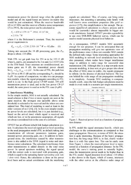
Figure 1. Received power level as a function of propagation
distance
In FPL model the signal attenuates heavily, which sets
challenges to the communications as compared to free
space propagation. However, in terms of MAI, the situation
is quite interesting. Because of the heavy propagation
loss, the long range MAI is, in fact, clearly weaker
than it is with free space loss. This can be easily seen
from Figure 1, where the received power level is represented
as a function of propagation distance. In the FPL
model, the curve's starting point is naturally higher,
since the transmission power needs to be higher than in
the FSL model. Signal detection level (about -110 dBm)
is also shown in the figure, which of course, intersects
with the other curves at the effective radio range of