Database Fundamentals

Database
Fundamentals
A book for the community by the community
Neeraj Sharma, Liviu Perniu, Raul F. Chong, Abhishek Iyer, Chaitali Nandan,
Adi-Cristina Mitea, Mallarswami Nonvinkere, Mirela Danubianu
F I R S T E D I T I O N

Database Fundamentals 4
First Edition (November 2010)
© Copyright IBM Corporation 2010. All rights reserved.
IBM Canada
8200 Warden Avenue
Markham, ON
L6G 1C7
Canada
This edition covers IBM ® DB2 ® Express-C Version 9.7 for Linux ®, UNIX ® and
Windows ® .

5
Notices
This information was developed for products and services offered in the U.S.A.
IBM may not offer the products, services, or features discussed in this document in other countries.
Consult your local IBM representative for information on the products and services currently available
in your area. Any reference to an IBM product, program, or service is not intended to state or imply
that only that IBM product, program, or service may be used. Any functionally equivalent product,
program, or service that does not infringe any IBM intellectual property right may be used instead.
However, it is the user's responsibility to evaluate and verify the operation of any non-IBM product,
program, or service.
IBM may have patents or pending patent applications covering subject matter described in this
document. The furnishing of this document does not grant you any license to these patents. You can
send license inquiries, in writing, to:
IBM Director of Licensing
IBM Corporation
North Castle Drive
Armonk, NY 10504-1785
U.S.A.
For license inquiries regarding double-byte character set (DBCS) information, contact the IBM
Intellectual Property Department in your country or send inquiries, in writing, to:
Intellectual Property Licensing
Legal and Intellectual Property Law
IBM Japan, Ltd.
3-2-12, Roppongi, Minato-ku, Tokyo 106-8711
The following paragraph does not apply to the United Kingdom or any other country where
such provisions are inconsistent with local law: INTERNATIONAL BUSINESS MACHINES
CORPORATION PROVIDES THIS PUBLICATION "AS IS" WITHOUT WARRANTY OF ANY KIND,
EITHER EXPRESS OR IMPLIED, INCLUDING, BUT NOT LIMITED TO, THE IMPLIED
WARRANTIES OF NON-INFRINGEMENT, MERCHANTABILITY OR FITNESS FOR A
PARTICULAR PURPOSE. Some states do not allow disclaimer of express or implied warranties in
certain transactions, therefore, this statement may not apply to you.
This information could include technical inaccuracies or typographical errors. Changes are
periodically made to the information herein; these changes will be incorporated in new editions of the
publication. IBM may make improvements and/or changes in the product(s) and/or the program(s)
described in this publication at any time without notice.
Any references in this information to non-IBM Web sites are provided for convenience only and do
not in any manner serve as an endorsement of those Web sites. The materials at those Web sites
are not part of the materials for this IBM product and use of those Web sites is at your own risk.
IBM may use or distribute any of the information you supply in any way it believes appropriate without
incurring any obligation to you.

Database Fundamentals 6
The licensed program described in this document and all licensed material available for it are
provided by IBM under terms of the IBM Customer Agreement, IBM International Program License
Agreement or any equivalent agreement between us.
Any performance data contained herein was determined in a controlled environment. Therefore, the
results obtained in other operating environments may vary significantly. Some measurements may
have been made on development-level systems and there is no guarantee that these measurements
will be the same on generally available systems. Furthermore, some measurements may have been
estimated through extrapolation. Actual results may vary. Users of this document should verify the
applicable data for their specific environment.
Information concerning non-IBM products was obtained from the suppliers of those products, their
published announcements or other publicly available sources. IBM has not tested those products and
cannot confirm the accuracy of performance, compatibility or any other claims related to non-IBM
products. Questions on the capabilities of non-IBM products should be addressed to the suppliers of
those products.
All statements regarding IBM's future direction or intent are subject to change or withdrawal without
notice, and represent goals and objectives only.
This information contains examples of data and reports used in daily business operations. To
illustrate them as completely as possible, the examples include the names of individuals, companies,
brands, and products. All of these names are fictitious and any similarity to the names and addresses
used by an actual business enterprise is entirely coincidental.
COPYRIGHT LICENSE:
This information contains sample application programs in source language, which illustrate
programming techniques on various operating platforms. You may copy, modify, and distribute these
sample programs in any form without payment to IBM, for the purposes of developing, using,
marketing or distributing application programs conforming to the application programming interface
for the operating platform for which the sample programs are written. These examples have not been
thoroughly tested under all conditions. IBM, therefore, cannot guarantee or imply reliability,
serviceability, or function of these programs. The sample programs are provided "AS IS", without
warranty of any kind. IBM shall not be liable for any damages arising out of your use of the sample
programs.
References in this publication to IBM products or services do not imply that IBM intends to make
them available in all countries in which IBM operates.
If you are viewing this information softcopy, the photographs and color illustrations may not
appear.

7
Trademarks
IBM, the IBM logo, and ibm.com are trademarks or registered trademarks of International Business
Machines Corp., registered in many jurisdictions worldwide. Other product and service names might
be trademarks of IBM or other companies. A current list of IBM trademarks is available on the Web at
“Copyright and trademark information” at www.ibm.com/legal/copytrade.shtml.
Java and all Java-based trademarks are trademarks of Sun Microsystems, Inc. in the United States,
other countries, or both.
Microsoft and Windows are trademarks of Microsoft Corporation in the United States, other countries,
or both.
Linux is a registered trademark of Linus Torvalds in the United States, other countries, or both.
UNIX is a registered trademark of The Open Group in the United States and other countries.
Other company, product, or service names may be trademarks or service marks of others.

Table of Contents
Preface ............................................................................................................................. 15
Who should read this book? ........................................................................................ 15
How is this book structured? ........................................................................................ 15
A book for the community ............................................................................................ 15
Conventions ................................................................................................................. 15
What’s next? ................................................................................................................ 16
About the Authors ........................................................................................................... 17
Contributors .................................................................................................................... 19
Acknowledgements ........................................................................................................ 21
Chapter 1 - Databases and information models .......................................................... 23
1.1 What is a database? .............................................................................................. 23
1.2 What is a database management system? ........................................................... 23
1.2.1 The evolution of database management systems .......................................... 24
1.3 Introduction to information models and data models ............................................. 26
1.4 Types of information models .................................................................................. 27
1.4.1 Network model ................................................................................................ 28
1.4.2 Hierarchical model .......................................................................................... 28
1.4.3 Relational model ............................................................................................. 29
1.4.4 Entity-Relationship model ............................................................................... 30
1.4.5 Object-relational model ................................................................................... 31
1.4.6 Other data models .......................................................................................... 32
1.5 Typical roles and career path for database professionals ..................................... 32
1.5.1 Data Architect ................................................................................................. 32
1.5.2 Database Architect ......................................................................................... 32
1.5.3 Database Administrator (DBA) ....................................................................... 33
1.5.4 Application Developer ..................................................................................... 34
1.6 Summary ................................................................................................................ 34
1.7 Exercises ............................................................................................................... 35
1.8 Review questions ................................................................................................... 35
Chapter 2 – The relational data model .......................................................................... 37
2.1 Relational data model: The big picture .................................................................. 37
2.2 Basic concepts ....................................................................................................... 38
2.2.1 Attributes ......................................................................................................... 38
2.2.2 Domains .......................................................................................................... 39
2.2.3 Tuples ............................................................................................................. 40
2.2.4 Relations ......................................................................................................... 40
2.2.5 Schemas ......................................................................................................... 41
2.2.6 Keys ................................................................................................................ 41
2.3 Relational data model constraints .......................................................................... 44
2.3.1 Entity integrity constraint ................................................................................. 44
2.3.2 Referential integrity constraint ........................................................................ 45
2.3.3 Semantic integrity constraints ......................................................................... 46
2.4 Relational algebra .................................................................................................. 49

Database Fundamentals 10
2.4.1 Union ............................................................................................................... 49
2.4.2 Intersection ..................................................................................................... 49
2.4.3 Difference ....................................................................................................... 50
2.4.4 Cartesian product ........................................................................................... 51
2.4.5 Selection ......................................................................................................... 52
2.4.6 Projection ........................................................................................................ 53
2.4.7 Join ................................................................................................................. 54
2.4.8 Division ........................................................................................................... 56
2.5. Relational calculus ................................................................................................ 57
2.5.1 Tuple-oriented relational calculus ................................................................... 58
2.5.2 Domain-oriented relational calculus ............................................................... 59
2.6 Summary ................................................................................................................ 60
2.7 Exercises ............................................................................................................... 60
2.8 Review questions ................................................................................................... 62
Chapter 3 – The conceptual data model ....................................................................... 65
3.1 Conceptual, logical and physical modeling: The big picture .................................. 65
3.2 What is a model? ................................................................................................... 67
3.2.1 Data model ..................................................................................................... 67
3.2.2 Database model .............................................................................................. 67
3.2.3 Conceptual data model concepts ................................................................... 68
3.3 A case study involving a Library Management System - Part 1 of 3 ..................... 77
3.3.1 Developing the conceptual model .................................................................. 77
3.4 Summary ................................................................................................................ 85
3.5 Exercises ............................................................................................................... 85
3.6 Review questions ................................................................................................... 85
Chapter 4 – Relational Database Design ...................................................................... 89
4.1 The problem of redundancy ................................................................................... 89
4.1.1 Insertion Anomalies ........................................................................................ 90
4.1.2 Deletion Anomalies ......................................................................................... 90
4.1.3 Update Anomalies .......................................................................................... 90
4.2. Decompositions .................................................................................................... 91
4.3. Functional Dependencies ..................................................................................... 92
4.4 Properties of Functional Dependencies ................................................................. 94
4.4.1 Armstrong’s Axioms ........................................................................................ 94
4.4.2 Computing the closure set of attributes .......................................................... 95
4.4.3 Entailment ....................................................................................................... 96
4.5 Normal Forms ........................................................................................................ 96
4.5.1 First Normal Form (1NF) ................................................................................. 96
4.5.2 Second Normal Form (2NF) ........................................................................... 98
4.5.3 Third Normal Form (3NF) ............................................................................... 99
4.5.4 Boyce-Codd Normal Form (BCNF) ............................................................... 100
4.6 Properties of Decompositions .............................................................................. 101
4.6.1 Lossless and Lossy Decompositions ............................................................ 102
4.6.2 Dependency-Preserving Decompositions .................................................... 103
4.7 Minimal Cover ...................................................................................................... 103

4.8 Synthesis of 3NF schemas .................................................................................. 105
4.9 3NF decomposition .............................................................................................. 106
4.10 The Fourth Normal Form (4NF) ......................................................................... 106
4.10.1 Multi-valued dependencies ......................................................................... 107
4.11 Other normal forms ............................................................................................ 108
4.12 A case study involving a Library Management System - Part 2 of 3 ................. 108
4.13 Summary ............................................................................................................ 111
4.14 Exercises ........................................................................................................... 112
4.15 Review questions ............................................................................................... 112
Chapter 5 – Introduction to SQL .................................................................................. 115
5.1 History of SQL ...................................................................................................... 115
5.2 Defining a relational database schema in SQL ................................................... 116
5.2.1 Data Types.................................................................................................... 116
5.2.2 Creating a table ............................................................................................ 117
5.2.3 Creating a schema ........................................................................................ 120
5.2.4 Creating a view ............................................................................................. 121
5.2.5 Creating other database objects ................................................................... 121
5.2.6 Modifying database objects .......................................................................... 121
5.2.7 Renaming database objects ......................................................................... 122
5.3 Data manipulation with SQL ................................................................................ 122
5.3.1 Selecting data ............................................................................................... 122
5.3.2 Inserting data ................................................................................................ 123
5.3.3 Deleting data ................................................................................................. 124
5.3.4 Updating data ............................................................................................... 124
5.4 Table joins ............................................................................................................ 125
5.4.1 Inner joins ..................................................................................................... 125
5.4.2 Outer joins..................................................................................................... 126
5.5 Union, intersection, and difference operations .................................................... 128
5.5.1 Union ............................................................................................................. 129
5.5.2 Intersection ................................................................................................... 130
5.5.3 Difference (Except) ....................................................................................... 130
5.6 Relational operators ............................................................................................. 131
5.6.1 Grouping operators ....................................................................................... 131
5.6.2 Aggregation operators .................................................................................. 132
5.6.3 HAVING Clause ............................................................................................ 132
5.7 Sub-queries .......................................................................................................... 132
5.7.1 Sub-queries returning a scalar value ............................................................ 133
5.7.2 Sub-queries returning vector values ............................................................. 133
5.7.3 Correlated sub-query .................................................................................... 133
5.7.4 Sub-query in FROM Clauses ........................................................................ 134
5.8 Mapping of object-oriented concepts to relational concepts ................................ 134
5.10 A case study involving a Library Management System - Part 3 of 3 ................. 135
5.9 Summary .............................................................................................................. 139
5.10 Exercises ........................................................................................................... 140
5.11 Review questions ............................................................................................... 140
11

Database Fundamentals 12
Chapter 6 – Stored procedures and functions ........................................................... 143
6.1 Working with IBM Data Studio ............................................................................. 143
6.1.1 Creating a project ......................................................................................... 144
6.2 Working with stored procedures .......................................................................... 146
6.2.1 Types of procedures ..................................................................................... 147
6.2.2 Creating a stored procedure ......................................................................... 148
6.2.3 Altering and dropping a stored procedure .................................................... 152
6.3 Working with functions ......................................................................................... 153
6.3.1 Types of functions ......................................................................................... 153
6.3.2 Creating a function ........................................................................................ 154
6.3.3 Invoking a function ........................................................................................ 155
6.3.4 Altering and dropping a function ................................................................... 156
6.4 Summary .............................................................................................................. 157
6.5 Exercises ............................................................................................................. 157
6.6 Review Questions ................................................................................................ 157
Chapter 7 – Using SQL in an application ................................................................... 161
7.1 Using SQL in an application: The big picture ...................................................... 161
7.2 What is a transaction? ......................................................................................... 162
7.3 Embedded SQL ................................................................................................... 163
7.3.1 Static SQL ..................................................................................................... 163
7.3.2 Dynamic SQL ................................................................................................ 168
7.3.3 Static vs. dynamic SQL ................................................................................. 172
7.4 Database APIs ..................................................................................................... 173
7.4.1 ODBC and the IBM Data Server CLI driver .................................................. 173
7.4.2 JDBC ............................................................................................................. 175
7.5 pureQuery ............................................................................................................ 176
7.5.1 IBM pureQuery Client Optimizer ................................................................... 179
7.6 Summary .............................................................................................................. 179
7.7 Exercises ............................................................................................................. 180
7.8 Review Questions ................................................................................................ 180
Chapter 8 – Query languages for XML ........................................................................ 183
8.1 Overview of XML.................................................................................................. 183
8.1.1 XML Elements and Database Objects .......................................................... 183
8.1.2 XML Attributes .............................................................................................. 185
8.1.3 Namespaces ................................................................................................. 186
8.1.4 Document Type Definitions .......................................................................... 187
8.1.5 XML Schema ................................................................................................ 188
8.2 Overview of XML Schema ................................................................................... 189
8.2.1 Simple Types ................................................................................................ 189
8.2.2 Complex Types ............................................................................................. 191
8.2.3 Integrity constraints ....................................................................................... 192
8.2.4 XML Schema evolution ................................................................................. 193
8.3 XPath ................................................................................................................... 194
8.3.1 The XPath data model .................................................................................. 194
8.3.2 Document Nodes .......................................................................................... 194

8.3.3 Path Expressions .......................................................................................... 196
8.3.4 Advanced Navigation in XPath ..................................................................... 196
8.3.5 XPath Semantics .......................................................................................... 196
8.3.6 XPath Queries .............................................................................................. 198
8.4 XQuery ................................................................................................................. 199
8.4.1 XQuery basics .............................................................................................. 200
8.4.2 FLWOR expressions ..................................................................................... 200
8.4.3 Joins in XQuery ............................................................................................ 201
8.4.4 User-defined functions .................................................................................. 202
8.4.5 XQuery and XML Schema ............................................................................ 202
8.4.6 Grouping and aggregation ............................................................................ 202
8.4.7 Quantification ................................................................................................ 204
8.5 XSLT .................................................................................................................... 204
8.6 SQL/XML ............................................................................................................. 206
8.6.1 Encoding relations as XML Documents ........................................................ 206
8.6.2 Storing and publishing XML documents ....................................................... 207
8.6.3 SQL/XML Functions ...................................................................................... 207
8.7 Querying XML documents stored in tables .......................................................... 211
8.8 Modifying data ...................................................................................................... 212
8.8.1 XMLPARSE .................................................................................................. 212
8.8.2 XMLSERIALIZE ............................................................................................ 213
8.8.3 The TRANSFORM expression ..................................................................... 213
8.9 Summary .............................................................................................................. 214
8.10 Exercises ........................................................................................................... 215
8.11 Review questions ............................................................................................... 215
Chapter 9 – Database Security .................................................................................... 221
9.1 Database security: The big picture ...................................................................... 221
9.1.1 The need for database security .................................................................... 222
9.1.2 Access control .............................................................................................. 224
9.1.3 Database security case study ....................................................................... 225
9.1.4 Views ............................................................................................................ 231
9.1.5 Integrity Control ............................................................................................ 231
9.1.6 Data encryption ............................................................................................. 231
9.2 Security policies and procedures ......................................................................... 232
9.2.1 Personnel control .......................................................................................... 232
9.2.2 Physical access control ................................................................................ 232
9.3 Summary .............................................................................................................. 233
9.4 Exercises ............................................................................................................. 233
9.5 Review Questions ................................................................................................ 233
Chapter 10 – Technology trends and databases ....................................................... 235
10.1 What is Cloud computing? ................................................................................. 235
10.1.1 Characteristics of the Cloud ........................................................................ 236
10.1.2 Cloud computing service models ................................................................ 237
10.1.3 Cloud providers ........................................................................................... 237
10.1.4 Handling security on the Cloud ................................................................... 241
13

Database Fundamentals 14
10.1.5 Databases and the Cloud ........................................................................... 242
10.2 Mobile application development ........................................................................ 243
10.2.1 Developing for a specific device ................................................................. 244
10.2.2 Developing for an application platform ....................................................... 245
10.2.3 Mobile device platform ................................................................................ 246
10.2.4 Mobile application development platform ................................................... 247
10.2.5 The next wave of mobile applications ......................................................... 248
10.2.6 DB2 Everyplace .......................................................................................... 248
10.3 Business intelligence and appliances ................................................................ 249
10.4 db2university.com: Implementing an application on the Cloud (case study)..... 249
10.4.1 Moodle open source course management system ..................................... 250
10.4.2 Enabling openID sign-in.............................................................................. 253
10.4.3 Running on the Amazon Cloud ................................................................... 254
10.4.4 Using an Android phone to retrieve course marks ..................................... 255
10.5 Summary ............................................................................................................ 256
Appendix A – Solutions to review questions ............................................................. 259
Appendix B – Up and running with DB2 ..................................................................... 264
B.1 DB2: The big picture ............................................................................................ 264
B.2 DB2 Packaging .................................................................................................... 265
B.2.1 DB2 servers .................................................................................................. 265
B.2.2 DB2 Clients and Drivers ............................................................................... 266
B.3 Installing DB2 ...................................................................................................... 267
B.3.1 Installation on Windows................................................................................ 267
B.3.2 Installation on Linux ...................................................................................... 268
B.4 DB2 tools ............................................................................................................. 268
B.4.1 Control Center .............................................................................................. 268
B.4.2 Command Line Tools ................................................................................... 270
B.5 The DB2 environment ......................................................................................... 273
B.6 DB2 configuration ................................................................................................ 274
B.7 Connecting to a database ................................................................................... 275
B.8 Basic sample programs ....................................................................................... 276
B.9 DB2 documentation ............................................................................................. 278
Resources ...................................................................................................................... 279
Web sites ................................................................................................................... 279
Books ......................................................................................................................... 279
References ................................................................................................................. 280
Contact ....................................................................................................................... 281

Preface
Keeping your skills current in today's world is becoming increasingly challenging. There are
too many new technologies being developed, and little time to learn them all. The DB2® on
Campus Book Series has been developed to minimize the time and effort required to learn
many of these new technologies.
This book helps new database professionals understand database concepts with the right
blend of breadth and depth of information.
Who should read this book?
This book is tailored for new database enthusiasts, application developers, database
administrators, and anyone with an interest in the subject and looking to get exposure such
as university students and new graduates.
How is this book structured?
This book is divided into chapters, starting with the basic database concepts and
information models in Chapter 1. Chapter 2 covers relational data models. Chapter 3 and 4
explain conceptual modeling and relational database design. In Chapters 5, 6 and 7 the
focus is geared towards SQL. Chapter 8 highlights XML data storage and retrieval via SQL
and XQuery. Chapter 9 addresses database security aspects. The book then concludes
with an overview of various other key technologies and relevant applications that are
increasingly popular in the industry today.
Exercises and review questions can be found with most chapters. The solutions have been
provided in Appendix A.
A book for the community
This book was created by a community of university professors, students, and
professionals (including IBM employees). Members from around the world have
participated in developing this book. The online version of this book is released to the
community at no charge. If you would like to provide feedback, contribute new material,
improve existing material, or help with translating this book to another language, please
send an email of your planned contribution to db2univ@ca.ibm.com with the subject
“Database fundamentals book feedback”.
Conventions
Many examples of commands, SQL statements, and code are included throughout the
book. Specific keywords are written in uppercase bold. For example: A NULL represents an
unknown state. Commands are shown in lowercase bold. For example: The dir
command lists all files and subdirectories on Windows. SQL statements are shown in

Database Fundamentals 16
upper case bold. For example: Use the SELECT statement to retrieve information from a
table.
Object names used in our examples are shown in bold italics. For example: The flights
table has five columns.
Italics are also used for variable names in the syntax of a command or statement. If the
variable name has more than one word, it is joined with an underscore. For example:
CREATE TABLE table_name
What’s next?
We recommend that you review the following books in this book series for more details
about related topics:
• Getting started with DB2 Express-C
• Getting started with InfoSphere Data Architect
• Getting started with data warehousing
• Getting started with DB2 application development
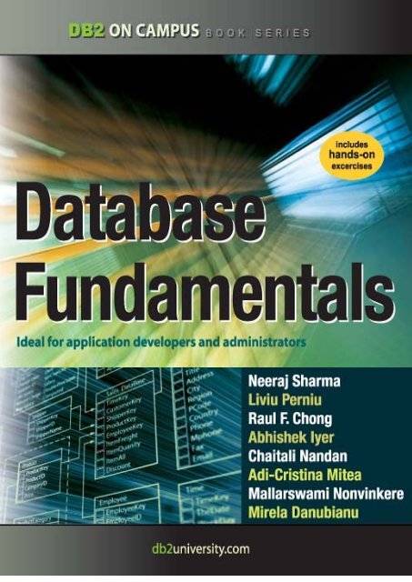
The following figure shows all the different eBooks in the DB2 on Campus book series
available free at db2university.com
The DB2 on Campus book series

17
About the Authors
Neeraj Sharma is a senior IT specialist at the Dynamic Warehousing Center of
Competency, IBM India Software Labs. His primary role is design, configuration and
implementation of large data warehouses across various industry domains; implementation
of custom proof of concept (POC) exercises, and execution of performance benchmarks at
customer's request. He holds a bachelor’s degree in electronics and communication
engineering and a master’s degree in software systems.
Liviu Perniu is an Associate Professor in the Automation Department at Transilvania
University of Brasov, Romania, teaching courses in the area of Data Requirements,
Analysis, and Modeling. He is an IBM 2006 Faculty Award recipient as part of the Eclipse
Innovation Awards program.
Raul F. Chong is the DB2 on Campus program manager based at the IBM Toronto
Laboratory, and a DB2 technical evangelist. His main responsibility is to grow the DB2
community around the world. Raul joined IBM in 1997 and has held numerous positions in
the company. As a DB2 consultant, Raul helped IBM business partners with migrations
from other relational database management systems to DB2, as well as with database
performance and application design issues. As a DB2 technical support specialist, Raul
has helped resolve DB2 problems on the OS/390®, z/OS®, Linux®, UNIX® and Windows
platforms. Raul has taught many DB2 workshops, has published numerous articles, and
has contributed to the DB2 Certification exam tutorials. Raul has summarized many of his
DB2 experiences through the years in his book Understanding DB2 - Learning Visually with
Examples 2nd Edition (ISBN-10: 0131580183) for which he is the lead author. He has also
co-authored the book DB2 SQL PL Essential Guide for DB2 UDB on Linux, UNIX,
Windows, i5/OS, and z/OS (ISBN 0131477005), and is the project lead and co-author of
many of the books in the DB2 on Campus book series.
Abhishek Iyer is an engineer at the Warehousing Center of Competency, IBM India
Software Laboratory. His primary role is to create proof of concepts and execute
performance benchmarks on customer requests. His expertise includes data warehouse
implementation and data mining. He holds a bachelor’s degree in computer science.
Chaitali Nandan is a software engineer working in the DB2 Advanced Technical Support
team based at the IBM India Software Laboratory. Her primary role is to provide first relief
and production support to DB2 Enterprise customers. She specializes in critical problem
solving skills for DB2 production databases. She holds a Bachelor of Engineering degree in
Information Technology.
Adi-Cristina Mitea is an associate professor at the Computer Science Department,
“Hermann Oberth” Faculty of Engineering, “Lucian Blaga” University of Sibiu, Romania.
She teaches courses in the field of databases, distributed systems, parallel and distributed
algorithms, fault tolerant systems and others. Her research activities are in these same
areas. She holds a bachelor’s degree and a Ph.D in computer science.

Database Fundamentals 18
Mallarswami Nonvinkere is a pureXML® specialist with IBM’s India Software Laboratory
and works for the DB2 pureXML enablement team in India. He works with IBM customers
and ISVs to help them understand the use of pureXML technology and develop high
performance applications using XML. Mallarswami helps customers with best practices and
is actively involved in briefing customers about DB2 related technologies. He has been a
speaker at various international conferences including IDUG Australasia, IDUG India and
IMTC and has presented at various developerWorks ® forums.
Mirela Danubianu is a lecturer at Stefan cel Mare University of Suceava, Faculty of
Electrical Engineering and Computer Science. She received a MS in Computer Science at
University of Craiova (1985 – Automatizations and Computers) and other in Economics at
Stefan cel Mare University of Suceava, (2009 - Management). She holds a PhD in
Computers Science from Stefan cel Mare University of Suceava (2006 - Contributions to
the development of data mining and knowledge methods and techniques). Her current
research interests include databases theory and implementation, data mining and data
warehousing, application of advanced information technology in economics and health care
area. Mirela has co-authored 7 books and more than 25 papers. She has participated in
more than 15 conferences, and is a member of the International Program Committee in
three conferences.

Contributors
The following people edited, reviewed, provided content, and contributed significantly to
this book.
Contributor Company/University Position/Occupation Contribution
Agatha
Colangelo
ION Designs, Inc Data Modeler Developed the core
table of contents of the
book
Cuneyt Goksu
VBT Vizyon Bilgi
Teknolojileri
DB2 SME and IBM
Gold Consultant
Technical review
Marcus
Graham
IBM US Software developer English and technical
review of Chapter 10
Amna Iqbal IBM Toronto Lab Quality Assurance -
Lotus Foundations
English review of the
entire book except
chapters 5 and 7
Leon
Katsnelson
IBM Toronto Lab
Program Director, IBM
Data Servers
Technical review, and
contributor to Chapter
10 content
Jeff (J.Y.) Luo IBM Toronto Lab Technical Enablement
Specialist
English review of
chapter 7
Fraser
McArthur
IBM Toronto Lab
Information
Management
Evangelist
Technical review
Danna
Nicholson
IBM US
STG ISV Enablement,
Web Services
English review of the
entire book.
Rulesh
Rebello
IBM India Advisory Manager -
IBM Software Group
Client Support
Technical review
Suresh Sane DST Systems, Inc Database Architect Review of various
chapters, especially
those related to SQL
Nadim Sayed IBM Toronto Lab User-Centered Design
Specialist
English review of
chapter 1

Database Fundamentals 20
Ramona Truta University of Toronto Lecturer Developed the core
table of contents of the
book.

Acknowledgements
We greatly thank the following individuals for their assistance in developing materials
referenced in this book.
Natasha Tolub for designing the cover of this book.
Susan Visser for assistance with publishing this book.

1
Chapter 1 - Databases and information models
Data is one of the most critical assets of any business. It is used and collected practically
everywhere, from businesses trying to determine consumer patterns based on credit card
usage, to space agencies trying to collect data from other planets. Data, as important as it
is, needs robust, secure, and highly available software that can store and process it
quickly. The answer to these requirements is a solid and a reliable database.
Database software usage is pervasive, yet it is taken for granted by the billions of daily
users worldwide. Its presence is everywhere-from retrieving money through an automatic
teller machine to badging access at a secure office location.
This chapter provides you an insight into the fundamentals of database management
systems and information models.
1.1 What is a database?
Since its advent, databases have been among the most researched knowledge domains in
computer science. A database is a repository of data, designed to support efficient data
storage, retrieval and maintenance. Multiple types of databases exist to suit various
industry requirements. A database may be specialized to store binary files, documents,
images, videos, relational data, multidimensional data, transactional data, analytic data, or
geographic data to name a few.
Data can be stored in various forms, namely tabular, hierarchical and graphical forms. If
data is stored in a tabular form then it is called a relational database. When data is
organized in a tree structure form, it is called a hierarchical database. Data stored as
graphs representing relationships between objects is referred to as a network database.
In this book, we focus on relational databases.
1.2 What is a database management system?
While a database is a repository of data, a database management system, or simply
DBMS, is a set of software tools that control access, organize, store, manage, retrieve and
maintain data in a database. In practical use, the terms database, database server,

Database Fundamentals 24
database system, data server, and database management systems are often used
interchangeably.
Why do we need database software or a DBMS? Can we not just store data in simple text
files for example? The answer lies in the way users access the data and the handle of
corresponding challenges. First, we need the ability to have multiple users insert, update
and delete data to the same data file without "stepping on each other's toes". This means
that different users will not cause the data to become inconsistent, and no data should be
inadvertently lost through these operations. We also need to have a standard interface for
data access, tools for data backup, data restore and recovery, and a way to handle other
challenges such as the capability to work with huge volumes of data and users. Database
software has been designed to handle all of these challenges.
The most mature database systems in production are relational database management
systems (RDBMS’s). RDBMS's serve as the backbone of applications in many industries
including banking, transportation, health, and so on. The advent of Web-based interfaces
has only increased the volume and breadth of use of RDBMS, which serve as the data
repositories behind essentially most online commerce.
1.2.1 The evolution of database management systems
In the 1960s, network and hierarchical systems such as CODASYL and IMSTM were the
state-of-the-art technology for automated banking, accounting, and order processing
systems enabled by the introduction of commercial mainframe computers. While these
systems provided a good basis for the early systems, their basic architecture mixed the
physical manipulation of data with its logical manipulation. When the physical location of
data changed, such as from one area of a disk to another, applications had to be updated
to reference the new location.
A revolutionary paper by E.F. Codd, an IBM San Jose Research Laboratory employee in
1970, changed all that. The paper titled “A relational model of data for large shared data
banks” [1.1] introduced the notion of data independence, which separated the physical
representation of data from the logical representation presented to applications. Data could
be moved from one part of the disk to another or stored in a different format without
causing applications to be rewritten. Application developers were freed from the tedious
physical details of data manipulation, and could focus instead on the logical manipulation of
data in the context of their specific application.
Figure 1.1 illustrates the evolution of database management systems.

Chapter 1 - Databases and information models 25
Figure 1.1 Evolution of database management systems
The above figure describes the evolution of database management systems with the
relational model that provide for data independence. IBM's System R was the first system
to implement Codd's ideas. System R was the basis for SQL/DS, which later became DB2.
It also has the merit to introduce SQL, a relational database language used as a standard
today, and to open the door for commercial database management systems.
Today, relational database management systems are the most used DBMS's and are
developed by several software companies. IBM is one of the leaders in the market with
DB2 database server. Other relational DBMS's include Oracle, Microsoft SQL Server,
INGRES, PostgreSQL, MySQL, and dBASE.
As relational databases became increasingly popular, the need to deliver high performance
queries has arisen. DB2's optimizer is one of the most sophisticated components of the
product. From a user's perspective, you treat DB2's optimizer as a black box, and pass any
SQL query to it. The DB2's optimizer will then calculate the fastest way to retrieve your
data by taking into account many factors such as the speed of your CPU and disks, the
amount of data available, the location of the data, the type of data, the existence of
indexes, and so on. DB2's optimizer is cost-based.
As increased amounts of data were collected and stored in databases, DBMS's scaled. In
DB2 for Linux, UNIX and Windows, for example, a feature called Database Partitioning
Feature (DPF) allows a database to be spread across many machines using a sharednothing
architecture. Each machine added brings its own CPUs and disks; therefore, it is
easier to scale almost linearly. A query in this environment is parallelized so that each
machine retrieves portions of the overall result.
Next in the evolution of DBMS's is the concept of extensibility. The Structured Query
Language (SQL) invented by IBM in the early 1970's has been constantly improved
through the years. Even though it is a very powerful language, users are also empowered

Database Fundamentals 26
to develop their own code that can extend SQL. For example, in DB2 you can create userdefined
functions, and stored procedures, which allow you to extend the SQL language
with your own logic.
Then DBMS's started tackling the problem of handling different types of data and from
different sources. At one point, the DB2 data server was renamed to include the term
"Universal" as in "DB2 universal database" (DB2 UDB). Though this term was later
dropped for simplicity reasons, it did highlight the ability that DB2 data servers can store all
kinds of information including video, audio, binary data, and so on. Moreover, through the
concept of federation a query could be used in DB2 to access data from other IBM
products, and even non-IBM products.
Lastly, in the figure the next evolutionary step highlights integration. Today many
businesses need to exchange information, and the eXtensible Markup Language (XML) is
the underlying technology that is used for this purpose. XML is an extensible, selfdescribing
language. Its usage has been growing exponentially because of Web 2.0, and
service-oriented architecture (SOA). IBM recognized early the importance of XML;
therefore, it developed a technology called pureXML ® that is available with DB2 database
servers. Through this technology, XML documents can now be stored in a DB2 database in
hierarchical format (which is the format of XML). In addition, the DB2 engine was extended
to natively handle XQuery, which is the language used to navigate XML documents. With
pureXML, DB2 offers the best performance to handle XML, and at the same time provides
the security, robustness and scalability it has delivered for relational data through the
years.
The current "hot" topic at the time of writing is Cloud Computing. DB2 is well positioned to
work on the Cloud. In fact, there are already DB2 images available on the Amazon EC2
cloud, and on the IBM Smart Business Development and Test on the IBM Cloud (also
known as IBM Development and Test Cloud). DB2's Database Partitioning Feature
previously described fits perfectly in the cloud where you can request standard nodes or
servers on demand, and add them to your cluster. Data rebalancing is automatically
performed by DB2 on the go. This can be very useful during the time when more power
needs to be given to the database server to handle end-of-the-month or end-of-the-year
transactions.
1.3 Introduction to information models and data models
An information model is an abstract, formal representation of entities that includes their
properties, relationships and the operations that can be performed on them. The entities
being modeled may be from the real world, such as devices on a network, or they may
themselves be abstract, such as the entities used in a billing system.
The primary motivation behind the concept is to formalize the description of a problem
domain without constraining how that description will be mapped to an actual
implementation in software. There may be many mappings of the Information Model. Such
mappings are called data models, irrespective of whether they are object models (for

Chapter 1 - Databases and information models 27
example, using unified modeling language - UML), entity relationship models, or XML
schemas.
Modeling is important as it considers the flexibility required for possible future changes
without significantly affecting usage. Modeling allows for compatibility with its predecessor
models and has provisions for future extensions.
Information Models and Data Models are different because they serve different purposes.
The main purpose of an Information Model is to model managed objects at a conceptual
level, independent of any specific implementations or protocols used to transport the data.
The degree of detail of the abstractions defined in the Information Model depends on the
modeling needs of its designers. In order to make the overall design as clear as possible,
an Information Model should hide all protocol and implementation details. Another
important characteristic of an Information Model is that it defines relationships between
managed objects.
Data Models, on the other hand, are defined at a more concrete level and include many
details. They are intended for software developers and include protocol-specific constructs.
A data model is the blueprint of any database system. Figure 1.1 illustrates the relationship
between an Information Model and a Data Model.
Information Model
Conceptual/abstract model
for designers and operators
Data Model Data Model Data Model
Concrete/detailed model
for implementors
Figure 1.1 - Relationship between an Information Model and a Data Model
Since conceptual models can be implemented in different ways, multiple Data Models can
be derived from a single Information Model.
1.4 Types of information models
Information model proposals can be split into nine historical epochs:
• Network (CODASYL): 1970’s
• Hierarchical (IMS): late 1960’s and 1970’s
• Relational: 1970’s and early 1980’s
• Entity-Relationship: 1970’s
• Extended Relational: 1980’s

Database Fundamentals 28
• Semantic: late 1970’s and 1980’s
• Object-oriented: late 1980’s and early 1990’s
• Object-relational: late 1980’s and early 1990’s
• Semi-structured (XML): late 1990’s to the present
The next sections discuss some of these models in more detail.
1.4.1 Network model
In 1969, CODASYL (Committee on Data Systems Languages) released its first
specification about the network data model. This followed in 1971 and 1973 with
specifications for a record-at-a-time data manipulation language. An example of the
CODASYL network data model is illustrated in Figure 1.2.
Figure 1.2 - A network model
The figure shows the record types represented by rectangles. These record types can also
use keys to identify a record. A collection of record types and keys form a CODASYL
network or CODASYL database. Note that a child can have more than one parent, and that
each record type can point to each other with next, prior and direct pointers.
1.4.2 Hierarchical model
The hierarchical model organizes its data using a tree structure. The root of the tree is the
parent followed by child nodes. A child node cannot have more than one parent, though a
parent can have many child nodes. This is depicted in Figure 1.3

Chapter 1 - Databases and information models 29
Figure 1.3 - A Hierarchical model
In a hierarchical model, a collection of named fields with their associated data types is
called a record type. Each instance of a record type is forced to obey the data description
indicated in the definition of the record type. Some fields in the record type are keys.
The first hierarchical database management system was IMS (Information Management
System) released by IBM in 1968. It was originally built as the database for the Apollo
space program to land the first humans on the moon. IMS is a very robust database that is
still in use today at many companies worldwide.
1.4.3 Relational model
The relational data model is simple and elegant. It has a solid mathematic foundation
based on sets theory and predicate calculus and is the most used data model for
databases today.
One of the drivers for Codd's research was the fact that IMS programmers were spending
large amounts of time doing maintenance on IMS applications when logical or physical
changes occurred; therefore, his goal was to deliver a model that provided better data
independence. His proposal was threefold:
• Store the data in a simple data structure (tables)
• Access it through a high level set-at-a-time Data Manipulation Language (DML)
• Be independent from physical storage
With a simple data structure, one has a better chance of providing logical data
independence. With a high-level language, one can provide a high degree of physical data
independence. Therefore, this model allows also for physical storage independence. This
was not possible in either IMS or CODASYL. Figure 1.4 illustrates an example showing an
Entity-Relationship (E-R) diagram that represents entities (tables) and their relationships
for a sample relational model. We discuss more about E-R diagrams in the next section.

Database Fundamentals 30
Figure 1.4 - An E-R diagram showing a sample relational model
1.4.4 Entity-Relationship model
In the mid 1970’s, Peter Chen proposed the entity-relationship (E-R) data model. This was
to be an alternative to the relational, CODASYL, and hierarchical data models. He
proposed thinking of a database as a collection of instances of entities. Entities are objects
that have an existence independent of any other entities in the database. Entities have
attributes, which are the data elements that characterize the entity. One or more of these
attributes could be designated to be a key. Lastly, there could be relationships between
entities. Relationships could be 1-to-1, 1-to-n, n-to-1 or m-to-n, depending on how the
entities participated in the relationship. Relationships could also have attributes that
described the relationship. Figure 1.5 provides an example of an E-R diagram.

Chapter 1 - Databases and information models 31
Figure 1.5 - An E-R Diagram for a telephone directory data model
In the figure, entities are represented by rectangles and they are name, address, voice,
fax, and modem. Attributes are listed inside each entity. For example, the voice entity has
the vce_num, rec_num, and vce-type as attributes. PK represents a primary key, and
FK a foreign key. The concept of keys is discussed in more detail later in this book.
Rather than being used as a model on its own, the E-R model has found success as a tool
to design relational databases. Chen’s papers contained a methodology for constructing an
initial E-R diagram. In addition, it was a simple process to convert an E-R diagram into a
collection of tables in third normal form. For more information on the Third normal form and
the normalization theory see the later parts of the book.
Today, the ability to create E-R diagrams are incorporated into data modeling tools such as
IBM InfoSphere Data Architect. To learn more about this tool refer to the eBook Getting
started with InfoSphere Data Architect, which is part of the DB2 on Campus book series.
1.4.5 Object-relational model
The Object-Relational (OR) model is very similar to the relational model; however, it treats
every entity as an object (instance of a class), and a relationship as an inheritance. Some
features and benefits of an Object-Relational model are:
• Support for complex, user defined types
• Object inheritance
• Extensible objects
Object-Relational databases have the capability to store object relationships in relational
form.

Database Fundamentals 32
1.4.6 Other data models
The last decade has seen a substantial amount of work on semi-structured, semantic and
object oriented data models.
XML is ideal to store semi-structured data. XML-based models have gained a lot of
popularity in the industry thanks to Web 2.0 and service-oriented architecture (SOA).
Object oriented data models are popular in universities, but have not been widely accepted
in the industry; however, object-relational mapping (ORM) tools are available which allow a
seamless integration of object-oriented programs with relational databases.
1.5 Typical roles and career path for database professionals
Like any other work profile, the database domain has several of roles and career paths
associated with it. The following is a description of some of these roles.
1.5.1 Data Architect
A data architect is responsible for designing an architecture that supports the organization's
existing and future needs for data management. The architecture should cover databases,
data integration and the means to get to the data. Usually the data architect achieves his
goals by setting enterprise data standards. A Data Architect is also referred to as a Data
Modeler. This is in spite of the fact that the role involves much more than just creating data
models.
Some fundamental skills of a Data Architect are:
• Logical Data modeling
• Physical Data modeling
• Development of a data strategy and associated policies
• Selection of capabilities and systems to meet business information needs
1.5.2 Database Architect
This role is similar to a Data Architect, though constraints more towards a database
solution. A database architect is responsible for the following activities:
• Gather and document requirements from business users and management and
address them in a solution architecture.
• Share the architecture with business users and management.
• Create and enforce database and application development standards and
processes.
• Create and enforce service level agreements (SLAs) for the business, specially
addressing high availability, backup/restore and security.

Chapter 1 - Databases and information models 33
• Study new products, versions compatibility, and deployment feasibility and give
recommendations to development teams and management.
• Understand hardware, operating system, database system, multi-tier component
architecture and interaction between these components.
• Prepare high-level documents in-line with requirements.
• Review detailed designs and implementation details.
It is critical for a database architect to keep pace with the various tools, database products,
hardware platforms and operating systems from different vendors as they evolve and
improve.
1.5.3 Database Administrator (DBA)
A database administrator (DBA) is responsible for the maintenance, performance, integrity
and security of a database. Additional role requirements are likely to include planning,
development and troubleshooting.
The work of a database administrator (DBA) varies according to the nature of the
employing organization and the level of responsibility associated with the post. The work
may be pure maintenance or it may also involve specializing in database development.
Typical responsibilities include some or all of the following:
• Establishing the needs of users and monitoring user access and security;
• Monitoring performance and managing parameters to provide fast query responses
to front-end users;
• Mapping out the conceptual design for a planned database in outline;
• Take into account both, back-end organization of data and front-end accessibility for
end users;
• Refining the logical design so that it can be translated into a specific data model;
• Further refining the physical design to meet system storage requirements;
• Installing and testing new versions of the database management system (DBMS);
• Maintaining data standards, including adherence to the Data Protection Act;
• Writing database documentation, including data standards, procedures and
definitions for the data dictionary (metadata);
• Controlling access permissions and privileges;
• Developing, managing and testing backup and recovery plans;
• Ensuring that storage, archiving, backup and recovery procedures are functioning
correctly;
• Capacity planning;

Database Fundamentals 34
• Working closely with IT project managers, database programmers and Web
developers;
• Communicating regularly with technical, applications and operational staff to ensure
database integrity and security;
• Commissioning and installing new applications.
Because of the increasing levels of hacking and the sensitive nature of data stored,
security and recoverability or disaster recovery have become increasingly important
aspects.
1.5.4 Application Developer
A database application developer is a person in charge of developing applications that
access databases. An application developer requires knowledge of the following:
• Integrated database application development environments (IDEs).
• Database plug-ins for IDEs.
• SQL development tools
• Database performance monitoring and debugging
• Application server environments, application deployment, application performance
monitoring and debugging
An example of an IDE is IBM Data Studio, a free Eclipse-based environment which allows
developers to work with DB2 objects such as tables, views, indexes, stored procedures,
user-defined functions and Web services. It also provides facilities for debugging,
development of SQL and XQuery, and integration with different application servers such as
WebSphere ® Application Server.
DB2 also includes add-ins that extend Microsoft ® Visual Studio development environment
with a comprehensive set of tools for developing DB2 objects (tables, views, stored
procedures, user-defined functions etc.). This way, .NET developers do not need to switch
back and forth between Microsoft Visual Studio and DB2 tools.
The roles and responsibilities discussed so far are very broad classifications. Different
organizations have their own definition of roles within their organization’s context. These
roles are listed to provide a big picture on various dimensions around database
administration, application development and usage.
1.6 Summary
In this chapter, we discussed several database fundamental concepts starting with simple
definitions of a database and extending to a database management system. Then, we
discussed information and data models such as the network, hierarchical, and relational
models. At the end of the chapter, various roles associated with the database domain were
discussed. In the upcoming chapters we will discuss database concepts in more detail.

Chapter 1 - Databases and information models 35
1.7 Exercises
1. Learn more about databases by practicing with DB2 Express-C, the free version of
DB2 database server. You can download this product at ibm.com/db2/express
2. Learn more about IDEs by practicing with the free IBM Data Studio. You can
download this product also at ibm.com/db2/express
1.8 Review questions
1. What is a database?
2. What is a database management system?
3. What is the difference between an Information model, and a Data model?
4. What is the main advantage of the relational model versus other models?
5. List two common tasks a DBA has to perform
6. Which of the following is not an information model:
1. A. pureXML model
2. B. Relational model
3. C. Hierarchical model
4. D. Network model
5. E. None of the above
7. In the evolution of database management systems, what does optimization refer to?
6. A. High availability
7. B. Security
8. C. Performance
9. D. Scalability
10. E. None of the above
8. Which of the following is not listed in the evolution of database management systems:
11. A. Distribution
12. B. Data Independence
13. C. Integration
14. D. Federation
15. E. None of the above
9. In the evolution of database management systems, in which stage would pureXML be?
16. A. Data independence

Database Fundamentals 36
17. B. Extensibility
18. C. Optimization
19. D. Integration
20. E. None of the above
10. What is one key differentiator of DB2 on the Cloud?
21. A. It has a spatial extender
22. B. Its Database Partitioning Feature
23. C. Its pureXML technology
24. D. All of the above
25. E. None of the above

2
Chapter 2 – The relational data model
In this chapter, we discuss the basics of the relational data model. We introduce concepts
like attributes, tuples, relations, domains, schemas and keys. We also describe the
different types of relational model constraints and some information about relational
algebra and calculus. This chapter is closely related to Chapter 3, The conceptual data
model, where you will learn how to translate a conceptual data model into a relational
database schema, and to Chapter 4, Relational database design, which presents important
issues for designing a relational database. This chapter is also important for a better
understanding of the SQL language.
In this chapter, you will learn about:
• The big picture of the relational data model
• The definitions of attributes, tuples, relations, domains, schemas and keys
• The relational model constraints
• Relational algebra operations
• Relational calculus
2.1 Relational data model: The big picture
Information models try to put the real-world information complexity in a framework that can
be easily understood. Data models must capture data structure and characteristics, the
relationships between data, the data validation rules and constraints and all
transformations the data must support. You can think of it as a communication tool
between designers, programmers and end-users of a database. There are several types of
data models on the market today and each of it has its own features. However, in this
chapter we focus on the relational data model, which is the prevalent one in today's
database market.
We present the main aspects of the relational data model below in Figure 2.1.

Database Fundamentals 38
Information Models
The Relational Data Model
Concepts
Attributes
Tuples
Relations
Domains
Schemas
Keys
Constraints
Entity
integrity
Referential
integrity
Semantic
constraints
Relational
Algebra
Relational
Calculus
The
Hierarchical
Data Model
The Network
Data Model
The Object –
Relational
Data Model
Figure 2.1 - Relational data model in context of information models: The big picture
Figure 2.1 shows the main aspects of the relational data model:
• Specific relational data model concepts like attributes, tuples, domains, relations,
domains, schemas, keys
• The relational data model constraints like entity integrity, referential integrity, and
semantic constraints which are used to enforce rules on a relational database
• Relational algebra operations like union, intersection, difference, Cartesian
product, selection, projection, join and division which are used to manipulate
relations in a relational data model
• Relational calculus which is an alternative to the relational algebra as a candidate
for the manipulative part of the model
2.2 Basic concepts
The relational data model uses formal terms to define its concepts. In the following
chapters, we use formal relational terminology like: attribute, domain, tuple, relation,
schema, candidate key, primary key and foreign key. Let’s define each of these terms.
2.2.1 Attributes
An attribute is a characteristic of data. A real-world data feature, modeled in the database,
will be represented by an attribute. An attribute has to have a name, so you can refer to

Chapter 2 – The relational data model 39
that feature, and the name has to be as relevant as possible for that feature. For example,
for a person the attributes can be: Name, Sex, DateOfBirth. Informal terms used to
define an attribute are: column in a table or field in a data file.
In Figure 2.2, you can see the attributes of a car: Type, Producer, Model,
FabricationYear, Color, Fuel. Other elements in the figure as discussed in the
upcoming sections.
CARS Relation
Attribute
Header
TYPE
PRODUCER
MODEL
FABRICATION
YEAR
COLOR
FUEL
LIMOUSINE
BMV
740
2008
BLACK
GAS
VAN
VW
TRANSPORTER
2007
RED
DIESEL
Tuple
Body
LIMOUSIN
MERCEDES
320
2008
WHITE
GAS
LIMOUSINE
AUDI
ALLROAD
2009
BLUE
DIESEL
LIMOUSINE
BMW
525
2007
GREY
DIESEL
Value
Figure 2.2 - CARS Relation – Header with attributes and body with tuples
2.2.2 Domains
A domain is a set of atomic values that are all of the same type. A value is the smallest
unit of data in the relational model. For example, BMW, Mercedes, Audi, and VW are
values for the attribute Producer. Those values are considered to be atomic, that is they
are non-decomposable as far as the model is concerned. The domain for the Producer is
the set of all possible car producer names. An attribute always has a domain associated
with it. This domain gives the possible values for that attribute. Two or more attributes can
be defined on the same domain.
A domain has a name, so we can make references to it, and a dimension. The dimension
is given by the number of values that domain has. For example, Fuel attribute domain
has only two values (GAS, DIESEL). A domain can be seen as a pool of values, from
which the actual values appearing in attributes are drawn. Note that at any given time,
there will be values included in a domain that do not currently appear in any of the
attributes that correspond to that domain.
Domains have a certain operational significance. If two attributes draw their values from the
same domain, then the comparisons operations involving those two attributes make sense
as they are comparing similar values. Conversely, if two attributes draw their values from

Database Fundamentals 40
different domains, comparisons operations involving those two attributes do not make
sense.
Domains are primarily conceptual in nature. In most cases, they are not explicitly stored in
the database. The domains should be specified as a part of the database definition and
then each attribute definition should include a reference to the corresponding domain, so
that the system is aware of those attributes that are comparable to each other.
A given attribute may have the same name as the corresponding domain, but this situation
should be avoided because it can generate confusion. However, it is possible to include the
domain name as the trailing portion of the attribute name for the purpose of including more
information in that attribute name.
2.2.3 Tuples
A tuple is an ordered set of values that describe data characteristics at one moment in
time. In Figure 2.2 above, you can see an example of a tuple. Another formal term used to
define a tuple is n-tuple. Informal terms used for tuples are: row in a table or record in a
data file.
2.2.4 Relations
A relation is the core of the relational data. According to introduction to database systems
[2.1] a relation on domains D1, D2, …, Dn (not necessarily distinct) consists of a
heading and a body.
The heading consists of a fixed set of attributes A1, A2, …, An, such that each attribute
Ai corresponds to exactly one of the underlying domains Di (i=1, 2, …, n).
The body consists of a time-varying set of tuples, where each tuple in turn consists of a set
of attribute-value pairs (Ai:vi) (i=1, 2, …, n), one such pair for each attribute Ai
in the heading. For any given attribute-value pair (Ai:vi), vi is a value from the unique
domain Di that is associated with the attribute Ai.
In Figure 2.2, you can see the CARS relation. The relation heading consists of a fixed set of
6 attributes: Type, Producer, Model, FabricationYear, Color, Fuel. Each attribute has a
corresponding domain. The relation body consists of a set of tuples (5 tuples are shown in
the figure, but this set varies with time) and each tuple consists of a set of 6 attribute-value
pairs, one such pair for each of the 6 attributes in the heading.
A relation degree is equivalent with the number of attributes of that relation. The relation
from Figure 2.2 has a degree of 6. A relation of degree one is called unary, a relation of
degree two binary, a relation of degree three ternary, and so on. A relation of degree n
is called nary.
Relation cardinality is equivalent with the number of tuples of that relation. The relation
from Figure 2.2 has a cardinality equal to 5. The cardinality of a relation changes with time,
whereas the degree does not change that often.

Chapter 2 – The relational data model 41
As you see in the relation, the body consists of a time-varying set of tuples. At one moment
in time, the relation cardinality may be m, while another moment in time the same relation
may have the cardinality n. The state in which a relation exists at one moment in time is
called a relation instance. Therefore, during a relation’s lifetime there may be many
relation instances.
Relations possess certain important properties. These properties are all of them
consequences of the relation definition given above. The four properties are as follows:
• There are no duplicate tuples in a relation
• Tuples are unordered (top to bottom)
• Attributes are unordered (left to right)
• All attribute values are atomic
Informal terms used for relations are table or data file.
2.2.5 Schemas
A database schema is a formal description of all the database relations and all the
relationships existing between them. In Chapter 3, Conceptual data modeling, and Chapter
4, Relational database design, you will learn more about a relational database schema.
2.2.6 Keys
The relational data model uses keys to define identifiers for a relation’s tuples. The keys
are used to enforce rules and/or constraints on database data. Those constraints are
essential for maintaining data consistency and correctness. Relational DBMS permits
definition of such keys, and starting with this point the relational database management
system is responsible to verify and maintain the correctness and consistency of database
data. Let’s define each type of key.
2.2.6.1 Candidate keys
A candidate key is a unique identifier for the tuples of a relation. By definition, every
relation has at least one candidate key (the first property of a relation). In practice, most
relations have multiple candidate keys.
C. J. Date in [2.2] gives the following definition for a candidate key:
Let R be a relation with attributes A1, A2, …, An. The set of K=(Ai, Aj, …, Ak) of R
is said to be a candidate key of R if and only if it satisfies the following two timeindependent
properties:
• Uniqueness
At any given time, no two distinct tuples of R have the same value for Ai, the same
value for Aj, …, and the same value for Ak.
• Minimality

Database Fundamentals 42
None of Ai, Aj, …, Ak can be discarded from K without destroying the
uniqueness property.
Every relation has at least one candidate key, because at least the combination of all of its
attributes has the uniqueness property (the first property of a relation), but usually exist at
least one other candidate key made of fewer attributes of the relation. For example, the
CARS relation shown earlier in Figure 2.2 has only one candidate key K=(Type,
Producer, Model, FabricationYear, Color, Fuel) considering that we can
have multiple cars with the same characteristics in the relation. Nevertheless, if we create
another relation CARS as in Figure 2.3 by adding other two attributes like SerialNumber
(engine serial number) and IdentificationNumber (car identification number) we will
have 3 candidate keys for that relation.
The new CARS Relation
Candidate keys
TYPE
LIMOUSINE
PRODUCE
R
BMV
MODEL
740
FABRICA
TION
YEAR
2008
COLOR
BLACK
FUEL
GAS
SERIAL
NUMBER
WBADL9105
GW65796
IDENTIFI
CATION
NUMBER
SB24MEA
VAN
VW
TRANSPO
RTER
2007
RED
DIESEL
QASMD8209
NF37590
AB08DGF
LIMOUSIN
MERCEDES
320
2008
WHITE
GAS
XEFAR2096
WM19875
SB06GHX
LIMOUSINE
AUDI
ALLROAD
2009
BLUE
DIESEL
AKLMD8064
MW79580
SB52MAG
LIMOUSINE
BMW
525
2007
GREY
DIESEL
QMXAS4390
WQ21998
AB02AMR
Figure 2.3 – The new CARS Relation and its candidate keys
A candidate key is sometimes called a unique key. A unique key can be specified at the
Data Definition Language (DDL) level using the UNIQUE parameter beside the attribute
name. If a relation has more than one candidate key, the one that is chosen to represent
the relation is called the primary key, and the remaining candidate keys are called
alternate keys.
Note:
To correctly define candidate keys you have to take into consideration all relation instances
to understand the attributes meaning so you can be able to determine if duplicates are
possible during the relation lifetime.
2.2.6.2 Primary keys

Chapter 2 – The relational data model 43
A primary key is a unique identifier of the relation tuples. As mentioned already, it is a
candidate key that is chosen to represent the relation in the database and to provide a way
to uniquely identify each tuple of the relation. A database relation always has a primary
key.
Relational DBMS allow a primary key to be specified the moment you create the relation
(table). The DDL sublanguage usually has a PRIMARY KEY construct for that. For
example, for the CARS relation from Figure 2.3 the primary key will be the candidate key
IdentificationNumber. This attribute values must be “UNIQUE” and “NOT NULL” for
all tuples from all relation instances.
There are situations when real-world characteristic of data, modeled by that relation, do not
have unique values. For example, the first CARS relation from Figure 2.2 suffers from this
inconvenience. In this case, the primary key must be the combination of all relation
attributes. Such a primary key is not a convenient one for practical matters as it would
require too much physical space for storage, and maintaining relationships between
database relations would be more difficult. In those cases, the solution adopted is to
introduce another attribute, like an ID, with no meaning to real-world data, which will have
unique values and will be used as a primary key. This attribute is usually called a
surrogate key. Sometimes, in database literature, you will also find it referenced as
artificial key.
Surrogate keys usually have unique numerical values. Those values grow or decrease
automatically with an increment (usually by 1).
2.2.6.3 Foreign keys
A foreign key is an attribute (or attribute combination) in one relation R2 whose values are
required to match those of the primary key of some relation R1 (R1 and R2 not
necessarily distinct). Note that a foreign key and the corresponding primary key should be
defined on the same underlying domain.
For example, in Figure 2.4 we have another relation called OWNERS which contains the
data about the owners of the cars from relation CARS.

Database Fundamentals 44
OWNERS Relation
Primary key
Foreign key
ID
1
FIRST NAME
JOHN
LAST NAME
SMITH
CITY
SIB IU
STREET
MORILOR
NUMBER
29
PHONE
223778
IDENTIFI
CATION
NUMBER
SB24MEA
2
MARY
FORD
ALBA
TEILOR
14
431034
AB08DGF
3
ANNE
SHEPARD
SIB IU
SEBASTIAN
22
231024
SB06GHX
4
WILLIAM
HILL
SIB IU
OCNA
55
213866
SB52MAG
5
JOE
PESCI
ALBA
MOLDOVA
89
493257
AB02AMR
Figure 2.4 – The OWNERS relation and its primary and foreign keys
The IdentificationNumber foreign key from the OWNERS relation refers to the
IdentificationNumber primary key from CARS relation. In this manner, we are able to
know which car belongs to each person.
Foreign-to-primary-key matches represent references from one relation to another. They
are the “glue” that holds the database together. Another way of saying this is that
foreign-to-primary-key matches represent certain relationships between tuples. Note
carefully, however, that not all such relationships are represented by foreign-to-primary-key
matches.
The DDL sublanguage usually has a FOREIGN KEY construct for defining the foreign keys.
For each foreign key the corresponding primary key and its relation is also specified.
2.3 Relational data model constraints
In a relational data model, data integrity can be achieved using integrity rules or
constraints. Those rules are general, specified at the database schema level, and they
must be respected by each schema instance. If we want to have a correct relational
database definition, we have to declare such constraints [2.2]. If a user attempts to execute
an operation that would violate the constraint then the system must then either reject the
operation or in more complicated situations, perform some compensating action on some
other part of the database.
This would ensure that the overall result is still in a correct state. Now, let’s see what the
relational data model constraints are.
2.3.1 Entity integrity constraint
The entity integrity constraint says that no attribute participating in the primary key of a
relation is allowed to accept null values.

Chapter 2 – The relational data model 45
A null represents property inapplicable or information unknown. Null is simply
a marker indicating the absence of a value, an undefined value. That value that is
understood by convention not to stand for any real value in the applicable domain of that
attribute. For example, a null for the car color attribute of a car means that for the moment
we do not know the color of that car.
The justification for the entity integrity constraint is:
• Database relations correspond to entities from the real-world and by definition
entities in the real-world are distinguishable, they have a unique identification of
some kind
• Primary keys perform the unique identification function in the relational model
• Therefore, a null primary key value would be a contradiction in terms because it
would be saying that there is some entity that has no identity that does not exist.
2.3.2 Referential integrity constraint
The referential integrity constraint says that if a relation R2 includes a foreign key FK
matching the primary key PK of other relation R1, then every value of FK in R2 must either
be equal to the value of PK in some tuple of R1 or be wholly null (each attribute value
participating in that FK value must be null). R1 and R2 are not necessarily distinct.
The justification for referential integrity constraint is:
• If some tuple t2 from relation R2 references some tuple t1 from relation R1, then
tuple t1 must exist, otherwise it does not make sense
• Therefore, a given foreign key value must have a matching primary key value
somewhere in the referenced relation if that foreign key value is different from null
• Sometimes, for practical reasons, it is necessary to permit the foreign key to accept
null values
For example, in our OWNERS relation the foreign key is IdentificationNumber. This
attribute value must have matching values in the CARS relation, because a person must
own an existing car to become an owner. If the foreign key has a null value, that means
that the person does not yet have a car, but he could buy an existing one.
For each foreign key in the database, the database designer has to answer three important
questions:
• Can the foreign key accept null values?
For example, does it make sense to have an owner for which the car he owns is
not known? Note that the answer to this question depends, not on the whim of the
database designer, but on the policies in effect in the portion of the real-world that
is to be represented in the database.
• What should happen on an attempt to delete the primary key value tuple of a
foreign key reference?

Database Fundamentals 46
For example, an attempt to delete a car which is owned by a person?
In general, there are three possibilities:
1. CASCADE – the delete operation “cascades” to delete those matching tuples
also (the tuples from the foreign key relation). In our case, if the car is deleted the
owner is deleted, too.
2. RESTRICT - the delete operation is “restricted” to the case where there are
no such matching tuples (it is rejected otherwise). In our case, the car can be
deleted only if it is not owned by a person.
3. NULLIFIES – the foreign key is set to null in all such matching cases and the tuple
containing the primary key value is then deleted (of course, this case could not
apply if the foreign key cannot accept null values). In our case, the car can be
deleted after the IdentificationNumber attribute value of its former owner is
set to null.
• What should happen on an attempt to update the primary key value of a foreign
key reference?
In general, there are also three possibilities:
1. CASCADE – the update operation “cascades” updates the foreign key value of
those matching tuples (including the tuples from the foreign key relation). In our
case, if the car identification number is updated the car owner identification number
is updated, too.
2. RESTRICT - the update operation is “restricted” to the case where there are
no such matching tuples (it is rejected otherwise). In our case, the car identification
number can be updated only if it is not owned by a person.
3. NULLIFIES – the foreign key is set to null in all such matching cases and the tuple
containing the primary key value is then updated (of course, this case could not
apply if the foreign key cannot accept null values). In our case, the car
identification number can be updated after the IdentificationNumber attribute
value of its former owner is set to null.
2.3.3 Semantic integrity constraints
A semantic integrity constraint refers to the correctness of the meaning of the data. For
example, the street number attribute value from the OWNERS relation must be positive,
because the real-world street numbers are positive.
A semantic integrity constraint can be regarded as a predicate that all correct states of
relations instances from the database are required to satisfy.
If the user attempts to execute an operation that would violate the constraint, the system
must then either reject the operation or possibly, in more complicated situations, perform
some compensating action on some other part of the database to ensure that the overall
result is still a correct state. Thus, the language for specifying semantic integrity constraints

Chapter 2 – The relational data model 47
should include, not only the ability to specify arbitrary predicates, but also facilities for
specifying such compensating actions when appropriate.
Semantic integrity constraints must be specified typically by a database administrator and
must be maintained in the system catalog or dictionary. The DBMS monitors user
interactions to ensure that the constraints are in fact respected. Relational DBMS permits
several types of semantic integrity constraints such as domain constraint, null constraint,
unique constraint, and check constraint.
2.3.3.1 Domain constraint
A domain constraint implies that a particular attribute of a relation is defined on a
particular domain. A domain constraint simply states that values of the attribute in question
are required to belong to the set on values constituting the underlying domain.
For example, the Street attribute domain of OWNERS relation is CHAR(20), because
streets have names in general and Number attribute domain is NUMERIC, because street
numbers are numeric values.
There are some particular forms of domain constraints, namely format constraints and
range constraints. A format constraint might specify something like a data value pattern.
For example, the IdentificationNumber attribute values must be of this type
XX99XXX, where X represents an alphabet letter and 9 represents a digit. A range
constraint requires that values of the attribute lie within the range values. For example, the
FabricationYear attribute values might range between 1950 and 2010.
2.3.3.2 Null constraint
A null constraint specifies that attribute values cannot be null. On every tuple, from every
relation instance, that attribute must have a value which exists in the underlying attribute
domain. For example, FirstName and LastName attributes values cannot be null, this
means that a car owner must have a name.
A null constraint is usually specified with the NOT NULL construct. The attribute name is
followed by the words NOT NULL for that. Along with NOT NULL, the additional keyword
“WITH DEFAULT” can optionally be specified so that the system generates a default value
for the attribute in case it is null at the source while inserting. WITH DEFAULT is only
applicable for numeric (integer, decimal, float etc.) and date (date, time, timestamp) data
types. For other types, default value should be provided explicitly in the DDL.
2.3.3.3 Unique constraint
A unique constraint specifies that attribute values must be different. It is not possible to
have two tuples in a relation with the same values for that attribute. For example, in the
CARS relation the SerialNumber attribute values must be unique, because it is not
possible to have two cars and only one engine. A unique constraint is usually specified with
an attribute name followed by the word UNIQUE. Note that NULL is a valid unique value.

Database Fundamentals 48
Note:
NULL is not part of any domain; therefore, a basic SQL comparison returns “unknown”
when any one of the values involved in the processing is NULL. Therefore to handle NULL
correctly, SQL provides two special predicates, “IS NULL” and “IS NOT NULL” to check if
the data is null or not. Below is a brief summary table that indicates how NULL
("Unknown") is handled by SQL. Different database vendors/platforms may have a different
ways of handling NULL.
A B A OR B A AND B A = B A NOT A
True True True True True True False
True False True False False False True
True Unknown True Unknown Unknown Unknown Unknown
False True True False False
False False False False False
False Unknown Unknown False False
Unknown True True Unknown Unknown
Unknown False Unknown False False
Unknown Unknown Unknown Unknown Unknown
2.3.3.4 Check constraint
A check constraint specifies a condition (a predicate) on a relation data, which is always
checked when data is manipulated. The predicate states what to check, and optionally
what to do if the check fails (violation response). If this violation response is omitted, the
operation is rejected with a suitable return code. When the constraint is executed, the
system checks to see whether the current state of the database satisfies the specified
constraint. If it does not, the constraint is rejected, otherwise it is accepted and enforced
from that time on.
For example, an employee's salary can’t be greater than his manager's salary or a
department manager can’t have more that 20 people reporting to him. For our previous
relations, for example, the fabrication year of a car can’t be greater than the current year or
a car can be owned by a single person.
This type of constraint can sometimes be specified in the database using a CHECK
construct or a trigger. The check constraint can be checked by the system before or after
operations like insert, update, and delete.

Chapter 2 – The relational data model 49
2.4 Relational algebra
Relational algebra is a set of operators to manipulate relations. Each operator of the
relational algebra takes either one or two relations as its input and produces a new relation
as its output.
Codd [2.3] defined 8 such operators, two groups of 4 each:
• The traditional set operations: union, intersection, difference and Cartesian product
• The special relational operations: select, project, join and divide.
2.4.1 Union
The union of two union-compatible relations R1 and R2, R1 UNION R2, is the set of all
tuples t belonging to either R1 or R2 or both.
Two relations are union-compatible if they have the same degree, and the ith attribute of
each is based on the same domain.
The formal notation for a union operation is U.
UNION operation is associative and commutative.
Figure 2.5 provides an example of a UNION operation. The operands are relation R1 and
relation R2 and the result is another relation R3 with 5 tuples.
R1
R2
Name
Age
Sex
Name
Age
Sex
A
C
B
20
21
21
M
M
F
D
A
E
20
20
21
F
M
F
Name
Age
Sex
R3= R1 U R2
A
20
M
C
21
M
B
21
F
D
20
F
E
21
F
Figure 2.5 – Example of a UNION operation on two relations: R1 and R2
2.4.2 Intersection
The intersection of two union-compatible relations R1 and R2, R1 INTERSECT R2, is the
set of all tuples t belonging to both R1 and R2.
The formal notation for an intersect operation is ∩.

Database Fundamentals 50
INTERSECT operation is associative and commutative.
Figure 2.6 provides an example of an INTERSECT operation. The operands are relation R1
and relation R2 and the result is another relation R3 with only one tuple.
Figure 2.6 – Example of an INTERSECT operation on two relations: R1 and R2
2.4.3 Difference
The difference between two union-compatible relations R1 and R2, R1 MINUS R2, is the
set of all tuples t belonging to R1 and not to R2.
The formal notation for a difference operation is -
DIFFERENCE operation is not associative and commutative.
Figure 2.7 provides an example of a DIFFERECE operation. The operands are relation R1
and relation R2 and the result is another relation R3 with two tuples. As you can see, the
result of R1-R2 is different from R2-R1.

Chapter 2 – The relational data model 51
R1
R2
Name
Age
Sex
Name
Age
Sex
A
C
B
20
21
21
M
M
F
D
A
E
20
20
21
F
M
F
R3= R1 - R2
Name
Age
Sex
C
21
M
B
21
F
R3= R2 – R1
Name
Age
Sex
D
20
F
E
21
F
Figure 2.7 – Example of a DIFFERENCE operation on two relations: R1 and R2
2.4.4 Cartesian product
The Cartesian product between two relations R1 and R2, R1 TIMES R2, is the set of all
tuples t such that t is the concatenation of a tuple r belonging to R1 and a tuple s
belonging to R2. The concatenation of a tuple r = (r 1 , r 2 , …, r m ) and a tuple s =
(s m+1 , s m+2 , …, s m+n ) is the tuple t = (r 1 , r 2 , …, r m , s m+1 , s m+2 , …, s m+n ).
R1 and R2 don’t have to be union-compatible.
The formal notation for a Cartesian product operation is ×.
If R1 has degree n and cardinality N1 and R2 has degree m and cardinality N2 then the
resulting relation R3 has degree (n+m) and cardinality (N1*N2). This is illustrated in
Figure 2.8.

Database Fundamentals 52
Figure 2.8 – Example of a CARTESIAN PRODUCT operation on two relations
2.4.5 Selection
The select operation selects a subset of tuples from a relation. It is a unary operator, that
is, it applies on a single relation. The tuples subset must satisfy a selection condition or
predicate.
The formal notation for a select operation is:
σ ()
where is
/
[AND/OR/NOT /…]
The comparison operator can be , =, =, and it depends on attribute
domain or data type constant value.
The resulting relation degree is equal with the initial relation degree on which the operator
is applied. The resulting relation cardinality is less or equal with the initial relation
cardinality. If the cardinality is low we say that the select condition selectivity is high and if
the cardinality is high we say that the select condition selectivity is low.
Selection is commutative.
In Figure 2.9, there are two select operation examples performed on relation R. First the
select condition is Age=20 and the result is relation R1 and second the select condition is
(Sex=M) AND (Age>19) and the result is relation R2.

Chapter 2 – The relational data model 53
R
R1= σ(Age=20)(R)
Name
A
M
B
Age
20
21
20
Sex
M
F
F
Name
A
B
A
Age
20
20
20
Sex
M
F
F
F
A
19
20
M
F
R2= σ(Sex=M AND Age>19)(R)
R
C
21
21
F
M
Name
A
Age
20
Sex
M
C
21
M
Figure 2.9 – Example of a SELECT operation (two different select conditions)
2.4.6 Projection
The project operation builds another relation by selecting a subset of attributes of an
existing relation. Duplicate tuples from the resulting relation are eliminated. It is also a
unary operator.
The formal notation for a project operation is:
π ()
where is the subset attributes of an existing relation.
The resulting relation degree is equal with the number of attributes from because only those attributes will appear in the resulting relation. The resulting
relation cardinality is less or equal with the initial relation cardinality. If the list of attributes
contains a relation candidate key, then the cardinality is equal with the initial relation
cardinality. If it does not contain a candidate key, then the cardinality could be less
because of the possibility to have duplicate tuples, which are eliminated from the resulting
relation.
Projection is not commutative.
In Figure 2.10 there are two project operation examples performed on relation R. First the
projection is made on attributes Name and Sex and the result is relation R1 and second
the projection is made on attributes Age and Sex and the result is relation R2.

Database Fundamentals 54
R
R1= π(Name, Sex)(R)
Name
A
Sex
M
Name
Age
Sex
M
F
A
20
M
B
F
M
21
F
F
M
B
20
F
A
F
F
19
M
A
20
F
Age
Sex
R2= π(Age, Sex)(R)
20
21
M
F
20
F
19
M
Figure 2.10 – Example of a PROJECT operation (two different lists attributes)
2.4.7 Join
The join operation concatenates two relations based on a joining condition or predicate.
The relations must have at least one common attribute with the same underlying domain,
and on such attributes a joining condition can be specified.
The formal notation for a join operation is:
R ►◄S
where is
<
The comparison operator can be , =, =, and it depends on attributes
domain.
If relation R has attributes A1, A2, …, An and relation S has attributes B1, B2, …, Bm
and attribute Ai and attribute Bj have the same underlying domain we can define a join
operation between relation R and relation S on a join condition between attribute Ai and
Bj. The result is another relation T that contains all the tuples t such that t is the
concatenation of a tuple r belonging to R and a tuple s belonging to S if the join condition is
true. This type of join operation is also called theta-join. It follows from the definition that
the result of a join must include two identical attributes from the point of view of their
values. If one of those two attributes is eliminated the result is called natural join.

Chapter 2 – The relational data model 55
There are also other forms of join operations. The most often used is the equijoin, which
means that the comparison operator is =.
There are situations when not all the tuples from relation R have a corresponding tuple in
relation S. Those tuples won’t appear in the result of a join operation between R and S. In
practice, sometimes it is necessary to have all tuples in the result, so, another form of join
was created: the outer join. There are 3 forms of outer join: left outer join, where all
tuples from R will be in the result, right outer join, where all tuples from S will be in the
result, and full outer join, where all tuples from R and S will be in the result. If there is not
a corresponding tuple, the system considers that there is a hypothetical tuple, with all
attribute values null, which will be used for concatenation.
In Figure 2.11 there are two relations R1 and R2 joined on a join condition where
LastName from relation R1 is equal with LastName from relation R2. The resulting relation
is R3.
R1
First
Name
A
B
C
Last
Name
Mary
John
Ann
R3=R1(Last Name=Last name) R2
First
Name
A
B
C
Last
Name
Mary
John
Ann
Last
Name
Mary
John
Ann
R2
Last
Name
Ann
John
Mary
Bill
Sex
F
M
F
Sex
F
M
F
M
Figure 2.11 – Example of a JOIN operation
In Figure 2.12 you could see the results for a natural join between R1 and R2 and also the
results for a right outer join.

Database Fundamentals 56
Natural Join
First
Name
Last
Name
Sex
A
Mary
F
B
John
M
C
Ann
F
Right Outer Join
First
Name
Last
Name
Last
Name
Sex
A
Mary
Mary
F
B
John
John
M
C
Ann
Ann
F
NULL
NULL
Bill
M
Figure 2.12 – Examples of a NATURAL JOIN and a RIGHT OUTER JOIN operation
2.4.8 Division
The division operator divides a relation R1 of degree (n+m) by a relation R2 of degree m
and produces a relation of degree n. The (n+i)th attribute of R1 and the ith attribute from
R2 should be defined on the same domain. The result of a division operation between R1
and R2 is another relation, which contains all the tuples that concatenated with all R2 tuples
are belonging to R1 relation.
The formal notation for a division operation is ÷.
Figure 2.13 provides an example of a division operation between relation R1 and R2.
R1
Name
A
B
A
C
D
C
Sex
M
F
F
F
M
M
R3= R1÷ R2
Name
A
C
R2
Sex
M
F

Figure 2.13 – Example of a DIVISION operation
Chapter 2 – The relational data model 57
2.5. Relational calculus
Relational calculus represents an alternative to relational algebra as a candidate for the
manipulative part of the relational data model. The difference between the two is as
follows:
• Algebra provides a collection of explicit operations like union, intersect, difference,
select, project, join, etc., that can be actually used to build some desired relation
from the given relations in the database.
• Calculus provides a notation for formulating the definition of that desired
relation in terms of those given relations.
For example, consider the query “Get owners’ complete names and cities for owners who
own a red car.”
An algebraic version of this query could be:
• Join relation OWNERS with relation CARS on IdentificationNumber attributes
• Select from the resulting relation only those tuples with car Colour = ”RED”
• Project the result of that restriction on owner FirstName, LastName and City
A calculus formulation, by contrast, might look like:
• Get FirstName, LastName and City for cars owners such that there exists a car
with the same IdentificationNumber and with RED color.
Here the user has merely stated the defining characteristics of the desired set of tuples,
and it is left to the system to decide exactly how this will be done. We might say that the
calculus formulation is descriptive where the algebraic one is prescriptive. The calculus
simply states what the problem is while algebra gives a procedure for solving that problem.
The fact is that algebra and calculus are precisely equivalent to one another. For every
expression of the algebra, there is an equivalent expression in the calculus; likewise, for
every expression of the calculus, there is an equivalent expression in the algebra. There is
a one-to-one correspondence between the two of them. The different formalisms simply
represent different styles of expression. Calculus is more like natural language while
algebra is closer to a programming language.
Relational calculus is founded on a branch of mathematical logic called the predicate
calculus. Kuhns [2.4] seems to be the father of this idea of using predicate calculus as the
basis for a database language, but Codd was the first who proposed the concept of
relational calculus, an applied predicate calculus specifically tailored to relational
databases, in [2.3]. A language explicitly based on relational calculus was also presented
by Codd in [2.5]. It was called data sublanguage ALPHA and it was never implemented
in the original form. The language QUEL from INGRES is actually very similar to data
sublanguage ALPHA. Codd also gave an algorithm, Codd’s reduction algorithm, by which

Database Fundamentals 58
an arbitrary expression of the calculus can be reduced to a semantically equivalent
expression of the algebra.
There are two types of relational calculus:
• Tuple-oriented relational calculus – based on tuple variable concept
• Domain-oriented relational calculus – based on domain variable concept
2.5.1 Tuple-oriented relational calculus
A tuple variable is a variable that ranges over some relation. It is a variable whose only
permitted values are tuples of that relation. In other words, if tuple variable T ranges over
relation R, then, at any given time, T represents some tuple t of R.
A tuple variable is defined as:
RANGE OF T IS X1; X2; …; Xn
where T is a tuple variable and X1, X2, …, Xn are tuple calculus expressions,
representing relations R1, R2, …, Rn. Relations R1, R2, …, Rn must all be unioncompatible
and corresponding attributes must be identically named in every relation. Tuple
variable T ranges over the union of those relations. If the list of tuple calculus expressions
identifies just one named relation R (the normal case), then the tuple variable T ranges
over just the tuples of that single relation.
Each occurrence of a tuple variable can be free or bound. If a tuple variable occurs in the
context of an attribute reference of the form T.A, where A is an attribute of the relation over
which T ranges, it is called a free tuple variable. If a tuple variable occurs as the variable
immediately following one of the quantifiers: the existential quantifier ∃ or the
universal quantifier ∀ it is called a bound variable.
A tuple calculus expression is defined as:
T.A, U.B, …, V.C WHERE f
where T, U, …, V are tuple variables, A, B, …, C are attributes of the associated
relations, and f is a relational calculus formula containing exactly T, U, …, V as free
variables. The value of this expression is defined to be a projection of that subset of the
extended Cartesian product T×U×…×V (where T, U, …, V range all of their possible
values) for which f evaluates to true or if “WHERE f” is omitted a projection of that entire
Cartesian product. The projection is taken over the attributes indicated by T.A, U.B, …,
V.C. No target item may appear more than once in that list.
For example, the query “Get FirstName, LastName and City for cars owners such that
there exists a car with the same IdentificationNumber and with RED color” can be
expressed as follows:
RANGE OF OWNERS IS
OWNERS.FirstName, OWNERS.LastName, OWNERS.City WHERE
∃ CARS(CARS.IdentificationNumber=OWNERS.IdentificationNumber
AND CARS.Color=’RED’)

Chapter 2 – The relational data model 59
The tuple calculus is formally equivalent to the relational algebra.
The QUEL language from INGRES is based on tuple-oriented relational calculus.
2.5.2 Domain-oriented relational calculus
Lacroix and Pirotte in [2.6] proposed an alternative relational calculus called the domain
calculus, in which tuple variables are replaced by domain variables. A domain variable is a
variable that ranges over a domain instead of a relation.
Each occurrence of a domain variable can be also free or bound. A bound domain
variable occurs as the variable immediately following one of the quantifiers: the
existential quantifier ∃ or the universal quantifier ∀. In all other cases,
the variable is called a free variable.
Domain-oriented relational calculus uses membership conditions. A membership
condition takes the form
R (term, term, …)
where R is a relation name, and each term is a pair of the form A:v, where A is an
attribute of R and v is either a domain variable or a constant. The condition evaluates to
true if and only if there exists a tuple in relation R having the specified values for the
specified attributes.
For example, the expression OWNERS(IdentificationNumber:’SB24MEA’,
City:’SIBIU’) is a membership condition which evaluates to true if and only if there
exists a tuple in relation OWNERS with IdentificationNumber value SB24MEA and
City value SIBIU. Likewise, the membership condition
R (A:AX, B:BX, …)
evaluates to true if and only if there exists an R tuple with A attribute value equal to the
current value of domain variable AX (whatever that may be), the B attribute value equal to
the current value of domain variable BX (again, whatever that may be) and so on.
For example, the query “Get FirstName, LastName and City for cars owners such that
there exists a car with the same IdentificationNumber and with RED color” can be
expressed as follows:
FirstNameX, LastNameX, CityX WHERE ∃ IdentificationNumberX
(OWNERS (IdentificationNumber:IdentificationNumberX,
FirstName:FirstNameX, LastName:LastNameX, City:CityX)
AND CARS(IdentificationNumber:IdentificationNumberX, Color:’RED’)
The domain calculus is formally equivalent to the relational algebra.

Database Fundamentals 60
A language, called ILL, based on that calculus is presented by Lacroix and Pirotte in [2.7].
Another relational language based on domain relational calculus is Query-By-Example
(QBE).
2.6 Summary
This chapter discussed the basic concepts of the relational data model. Concepts like
attributes, tuples, relations, domains, schemas, candidate keys, primary keys, alternate
keys, and foreign keys were explained and examples were given to get a better
understanding of the concepts.
The chapter also presented relational model constraints. Different types of relational model
constraints like entity integrity constraint, referential integrity constraint, semantic integrity
constraints were discussed and their role and benefit to a relational database.
Relational algebra operators like union, intersection, difference, Cartesian product,
selection, projection, join, and division were also explained in detail in this chapter. It is
important to fully understand what each relational algebra operator does on a relational
environment, because all the queries you perform on a relational database are based on
these operators.
Relational calculus was presented as an alternative to relational algebra for the
manipulative part of the relational data model. The differences between them were
explained. Tuple-oriented relational calculus, based on the tuple variable concept and
domain-oriented relational calculus, based on the domain variable concept, were also
described in the chapter.
2.7 Exercises
In this chapter you learned basic concepts of the relational data model. To understand
them better, let’s consider the following real-world situation and model it in a relational
database:
• A company has many departments. Each department has a department number, a
department name, a department manager, an address and a budget. Two different
departments cannot have the same department number and the same manager.
Each department has only one manager. Each department has different employees.
For an employee you need to know the employee name, job, salary, birth date and
the employee ID, which is unique.
This information could be modeled in a relational database. For that, you will need two
relations:
• DEPARTMENTS
• EMPLOYEES
DeptNo, DepName, Manager, Address, Budget will be attributes for DEPARTMENTS
relation.

Chapter 2 – The relational data model 61
ID, EmpName, Job, Salary, BirthDate, DepNo will be attributes for EMPLOYEES
relation.
Each attribute must have a domain. For example, for your relations the attributes domain
could be:
DEPARTMENTS
EMPLOYEES
DepNo Numeric(2,0) ID Numeric(3,0)
DepName Character(20) EmpName Character(30)
Manager Numeric(3,0) Job Character(10)
Address Character(50) Salary Numeric(7,2)
Budget Numeric(10,2) BirthDate Date
DepNo Numeric(2,0)
Each relation must have a primary key. The candidate keys for the DEPARMENTS relation
are: DepNo and Manager. One of them will be the primary key of your relation and the
other will be the alternate key. For example, DepNo will be the primary key and Manager
the alternate key. The primary key for EMPLOYEES relation will be ID. This will be
expressed using primary key constraints. Some attributes must have not null values, so
you will need also NOT NULL constraints.
In DB2 you can create these relations using the following commands:
CREATE TABLE Departments (
DepNo Numeric(2,0) NOT NULL PRIMARY KEY,
DepName Char(20) NOT NULL,
Manager Numeric(3,0) NOT NULL,
Address Char(50),
Budget Numeric(10,2) );
CREATE TABLE Employees (
ID Numeric(3,0) NOT NULL PRIMARY KEY,
EmpName Char(30) NOT NULL,
Job Char(10) NOT NULL,
Salary Numeric(7,2),
BirthDate Date NOT NULL,
DepNo Numeric(2,0) );
There is a relationship between DEPARTMENTS and EMPLOYEES relations. Each employee
works in one and only one department. This will be expressed using a foreign key
constraint. DepNo will be the foreign key for EMPLOYEES relation and it will reference the
primary key DepNo from DEPARTMENTS relation.
In DB2 this can be expressed using a referential integrity constraint like this:

Database Fundamentals 62
ALTER TABLE Employees ADD FOREIGN KEY (DepNo)
REFERENCES Departments (DepNo)
ON DELETE RESTRICT
ON UPDATE RESTRICT
ENFORCED ENABLE QUERY OPTIMIZATION;
Tuples from EMPLOYEES and DEPARTMENTS relations and their values, which take in
consideration all the statements from above, can be seen in Figure 2.14.
Figure 2.14 – DEPARTMENTS and EMPLOYEES relations
2.8 Review questions
1. There is a supplier relation with four attributes: Id – supplier identification number
(unique, not null), Name – supplier name (not null), Address – supplier address,
Discount – discount offered by that supplier (not null, values between 0 % and 50
%). Indicate the constraints there are necessary to correctly define the relation.
2. There are five primitive algebraic operations: union, difference, Cartesian product,
selection and projection. The others can be expressed using them. Give a
definition of intersection, join and division in terms of those five primitive algebraic
operations.

Chapter 2 – The relational data model 63
3. For the relation defined earlier in question #1, get the supplier name for suppliers
from New York that gave a discount greater than 5%, using relational algebra
operations.
4. Repeat question #3 using tuple-oriented relational calculus.
5. Repeat question #3 using domain-oriented relational calculus.
6. Which of the following statements can define an attribute from a relational data
model point-of-view?
A. A real-world data feature modeled in the database.
B. A set of atomic values.
C. A data characteristic.
D. An ordered set of values that describe data characteristics.
E. None of the above
7. Which of the following are relation properties?
A. The primary key can’t have null values.
B. There aren’t duplicate tuples in a relation.
C. Attributes have atomic values.
D. There are duplicate tuples in a relation.
E. None of the above
8. A relation can have:
A. A domain.
B. An instance.
C. A value.
D. A degree.
E. None of the above
9. Which of the following statements is true?
A. A primary key is also a candidate key.
B. Each relation has at least one foreign key.
C. Foreign keys can’t have null values.
D. A primary key is also an alternate key.
E. None of the above
10. When deleting a tuple from a relation that has a primary key defined, which of the
following options on a foreign key clause would delete all tuples with the same
value in the foreign key relation?

Database Fundamentals 64
A. Restrict.
B. Set to null.
C. Delete.
D. Cascade.
E. None of the above

3
Chapter 3 – The conceptual data model
This chapter explores the concepts of developing a conceptual database model, and
describes an end-to-end view of implementing one.
After completing this chapter, you should be able to:
• Provide the necessary information to accurately describe the business;
• Prevent mistakes and misunderstandings;
• Facilitate discussion;
• Provide the set of business rules;
• Form a sound basis for logical database design;
• Take into account regulations and laws governing a specific organization.
3.1 Conceptual, logical and physical modeling: The big picture
The terms conceptual modeling, logical modeling and physical modeling are often
used when working with databases.
Conceptual modeling emphasizes information as seen by the business world. It identifies
entities and relationships of the business. Logical modeling is based on a mathematical
model. It presents the information and entities in a fully normalized manner where there is
no duplication of data. Physical modeling implements a given logical model specifically to a
particular database product and version. This chapter focuses on the conceptual model,
where all starts, but it will include topics related to logical and physical modeling. At the end
of the chapter, there is a case study where a conceptual model is developed, and later
transformed into a logical model (in Chapter 4), and a physical model (in Chapter 5).
It is important to develop models based on requirements analysis to better understand
client’s objectives and avoid misunderstandings. Examples of tools that you can use for
this purpose are IBM’s Rational RequisitePro, and IBM's InfoSphere Data Architect. Figure
3.1 shows where conceptual modeling, logical modeling, and physical modeling fit within
the data modeling lifecycle and the corresponding IBM tools you can use to develop data
models.

Database Fundamentals 66
Figure 3.1 - Conceptual, logical and physical modeling within the data modeling
lifecycle
A data model describes how data is represented and accessed. It defines data elements
and relationships between them.
Data is a collection of letters, numbers, facts and documents that can be interpreted in
many ways. It is meaningless if it is not processed; but when it is, it becomes valuable
information. Figure 3.2 provides an overview of the relationship between data and
information.

Chapter 3 – The conceptual data model 67
Data
Input
Information system
Process/transformation
Output
Information
Feedback
Figure 3.2 - Data processing
In the figure, data is the input that is processed and transformed, and information is the
output. An example of data in the context of a university would be the name of a student.
An example of information in the same context would be the number of students in a
university.
3.2 What is a model?
A model is an abstraction or representation of the real world that reveals all the features of
interest to the users of the information in the model. Models are created to better
understand a process, phenomenon, or activity.
You use a model to provide a representation of items, events and relationship sets
between them, and to provide all the basic concepts and rules for good communication
between developers and users.
3.2.1 Data model
Data modeling defines all the required information from the real world. When you model
data be certain that information is represented only once. As Connolly states, “a data
model is a tool for data abstraction, represents the organization itself and help users clearly
and accurately to communicate their understanding of the organizational data” [3].
Data modeling is the first part of the database development process.
3.2.2 Database model
A database model is used to represent data about data, also known as metadata. A
database model is an integrated collection of concepts for data description, data
relationships, data semantics, and data constraints. Usually, a database model is used for
a database schema description.
The types of database models are:
• External data model. This model is used for viewing a representation of every user
and is also called Universe of Discourse. The main model is the Records-based
Logical Model.
• Conceptual data model. This model is used for a general view of the data and is
independent of a specific DBMS. The Object-based Logical Model represents this
model.

Database Fundamentals 68
• Internal data model. This model is used for a translation of the conceptual model
to a specific DBMS. The Physical Data Model represents this model.
The most widely used model today is the Relational database model. It is an Entity-
Relationship Model, based on the conceptual model. In building a business rules system,
the most important characteristics about the relational model is that it is simple, and
theoretically sound.
The components of a database model are:
• Structural component – This means a set of common rules for developing a
database.
• Manipulation component – Defines the operations applied on the database (for
searching or updating data in a database, or for modifying the database structure).
• Data Integrity component – A set of integrity rules which guarantees the
correctness of data.
3.2.3 Conceptual data model concepts
In the process of creating a data model, a conceptual model of the data should be created
first.
Conceptual data model is a mental image of a familiar physical object and are not specific
to a database. At a high-level, they describe the things that an organization wants to collect
data from and the relationships between these objects.
The objective of a conceptual database design is to build a conceptual data model. To do
that, it is important to follow some steps:
1. Draw an Entity-Relationship Diagram. First create entity sets to identify attributes
and to establish the proper relationship sets.
2. Define integrity constraints. Identify and document integrity constraints such as
required data, referential integrity, attribute domain constraints, enterprise
constraints, and entity integrity.
3. Review the final model. This requires you remove M:N relationships, remove
recursive relationships, remove super types, remove relationships with attributes,
and re-examine 1:1 relationships, which are normally not necessary.
3.2.3.1 Entity-Relationship Model
As discussed in Chapter 1, rather than being used as a model on its own, the E-R model
has been mainly successful as a tool to design relational databases. An entity relationship
diagram (ERD) is often used to represent data requirements regardless of the type of
database used, or even if a database is used at all. An ERD is a representation of
structured data.
The concepts used in an Entity-Relationship model are:
• Entity set

Chapter 3 – The conceptual data model 69
• Attribute
• Relationship set
• Constraint
• Domain
• Extension
• Intension
3.2.3.2 Entities and entity sets
An entity set is a set of entities of the same type that share the same properties. A noun is
used to represent an entity set.
An entity is an instance of an entity set. An entity is a self-determining and distinguishable
item within an entity set. For example, an entity can be:
• concrete (TEACHER or STUDENT)
• insubstantial (GRADE)
• an occurrence (EXAM)
Figure 3.3 provides an example of entities and entity sets. The figure is self-explanatory.
Figure 3.3 - Examples of entity sets and entities
Depending on the context, a given noun like TEACHER could be used as an entity, or an
entity set. For example, if you need different types of people, such as TEACHER or
STUDENT, you will create an entity set called PERSON with the entities TEACHER and
STUDENT.
If the context is a university setting, use TEACHER as an entity set with the entities of
PROFESSOR, ASSOCIATE PROFESSOR, ASSISTANT PROFESSOR, and so on.
Note:
In the Logical Model, entities are called tuples, and entity sets are called relations. For
example, you can create a relation called PERSON with two attributes: NAME and
ADDRESS. In this case you write: PERSON=(NAME, ADDRESS)

Database Fundamentals 70
3.2.3.3 Attributes
An attribute is a data item that describes a property of an entity set. Attributes determine,
explain, or categorize an entity set.
Attributes have values, which can be of different data types such as numbers, character
strings, dates, images, sounds, and so on. Each attribute can have only one value for each
instance of the entity set.
In a physical model, an attribute is a named column in a table, and has a domain. Each
table has a list of attributes (or columns).
The types of attributes are:
• Simple (atomic) attribute – This type of attribute has a single component. For
example, the Gender attribute has a single component with two values.
• Composite attribute – A composite attribute consists of many components. For
example, the Name attribute has the components last name and first name.
• Single valued attribute – This type of attribute has one value for one entity. For
example, the Title attribute has a single value for each teacher.
• Multi-valued attribute – A multi-valued attribute has many values for one entity. For
example, a person has many phone numbers. Each attribute can have only one
value for each instance of the entity set. When you encounter a multi-valued
attribute you need to transfer it to another entity set.
• Derived attribute – A derived attribute has its value computed from another attribute
or attributes. For example, the sum of all students in a faculty. A derived attribute is
not a part of a table from a database, but is shown for clarity or included for design
purposes even though it adds no semantic information; it also provides clues for
application programmers.
• Unstable attributes - This type of attribute have values that always change. For
example, the study year of a student.
• Stable attributes - Stable attributes will change on the odd occasion, if ever.
Note:
Try to use, all the time, stable attributes; for example, use starting date of study
for a student as an alternative of the study year
• Mandatory attributes - Mandatory attributes must have a value. For example, in
most businesses that track personal information, Name is required.
Note:
In InfoSphere Data Architect, you can find the required option on the Attributes
tab within the Properties page when you select an entity set from an Entity-
Relationship Diagram. This is illustrated Figure 3.4 below.

Chapter 3 – The conceptual data model 71
Figure 3.4 - Setting an attribute as mandatory
• Optional attributes - Optional attributes may have a value or be left null;
• Unique identifier - This type of attribute distinguishes one entity from another. For
example, in a classroom, you can distinguish between one student and another
using a student ID.
In the case of Logical Model you use a special approach for unique identifier. The
equivalent concept for unique identifier within Logical Model is a key. A key is a field or a
set of fields that has/have a unique value for each record in the relation. You need a key to
ensure that you do not meet redundancies within a relation There are several types of keys
each having slightly different characteristics:
• Candidate key – A candidate key is an attribute or set of attributes that uniquely
identifies a record in a relation.
• Primary key – A primary key is one of the candidate keys from a relation. Every
relation must have a primary key. A primary key shall be at least:
- Stable. The value of a primary key must not change or become null
throughout the life of the entity. For example, consider a student record;
using the age field as the primary key would not be appropriate because
the value of the primary key must not change over time.
- Minimal. The primary key should be composed of the minimum number
of fields to ensure the occurrences are unique.
• Alternate key – An alternate key is any candidate key that is not chosen to be the
primary key. It may become the primary key if the selected primary key is not
appropriate.
• Surrogate key – A surrogate key acts as a primary key but does not exist in the
real world as a real attribute of an entity set. Because the surrogate key says
nothing about the entity set and provides improper data which artificially increases
the size of the database, it is not a good practice to use it. Using a tool like
InfoSphere Data Architect, you can add surrogate keys as shown in Figure 3.5.

Database Fundamentals 72
Figure 3.5 - Adding a surrogate key
• Simple keys – these keys have a single attribute.
• Composite keys – these keys have multiple attributes.
• Foreign keys – these keys exist usually when there are two or more relations. An
attribute from one relation has to exist in the other(s) relation. Relationship sets
exist between the two attributes. A special situation is encountered when you meet
a unary relationship set. In this situation, you have to use a foreign key inside the
same relation.
3.2.3.4 Relationship sets
A relationship set is a set of relationships between two or more sets of entities, and are
regularly represented using a verb. A relationship is an instance of a relationship set and
establishes an association between entities that are related. These relationships represent
something important in the model.
A relationship set always exists between two entity sets (or one entity set relating to itself).
You need to read a relationship set in double sense, from one entity set to the other.
A relationship set can be more formally defined as a mathematical relation on entity sets as
follows. Let the following concepts be represented by the following variables:
Entity set:
Entity:
Relationship set:
Relationship:
E
e
R
r
Given a set of entities E 1 , E 2 … E k a relation R defines a rule of correspondence between
these entity sets. An instance R(E 1 , E 2 ,…, E K ) of the R relation means entities E 1 , E 2 …
E k are in a relation R at this instance.

Chapter 3 – The conceptual data model 73
3.2.3.5 Constraints
Every business has restrictions on which attribute values and which relationships are
allowed. In the conceptual data model constraints are used to handle these restrictions. A
constraint is a requirement that entity sets must satisfy in a relationship. Constraints may
refer to a single attribute of an entity set, or to relationship sets between entities. For
example, "every TEACHER must work in one and only one DEPARTMENT".
The types of constraints are:
• Cardinalities – they are based on the number of possible relationship sets for every
entity set. The different cardinality constraints are listed below. Given a binary
relation R between E (left entity in the figures below) and F (right entity in the figures
below), R is said to be:
- one-to-one (1:1) - If both E and F have single-valued participation as
depicted in the figure below.
- one-to-many (1:M) - if E has single and F has multi-valued participation as
depicted in the figure below.
- many-to-many (M:M) - if both E and F have multi-valued participation
Many-to-many relationships are not supported by the relational model and
must be resolved by splitting the original M:M relationship set into two 1:M
relationship sets. Usually, the unique identifiers of the two entity sets
participate in building the unique identifier of the third entity set.
• Participation cardinalities (optionality). This type of constraint specifies whether the
existence of an entity set depends on being related to another entity set via the
relationship set. Participation cardinalities can be:
- Total or mandatory: Each entity set must participate in a relationship and it
cannot exist without that participation; the participation is compulsory.
- Partial or optional: Each entity set may participate in a relationship; the
participation is non-compulsory.

Database Fundamentals 74
Figure 3.6 summarizes both, the cardinality and optionality constraints.
Figure 3.6 - Cardinality and optionality
• Subsets and supersets
When a group of instances has special properties such as attributes or relationship
sets that exist only for that group, it makes sense to subdivide an entity set into
subsets. The entity set is a superset called a parent. Each group is a subset called a
child.
A subset consists in all attributes of the superset and takes over all relationship sets
of the superset. A subset exists only along with other subset(s) and may have
subsets of its own. A subset regularly adds its own attributes or relationship sets to
the parent superset. Using subsets and supersets you can create hierarchies.
Example
An entity set PERSON can be divided in subsets STUDENT and TEACHER as
depicted in Figure 3.7 below.
Figure 3.7 - PERSON superset, and its respective STUDENT and TEACHER
subsets

Chapter 3 – The conceptual data model 75
• Hierarchy
A hierarchy represents an ordered set of items. For example in a school, there may
be a hierarchy as illustrated in Figure 3.8.
Figure 3.8 - Example of a hierarchy in a school
• Unary relationship set - In this type of constraint, the same entity set participates
many times in the same relationship sets. It is also known as the recursive
relationship set.
Example
An assistant principal is also a teacher, so there can be a relationship between the
subordinated teachers using a relationship set between the TEACHER entity set
and itself. The same entity set participates many times in the same relationship set.
Figure 3.9 provides an example.
Figure 3.9 – Example of a unary relationship set
• History
In some cases, you need to preserve data along databases. For example, when
attribute values are changing, or when relationship sets are changing. You can use
historical data as a time-related constraint; for example, the constraint can specify
the end date to always be later than the start date for a given attribute. In the
physical model you can use a CHECK constraint for this purpose. Constraints to
consider include that the start date may be changed to an earlier date, the activity
has already begun, or the start and end date not be the same date.

Database Fundamentals 76
Example
A student must graduate after he started his studies, not before. In this case, the
end date must be greater than the start date.
Note:
To add a check constraint, refer to the section Adding constraints in the eBook
Getting Started with InfoSphere Data Architect, which is part of this eBook series.
In addition, when there is a need to modify existing information you need to keep
the previous values. This is particularly important in situations where the information
is sensitive, such as a student grade change.
Example
If a student’s grade is changed, it is useful to record when it was changed, the old
grade, the new grade, and who changed it. Figure 3.10 illustrates an example of
journaling.
Figure 3.10 - Example of journaling
3.2.3.6 Domain
A domain is a set of possible values for one or more attributes. The user can define the
domain definition. Domain models allow the user to define specific data types for the
business.
Note
With InfoSphere Data Architect, it is possible to use domain models to constrain the values
and patterns of business level data types.
The CHECK clause in the SQL standard allows domains to be restricted. The CHECK clause
permits the schema designer to specify a predicate that must be satisfied by any value
assigned to a variable whose type is in the domain.
3.2.3.7 Extension
Databases change over time. Data in a database at a particular point in time is called an
extension of the database. Extension refers to the current set of tuples in a relation, it is an
instance of the record sets and the relationship sets between them.

Chapter 3 – The conceptual data model 77
3.2.3.8 Intension
Intension or schema is the logical model of a database and is represented by entity sets.
An instance describes and constrains the structure of tuples it is allowed to contain. An
instance is represented by entity sets, and is the model of a database. Data manipulation
operations on tuples are allowed only if they observe the expressed intensions of the
affected relations.
3.3 A case study involving a Library Management System - Part 1 of 3
This case study describes a simple Library Management System. Assume the
requirements for the system were written by your client exactly in these terms:
"The system will manage author's and loaner's information, and keep track of books
loaned. The borrower's information include name, address, e-mail, and phone. The
author's information include name, address and e-mail.
New books, authors and clients are entered into the system. When a client checks out a
book, the system will register the date the book was loaned and calculate the days the
book can be loaned. It will also calculate the date the book is due to be returned. If the
borrower returns the book late, he must pay a fine based on the number of days overdue."
3.3.1 Developing the conceptual model
The following steps need to be followed to develop a conceptual model:
Step 1 - Identify entities
To identify an entity set, you need to review the requirements specification carefully, and
highlight all nouns you encounter. You can create a list with all of these nouns including
duplicates, and discard later the ones that are not relevant. In our scenario the following
nouns were found:
books, authors, name, address, e-mail, loaner, client, borrowers, name, address, e-mail,
phone, loan date, return date, loan days, fine.
Every noun could be an entity set, but some could be attributes. You need to decide which
ones are entity sets. Start by identifying dependencies. In our example, name, address,
and e-mail, depend on authors; and name, address, e-mail and phone depend on
borrowers.
With this first analysis, we decide on the following entities: LIBRARY, BOOK, AUTHOR,
BORROWER, CLIENT, and LOANER as entity sets for our model, since these are the
objects of interest in the system. Outcomes for this step are the following entity sets:
No.
Entity set
1 LIBRARY
2 BOOKS

Database Fundamentals 78
3 AUTHORS
4 BORROWERS
5 CLIENTS
6 LOANERS
Step 2 - Remove duplicate entities
When business users write their requirements, it is common to find different terms for the
same thing. Ensure that the entity sets identified are indeed separate entity sets. In our
example, we have many synonyms: borrowers, loaners, and clients. Only one of these
should be considered. In our case we choose borrowers.
Don't include the system as an entity set. In our example, we are modeling for a library
system, therefore there should not be a library entity set.
Finally, determine the type of the entity set: Is it weak or strong? An entity set is weak if its
existence lays on the existence of another entity set. An entity set is strong if its existence
is an independent one. This is required later when you need to specify the relationship set
type.
Outcomes for this step are the following revised entity sets (in singular) and their types:
No. Entity set Type
1 BOOK Strong
2 AUTHOR Strong
3 BORROWER Strong
Step 3 - List the attributes of each entity set
Ensure that the entity sets are really needed. Are any of them attributes of another entity
set? For example, is phone an entity set, or an attribute of the AUTHOR entity set?
Speak with your client about other attributes he may need for the entity sets identified. In
our example, we have identified several attributes for every entity set as shown in the
following tables:
BORROWER entity set
Attribute name Type Domain Optional
BORROWER_ID Unique identifier Text No

Chapter 3 – The conceptual data model 79
NAME Composite attribute Text No
EMAIL Single valued attribute Text Yes
PHONE Multi-valued attribute Text Yes
ADDRESS Composite attribute Text Yes
BOOK_ID Single valued attribute Text No
LOAN_DATE Single valued attribute Text No
DUE_DATE Derived attribute Text No
RETURN_DATE Derived attribute Text No
AUTHOR entity set
Attribute
name
Type Domain Optional
AUTHOR_ID Unique identifier Text No
NAME Composite attribute Text No
EMAIL Single valued attribute Text Yes
PHONE Multi-valued attribute Text Yes
ADDRESS Composite attribute Text Yes
BOOK entity set
Attribute
name
Type Domain Optional
BOOK_ID Unique identifier Text No
TITLE Single valued attribute Text No
EDITION Single valued attribute Numeric Yes
YEAR Single valued attribute Numeric Yes

Database Fundamentals 80
PRICE Single valued attribute Numeric Yes
ISBN Single valued attribute Text Yes
PAGES Single valued attribute Numeric Yes
AISLE Single valued attribute Text Yes
DECRIPTION Single attribute Text Yes
As discussed in section 3.2.3.3 Attributes, there are a few things to consider about the
attributes listed in the above tables:
1. Make a decision about composite attributes: leave it or split it. In our case say our
client wants to search based on first name or last name. Therefore, it is better to
have separate attributes, so you split the NAME attribute into FIRST_NAME and
LAST_NAME.
2. When you encounter a multi-valued attribute, you need to transfer it to another
entity set. For this case, you don’t need more phone numbers, a single phone
number is enough, so you change the type of the PHONE attribute from multivalued
to single value.
3. DUE_DATE is a derived attribute which can be calculated by the system based on
the LOAN_DATE. In our example, every book can be loaned only for 10 days,
therefore adding 10 days to the LOAN_DATE would be the due date. We chose to
remove this attribute.
After this analysis, the outcomes for this step are the following attributes for every entity
set:
BORROWER entity set
Attribute name Type Domain Optional
BORROWER_ID Unique identifier Text No
FIRST_NAME Single valued attribute Text No
LAST_NAME Single valued attribute Text No
EMAIL Single valued attribute Text Yes
PHONE Single valued attribute Text Yes
ADDRESS Composite attribute Text Yes
BOOK_ID Single valued attribute Text No

Chapter 3 – The conceptual data model 81
LOAN_DATE Single valued attribute Text No
RETURN_DATE Single valued attribute Text No
AUTHOR entity set
Attribute
name
Type Domain Optional
AUTHOR_ID Unique identifier Text No
FIRST_NAME Single valued attribute Text No
LAST_NAME Single valued attribute Text No
EMAIL Single valued attribute Text Yes
PHONE Single valued attribute Text Yes
ADDRESS Composite attribute Text Yes
BOOK entity set
Attribute
name
Type Domain Optional
BOOK_ID Unique identifier Text No
TITLE Single valued attribute Text No
EDITION Single valued attribute Numeric Yes
YEAR Single valued attribute Numeric Yes
PRICE Single valued attribute Numeric Yes
ISBN Single valued attribute Text Yes
PAGES Single valued attribute Numeric Yes
AISLE Single valued attribute Text Yes
DECRIPTION Single valued attribute Text Yes

Database Fundamentals 82
Step 4 - Choose a unique identifier
For the BOOK entity set you have the choice of using the BOOK_ID attribute or the ISBN
attribute. In our example, it is better to choose BOOK_ID because it is a unique ID for this
library system. Also, our client does not have a manual scanner, so to check-in and checkout
books, the librarian has to type all the numbers in the ISBN which can be bothersome
and inefficient.
Step 5 - Define the relationship sets
In this step you need to examine the relationships between the different entity sets. You
may find many relationship sets for a given pair of entity sets. For example, a book may be
written by a person, or may me borrowed by a person.
Describe the cardinality and optionality of the relationship sets you find, and remove
redundant relationship sets. You need also to specify if the relationship set is strong or
weak. Weak relationships are connections between a strong entity set and weak entity set.
Strong relationships are connections between two strong entities. In InfoSphere Data
Architect, these are called identifying and non-identifying respectively. An identifying
relationship set is selected to specify that the relationship set is one in which one of the
child entities is also a dependent entity. Non-Identifying relationship set is selected to
specify that the relationship set is one in which both entities are independent.
In order to identify relationship sets you need to select pairs of entity sets and analyze all
possible scenarios. One simple approach is to use a table as show below:
Relationship set Identifying Left
verb
Right
verb
Cardinality
Optionality
1 BORROWER ->
BOOK
No Borrows Be
borrowed
Many-tomany
May
May
3 AUTHOR - > BOOK No Borrows Be
borrowed
2 AUTHOR - > BOOK No Write Is written Many-tomany
Many-tomany
May
The table above shows 3 many-to-many relationship sets that you need to resolve. This is
done by decomposing the initial many-to-many relationship set into two one-to-many
relationship sets. To do that, you have to find a third intermediate entity set. In our case we
have:
1. BORROWER - > BOOK.
The COPY entity set is created as the intermediate entity set to remove the many-to-many
relationship set between BORROWER and BOOK. You don't borrow a book, but a copy of
it. The new COPY entity set will look like this:

Chapter 3 – The conceptual data model 83
COPY entity set
Attribute name Type Domain Optional
COPY_ID Unique identifier Text No
STATUS Single valued attribute Text No
2. AUTHOR - > BOOK
The AUTHOR_LIST entity set is created to remove the many-to-many relationship set
between AUTHOR and BOOK. The new entity set will look like this:
AUTHOR_LIST entity set
Attribute name Type Domain Optional
ROLE Single valued attribute Text No
So the new updated table with relationship sets is:
Relationship set Identifying Left verb Right
verb
Cardinality
Optionality
BORROWER - >
COPY
No Borrows Be
borrowed
One-tomany
May
BOOK - > COPY No Has Is created One-tomany
May
AUTHOR - >
AUTHOR_LIST
AUTHOR_LIST - >
BOOK
No Appear Has One-tomany
No Is created Has Many-tomany
May
May

Database Fundamentals 84
3. AUTHOR - > BOOK
The third relationship set that would need to also be decomposed is listed again here for
your convenience:
Relationship set Identifying Left verb Right
verb
AUTHOR - > BOOK No Borrows Be
borrowed
Cardinality
Many-tomany
Optionality
May
Throughout this case study, you may have been wondering why this model has an entity
set AUTHORS and another entity set BORROWERS, where most attributes are the same.
Why doesn't the model use only one single entity PERSONS that is a superset of
AUTHORS and BORROWERS? After all, AUTHORS can also borrow books.
We could have implemented the model with one single entity set PERSONS; however,
there were two main reasons why we prefered to have two entity sets instead of one:
• Simplicity to understand this model (mainly pedagogical reasons for you, as the
reader, to understand concepts more easily)
• Simplicity when developing an application for this model. Assuming this system is
for the library of a very small town, and the chances of a book author living in this
community are very slim, which means that the chances of an author borrowing a
book are also very slim. Then, why handle such scenario in the application? In the
unlikely case there is an author living in the same community, the librarian can ask
him to create an account also as a borrower. This way, the developer can work on
one single user interface regardless of whether the borrower is an author or not. Of
course, some of these issues could have also be seen as business rules.
Other considerations that will be discussed later are related to constraints on the data that
is collected. For example, there should be a constraint that checks that the return date is
always later than the loan date. We discuss more about this when we talk about CHECK
constraints in the physical model. This is covered in Chapter 5.
Step 6 - Define business rules
Business rules have to be implemented by an application program. In our example, we
consider the following rules:
1. Only system administrators can change data
2. Allow the system to handle book reservations. Each borrower can see his position
in the waiting list for all books of interest.
3. The application program sends e-mail reminders to the borrower to indicate a book
is to be returned within 3 days of sending the e-mail.

Chapter 3 – The conceptual data model 85
4. If the borrower does not return the book on time, he will be fined 0.1% of the book's
price per day.
This case study presented you with some of the best practices we encourage you to follow.
However, conceptual modeling is an iterative process, so you need to draw several
versions, and refine each one until you are happy with it. There is no right or wrong answer
to the problem, but some solutions may be better than others.
This case study continues in Chapter 4, when we discuss the logical model design for this
library system.
3.4 Summary
This chapter discussed about conceptual modeling. It explained how to work with an Entity
Relationship Diagram, and explained different concepts such as entity sets, attributes,
relationships, constraints, domains and so on.
Using a graphical tool like InfoSphere Data Architect, is very convenient, especially when
you have complex projects, for conceptual model creation, and then share those models
among team members who are working on logical or physical data models. The basic
concepts of conceptual modeling are further explained in the Getting Started with
InfoSphere Data Architect ebook.
This chapter also discussed how to organize the data model using rules for constructing an
ER model and creating diagrams.
Although this is not an application development book, this chapter provided you with the
foundation to understand conceptual modeling by using examples with the InfoSphere Data
Architect tool.
3.5 Exercises
Given the following entity sets in a university context:
- Faculty
- Teacher
- Function
- Course
- Student
Provide a graphical representation of the relationships and entity sets. Write down all the
graphical representation items and the Entity-Relationship diagram using InfoSphere Data
Architect. For more information about this tool, refer to the Getting started with InfoSphere
Data Architect book that is part of this series.
3.6 Review questions
1. Which of the following corresponds to an entity set:
A. A column in a table

Database Fundamentals 86
B. Collection of real-world objects or concepts
C. Data that describes a feature of an object or concept
D. Set of entities of the same type that shares the same properties.
E. None of the above
2. Unstable attributes:
A. have values that frequently change
B. change on the odd occasion, if ever
C. have values provided by another attribute or other attributes
D. has many values for one entity
E. None of the above
3. You should resolve a M:M relationship set. The new relationship sets are always:
A. Optional on the many side
B. Mandatory on the one side
C. Mandatory on the many side
D. Redundant on the many side
E. Recursive on the one side
4. Which of this is true about Conceptual Modeling?
A. An entity set should occur only once on a data model
B. A Conceptual Model should model derived attributes
C. All data must be represented on the data model
D. All of the above
E. None of the above
5. Which of the following is NOT a definition of an entity set?
A. An entity set is a collection of real-world objects or concepts that have the
same characteristics
B. An entity set is an instance of real-world objects
C. An entity set is an item that exists and is distinguishable from other items
D. All of the above
E. None of the above
6. Which of the following is NOT true about a relationship set?
A. Relationship set shows how entities are related to each other.

B. Relationship set always exists among two entity sets
C. Relationship set should be read in double sense
D. Relationship set is a noun
E. All of the above
Chapter 3 – The conceptual data model 87
7. Which of the following is true about mandatory relationship sets?
A. They show how entities are related to each other
B. Each entity set must participate in a relationship
C. Each entity set may participate in a relationship
D. There are a number of possible relationship sets for every entity set
E. None of the above
8. A group of instances, which has attributes or relationship sets that exist only for
that group is called a:
A. Constraint
B. Cardinality
C. Superset
D. Subset
E. All of the above
9. Name a clause in the SQL standard, which allows domains to be restricted:
A. RELATIONSHIP
B. PRIMARY KEY
C. CHECK
D. CONSTRAINT
E. None of the above
10. Data in a database at a particular point in time is called:
A. Intension
B. Extension
C. Schema
D. Instance
E. None of the above

4
Chapter 4 – Relational Database Design
This chapter explores relational database design concepts that will help model the realworld
enterprise in a relational database. It provides guidelines to define tables, columns,
and establish relationships between tables so that there is minimum redundancy of data.
In this chapter, you will learn about:
• Modeling real-world objects into relational tables
• Identifying problems and minimizing redundancy
• Identifying dependencies and incorporating them into the relational database design
• Refining relational tables to have the most optimal design
4.1 The problem of redundancy
Data redundancy implies finding the same data in more than one location within database
tables. Redundancy in a relational schema is a non-optimal relational database design
because of the following problems:
• Insertion Anomalies
• Deletion Anomalies
• Update Anomalies
Table 4.1 shows an example of data redundancy where college information and student
information are stored together. Under this design we store the same college information a
number of times, once for each student record from a particular college. For example, the
information that IIT college has a level of 1 is repeated twice, one for student George
Smith, the other one for student Will Brown.
STUDENT_ID STUDENT RANK COLLEGE COLLEGE_LEVEL
0001 Ria Sinha 6 Fergusson 4
0002 Vivek Kaul 15 PICT 5

Database Fundamentals 90
0003 George Smith 9 IIT 1
0004 Will Brown 1 IIT 1
Table 4.1 – A Data Redundancy Example (Student schema)
Note:
Table 4.1 will be used for all the examples in this chapter. The STUDENT_ID column,
representing university roll numbers, is the unique primary key in this Student schema
4.1.1 Insertion Anomalies
An insertion anomaly happens when the insertion of a data record is not possible unless
we also add some additional unrelated data to the record. For example, inserting
information about a student requires us to insert information about the college as well
(COLLEGE_LEVEL column in Table 4.2).
STUDENT_ID STUDENT RANK COLLEGE COLLEGE_LEVEL
0005 Susan Fuller 10 Fergusson
Table 4.2 – Insertion Anomalies – Example
Moreover, there will be a repetition of the information in different locations in the database
since the COLLEGE_LEVEL has to be input for each student.
4.1.2 Deletion Anomalies
A deletion anomaly happens when deletion of a data record results in losing some
unrelated information that was stored as part of the record that was deleted from a table.
For example, by deleting all such rows that refer to students from a given college, we lose
the COLLEGE and COLLEGE_LEVEL mapping information for that college. This is
illustrated in Table 4.3, where we lose the information about the college ‘IIT’ if we delete
the information about the two students George Smith and Will Brown.
STUDENT_ID STUDENT RANK COLLEGE COLLEGE_LEVEL
0003 George Smith 9 IIT 1
0004 Will Brown 1 IIT 1
Table 4.3 – Deletion Anomalies - Example
4.1.3 Update Anomalies
An update anomaly occurs when updating data for an entity in one place may lead to
inconsistency, with the existing redundant data in another place in the table.

Chapter 4 – Relational Database Design 91
For example, if we update the COLLEGE_LEVEL to '1' for STUDENT_ID 0003, then
college 'Fergusson' has conflicting information with two college levels, 1 and 4.
STUDENT_ID STUDENT RANK COLLEGE COLLEGE_LEVEL
0001 Ria Sinha 6 Fergusson 4
0003 George Smith 9 Fergusson 1
Table 4.4 – Update Anomalies – Example
In the following sections, we suggest how to overcome the above problems caused by data
redundancy.
4.2. Decompositions
Decomposition in relational database design implies breaking down a relational schema
into smaller and simpler relations that avoid redundancy. The idea is to be able to query
the smaller relations for any information that we were previously able to retrieve from the
original relational schema.
For example, for the Student schema, Figure 4.1 illustrates how the decomposition would
work.
Figure 4.1 – Decomposition example

Database Fundamentals 92
In Figure 4.1, we decompose the Student schema shown in (a) and store it into a College
relation and Student relation as shown in (b) and (c). Hence, the COLLEGE_LEVEL
information is not redundantly stored, but contains only a single entry for each existing
college.
The college a student belongs to is chosen here as an attribute of the student relation, so
that it can help put together the original information of which college a student belongs to.
Had we decomposed this into two relations, as follows:
COLLEGE COLLEGE_LEVEL STUDENT_ID STUDENT RANK
This would have resulted in loss of information, as we could not map which college a
student belongs to.
Another such example would be:
COLLEGE COLLEGE_LEVEL STUDENT_ID STUDENT_ID STUDENT RANK
This would result in a number of entries again (redundancy) for the COLLEGE_LEVEL of
each student.
While breaking down a given relational schema helps to avoid redundancy, one should be
careful not to lose information. That is, it should be possible to reconstruct the original
relational schema back from the smaller relations. Functional dependencies guide us to
achieve this reversibility of information.
4.3. Functional Dependencies
Functional Dependency (FD) is a type of integrity constraint that extends the idea of a
super key. It defines a dependency between subsets of attributes of a given relation. A
formal definition of a functional dependency is provided below:
Definition: Given a relational schema R, with subset of attributes A and B , we say that a
functional dependency A → B exists if the values in A literally implies the values that B can
hold for any instance r of the relation R.
Hence, we say that an FD generalizes the idea of a super key because the attributes in set
A uniquely determines the attributes in set B for a given relation R. In addition, function
dependency A → B exists when the values of B are functionally dependent on A. We say
‘functionally’ because similar to the concept of a function, an FD helps to map one set of
attributes A to another set B.
An FD holds on relation R if it exists for all legal instances r of the relation R.
At the same time, to check whether an instance r satisfies an FD, we need to check
whether every tuple in instance r is in compliance with the FD defined i.e. A → B (A
determines B or A implies B for each row of data stored in a table at a given instant).

Chapter 4 – Relational Database Design 93
Functional Dependency can be understood as “A determines B”, “B is dependent on A” or
“A implies B” and denoted as “A → B”.
If A 1 → B 1 , A 2 → B 2 , A 3 → B 3 … A n → B n , then we denote it as
A 1 A 2 A 3 …. A n → B 1 B 2 B 3 … B n
Below is an instance of relation R ( A, B, C, D ) where A → D :
A B C D
a1 b1 c1 d1
a2 b2 c2 d1
a3 b3 c3 d1
a4 b3 c4 d2
Table 4.5 – Functional Dependency
One of the FDs above is A ---→ D. It is easier to understand this considering why the
reverse D ---→ A is not true. This is because given the same values in D, the corresponding
value of A changes as seen from tuple (a1 , b1 , c1, d1) and (a2, b2, c2, d1).
Example
Using the Student schema of our first example and shown in Table 4.7, a FD,
STUDENT_ID → COLLEGE holds on the Student schema, while an FD, STUDENT →
COLLEGE will not hold over relation schema because there maybe students with the same
name in two different colleges.
STUDENT_ID STUDENT RANK COLLEGE
0001 Ria Sinha 6 Fergusson
0002 Vivek Kaul 15 PICT
0003 George Smith 9 IIT
0004 Will Brown 1 IIT
Table 4.7 – Functional Dependency Example
The following set of FDs also holds true:
{ STUDENT_ID → COLLEGE , STUDENT_ID → STUDENT ,
STUDENT_ID → STUDENT → COLLEGE
STUDENT_ID → STUDENT → RANK }

Database Fundamentals 94
Trivial Functional Dependencies - A functional dependency that holds true for all values
of a given attribute is a trivial FD.
Example
(First-name, last-name) → first-name
In general, a functional dependency A → B is trivial if B is a subset of A, that is, B is
contained within A (the right hand side will be a part of the left hand side).
In a relational database design we are typically more interested in the non-trivial FDs as
these help determine the integrity constraints on a relation while the trivial FDs are just
obvious and will exist in any case.
4.4 Properties of Functional Dependencies
In order to determine all the functional dependencies that exist from a given set of
functional dependency, we define an important property of FD called Closure Set of
Functional Dependencies.
Closure Set of Functional Dependencies - All the functional dependencies that are
implied from a given set of functional dependency, S is called Closure Set of Function
Dependency, S + .
Hence, it follows that any instance of the relation r that satisfies the given set of FD, S will
also satisfy the closure set of this FD, S + .
In the following sub-sections, we will go through the rules to compute the closure set of
functional dependencies.
4.4.1 Armstrong’s Axioms
Armstrong's axioms are also known as ‘Inference Rules’ which help us infer all the implied
functional dependencies from a given set of FDs.
There are three Inference Rules:
1. Reflexivity: If B is a subset of attributes in set A, then A → B. (by trivial FD)
2. Augmentation: If A → B and C is another attribute, then AC → BC
Applying reflexivity to this rule, we can also say that, AC → B.
3. Transitivity: If A → B and B → C, then A → C.
In addition, we have the following additional rules that can be proved from the above 3
axioms to ease out our task of building the closure set of FD from a given FD.
1. Union: If A → B and A → C, then A → BC.
2. Decomposition: If A → BC, then A → B and A → C.

Chapter 4 – Relational Database Design 95
Armstrong’s Axioms are sound and complete. They generate only FDs in the closure set of
a given FD, S + and they generate the complete set of FDs in S + .
4.4.2 Computing the closure set of attributes
This is an alternate method to build the closure set of functional dependencies from a given
FD. It can also be used to determine if a given attribute set is the super key in a relation.
Closure set of attributes of a given attribute, A, is set of all attributes in the relation, R that
can be uniquely determined by A, based on the given FDs.
Note: Given closure(A), and A + is such a set that it includes all the attributes in a given
relation R, then we can say that attribute A is a super key for the relation R.
Computation
Given a relation, R with a set of attributes, we calculate closure set of attributes for A,
closure (A) as follows:
1. Initially set closure (A) = A
2. For each given FD, if A → B, then add B to closure (A), that is, closure (A) U B
3. For any subset of A, (let C be a subset of A), A→ C (by trivial FD)
and if C → D such that D is not a subset of A, then add D to the closure (A)
4. Repeat step 3 until there are no more attribute sets to be added to closure (A)
Example
Consider a relation, R (A, B, C, D, E) with the given FDs A → B, B → DE and D → C
Computation
Step 1. Closure (A) = A
Step 2. A → B, hence closure (A) = A U B, can be denoted as AB
Step 3.
1 st Iteration: B → DE and B is now a subset of closure (A), hence closure (A) = ABDE
2 nd Iteration: AD → C, D is a subset of closure (A) and C in not a subset of closure (A),
hence closure (A), A + = ABDEC.
Similarly, closure (B), B + = BDEC
Closure(C), C + = C
Closure (D), D + = DC
Closure (E), E + = E

Database Fundamentals 96
4.4.3 Entailment
Functional Dependencies (FDs) guide us on how to best decompose relations so that the
dependent values may be stored in a single table.
When data is inserted into the database, it needs to conform to the constraints specified.
Apart from other integrity constraints, the data also needs to conform to the functional
dependencies.
The properties of functional dependencies help us reason about the closure set of
functional dependencies so that we have a structured formula to derive an exhaustive set
of constraints to effectively model the real-world dependencies.
Armstrong’s Axioms help us work out such a sound and complete set. The Closure of
Attributes for a given set of functional dependencies not only provides an alternate method
to calculate the closure set of FDs but also help us determine the super key of a relation
and check whether a given functional dependency, X → Y belongs to the closure set of
functional dependency.
4.5 Normal Forms
Normalization is a procedure in relational database design that aims at converting
relational schemas into a more desirable form. The goal is to remove redundancy in
relations and the problems that follow from it, namely insertion, deletion and update
anomalies.
The Normal forms progress towards obtaining an optimal design. Normalization is a stepwise
process, where each step transforms the relational schemas into a higher normal
form. Each Normal form contains all the previous normal forms and some additional
optimization over them.
4.5.1 First Normal Form (1NF)
A relation is considered to be in first normal form if all of its attributes have domains that
are indivisible or atomic.
The idea of atomic values for attribute ensures that there are no ‘repeating groups’ . This is
because a relational database management system is capable of storing a single value
only at the intersection of a row and a column. Repeating Groups are when we attempt to
store multiple values at the intersection of a row and a column and a table that will contain
such a value is not strictly relational.
As per C. J. Date’s extended definition [4.8], “A table is in 1NF if and only if it satisfies the
following five conditions:
• There is no top-to-bottom ordering to the rows.
• There is no left-to-right ordering to the columns.
• There are no duplicate rows.

Chapter 4 – Relational Database Design 97
• Every row-and-column intersection contains exactly one value from the applicable
domain (and nothing else).
• All columns are regular [i.e. rows have no hidden components such as row IDs,
object IDs, or hidden timestamps]. ”
A column storing "Relatives of a family" for example, are not an atomic value attribute as
they refer to a set of names. While a column, like Employee Number, which cannot be
broken down further is an atomic value.
Example
Consider the following table that shows the Movie relation. In the relation, {Movie_Title,
Year} form a candidate key.
Movie_Title Year Type Director Director_D
OB
yr_releases_cnt
Actors
Notting Hill 1999 Romantic Roger M 05/06/1956 30 Hugh G
Rhys I
Lagaan 2000 Drama Ashutosh G 15/02/1968 50 Aamir K
Table 4.8 - Non-normalized relation Movie
The above relation is not in 1NF and is not even strictly relational. This is because it
contains the attribute Actors with values that are further divisible. In order to convert it into
a 1NF relation, we decompose the table further into Movie Table and Cast Table as
shown in Figure 4.2 below
Gracy S

Database Fundamentals 98
Figure 4.2 – Converting to First Normal Form. Example of a relation in 1NF
In Figure 4.2, the intersection of each row and column in each table now holds an atomic
value that cannot be broken down further and thus the decomposition has produced a
relation in 1NF, assuming the actor name in the Actors column is not divisible further as
‘first name’ and ‘surname’.
4.5.2 Second Normal Form (2NF)
A relation is in second formal form when it is in 1NF and there is no such non-key
attribute that depends on part of the candidate key, but on the entire candidate key.
It follows from the above definition that a relation that has a single attribute as its candidate
key is always in 2NF.
Example
To normalize the above 1NF movie relation further, we try to convert it to 2NF by
eliminating any dependency on part of the candidate key. In the above, Yr_releases_cnt
depends on Year. That is, Year → Yr_releases_cnt but the candidate key is {Movie_Title,
Year}.
So to achieve 2NF, we further decompose the above tables into Movie relation, Yearly
releases relation and Cast relation as shown in Figure 4.3.

Chapter 4 – Relational Database Design 99
Figure 4.3 – Converting to Second Normal Form
In the above figure, each non–key attribute is now dependent on the entire candidate key
and not a part of it. Thus, the above decomposition has now produced a relation in 2NF.
4.5.3 Third Normal Form (3NF)
A relation is in third normal form if it is in 2NF and there is no such non-key attribute that
depends transitively on the candidate key. That is every attribute depends directly on the
primary key and not through a transitive relation where an attribute Z may depend on a
non-key attribute Y and Y in turn depends on the primary key X.
Transitivity, as seen earlier, means that when X→Y and Y→ Z, then X→Z.
It follows from 3NF relation that the non-key attributes are mutually independent.
Example
To normalize the above 2NF movie relation further, we try to convert it to 3NF by
eliminating any transitive dependency of non-prime attribute on the primary key. In the
above Figure 4.3, Director_DOB depends on Director, that is Director → Director_DOB.
Nevertheless, the candidate key is {Movie_Title, Year}. So here {Movie_Title, Year} →
Director and Director → Director_DOB hence there is transitive dependency.
Therefore, to achieve 3NF, we further decompose the above tables into Movie relation,
Director Relation, Yearly releases relation and Cast relation as shown in Figure 4.4.

Database Fundamentals 100
Figure 4.4 – Converting to Third Normal Form
In the figure above, each non–key attribute is mutually independent and depend on just the
whole candidate key. Thus, the above decomposition has now produced a relation in 3NF.
4.5.4 Boyce-Codd Normal Form (BCNF)
Boyce-Codd Normal Form is a stricter version of 3NF that applies to relations where there
may be overlapping candidate keys.
A relation is said to be in Boyce-Codd normal form if it is in 3NF and every non-trivial FD
given for this relation has a candidate key as its determinant. That is, for every X → Y, X
is a candidate key.
Example
Consider a Guest Lecture relation for a college as shown in Table 4.9 below. Assume
each teacher teaches only one subject.
Candidate Keys: {Subject, Lecture_Day}, {Lecture_Day, Teacher}

Chapter 4 – Relational Database Design 101
Subject Lecture_Day Teacher
Graphics Monday Dr. Arindham Singh
Databases Monday Dr. Emily Jose
Java Wednesday Dr. Prasad
Graphics Tuesday Dr. Arindham Singh
Java Thursday Dr. George White
Table 4.9 - Guest Lecture relation
In the above relation, there are no non-atomic values hence, it is in 1NF.
All the attributes are part of candidate keys hence it is in 2NF and 3NF.
An FD, Teacher → Subject exists for the above relation. However, Teacher alone is not a
candidate key; therefore, the above relation is not a BCNF. To convert it into a BCNF
relation, we decompose it into relations Subject area experts and Lecture timetable as
shown in Figure 4.5.
Figure 4.5 – Converting to Boyce-Codd Normal Form
The relation in Table 4.9 is now decomposed into BCNF as for non–trivial FD, Teacher →
Subject. Teacher is now a candidate key in Figure 4.5 (a) Subject area experts’ relation.
4.6 Properties of Decompositions
We revisit Decomposition in this section to review its desirable properties.
Decomposition is breaking up a relational schema into smaller relations such that each of
the attributes is present in at least one of the new relations, and has a more optimized
design. The underlying goal is to remove redundancy.

Database Fundamentals 102
4.6.1 Lossless and Lossy Decompositions
Decomposition of a relation R into relations X and Y is lossless if no information from the
original relation is lost after the decomposition. In other words, the original relation can be
constructed back from the decomposed relations and no spurious rows of information are
added as data to the resulting rows.
It follows then, that if a decomposition results in loss of information from the original relation
R then the decomposition is lossy and is obviously not a desirable property.
Let R be a relation with functional dependency F that is decomposed into R 1 and R 2 . Then
the decomposition is lossless if one of the following FDs is true for the decomposed
relations R 1 and R 2 :
R 1 ∩ R 2 → R 1 or R 1 ∩ R 2 → R 2
More simply if the common attributes in R 1 and R 2 (i.e. R 1 ∩ R 2 ) form a super key for either
R 1 or R 2 , then the original relation R has undergone a lossless decomposition into R 1 and
R 2 .
An essential property of decomposition in relational database design is that they should be
lossless. A lossless join of decomposed relation X and Y into R results in no information
loss and no addition of extra misguiding information when joining X and Y to get back the
original relation R.
Example
Consider the relation employee as follows:
EMP_ID EMP_NAME WORK_EXP DEPT_ID DEPT_NAME
A desired lossless decomposition for the above relation employee is as follows:
DEPT_ID
DEPT_NAME
EMP_ID EMP_NAME WORK_EXP DEPT_ID
Department relation
Employee relation
In the above, (Department) ∩ (Employee) = DEPT_ID and DEPT_ID → { DEPT_ID ,
DEPT_NAME}, that is, DEPT_ID is a super key for the Department relation and the
decomposition is lossless.
A lossy decomposition for the above would be:
DEPT_ID DEPT_NAME EMP_NAME
EMP_ID EMP_NAME WORK_EXP
Department relation
Employee relation
In the above, (Department) ∩ (Employee) = EMP_NAME which is not a super key for
department or employee table hence the decomposition is lossy.

Chapter 4 – Relational Database Design 103
From the above example, an EMP_NAME is not guaranteed to be unique and hence we
cannot say for sure which employee works for which department. This shows the result of
information loss.
4.6.2 Dependency-Preserving Decompositions
Decomposition of a relation R into relations X and Y is dependency-preserving when all the
FDs that hold on X and Y separately, when put together correspond to all the FDs that exist
in the closure of functional dependency F + that hold on the original relation, R.
On a projection of a set of FD of relation R, F is a set of its attributes, X is the set of FDs
of the form C → D where C and D both are in X. This is denoted as F x .
Thus a decomposition of a relation R into X and Y is dependency-preserving if the union of
the closure set of FDs on X and Y is equivalent to the closure of set of functional
dependencies F + that holds on R. That is, F x U F y implies F + where F x are the set of FDs
in F + that can be checked in only X, and F y are the set of FDs that can be checked only in
Y.
It follows from the above that given a dependency preserving decomposition, if we can
check all the constraints against the decomposed table only, we need not check it against
the original table.
Dependency-preserving decomposition does not imply a lossless join decomposition and
vice versa. While lossless join is a must during decomposition, dependency-preservation
may not be achieved every time.
4.7 Minimal Cover
Minimal cover, F c is the smallest set of functional dependencies such that the closure set of
function dependencies for both minimal cover and given set of FDs F for a relation R are
equivalent. That is, F + = F c
+
The purpose of having a minimal cover is to make constraint checking easier when data is
entered into an RDBMS. The data entered into the tables must satisfy the constraints that
exist on a given relation. With a minimal cover, we thus have minimum number of checks
to compute as compared to the original set of FDs that exist on a relation and hence
constraint checking is more economical using the minimal cover.
Minimal cover, F c is derived from F such that:
1. The RHS for each FD in the minimal cover is a single attribute.
2. If you reduce any attributes from the LHS for each FD, the closure of the minimal
cover changes.
3. Removing any FD from the minimal cover causes the closure of the minimal cover
to change.
Minimal Cover for a given set of FDs is not unique.

Database Fundamentals 104
Extraneous attribute.
For each α → β that exists in F, extraneous attribute is such that if we remove such an
attribute from α and β the closure set of FDs does not change.
That is, eliminate A from α when F c implies ( F c – { α → β } ) U ( {α – A} → β ) and
eliminate B from β when F c implies ( F c – { α → β } ) U ( α → { β –B } ) .
To compute the minimal cover F c, follow these steps:
1. Using decomposition rules from Armstrong’s Axioms decompose each FD to have
a single attribute on the RHS.
2. Reduce LHS for each FD in F c to remove any extraneous attribute.
3. Use Armstrong’s Axioms to further reduce any redundant FDs remaining in the
minimal cover such that its closure does not change. That is, we maintain F + = F c
+
Example
Consider the relation R as follows: R (A, B, C, D) with a given set of FDs F:
A → BC,
B → C,
A → B,
AB → C,
AC → D
To compute the minimal cover F c following the steps described earlier, note the changes
highlighted in bold below:
Step 1: We reduce each FD in the set such that RHS contains a single attribute
(Using decomposition: If X → YZ, then X → Y and X → Z).
A → B, A → C,
B → C,
A → B,
AB → C,
AC → D
Step 2: Reducing LHS to remove extraneous attribute if any
We have B → C and AB → C hence A is extraneous in AB → C.
Replace with B → C which already exists in our set of FD.

Chapter 4 – Relational Database Design 105
Similarly, A → C and AC → D thus C is extraneous in AC → D.
Replace with A → D
Thus, the minimal set becomes:
A → B, A → C,
B → C,
A → B,
B → C,
A → D
Step 3: Removing redundant FDs
We have duplicates A → B and B → C. From them we have the transitive relation
A → C,
Then the minimal set leaves us with:
A → B,
B → C,
A → D
Minimal Cover F c = { A → B , B → C, A → D }.
4.8 Synthesis of 3NF schemas
Synthesis of 3NF schemas is a bottom-up approach to build lossless join and dependency
preserving decompositions of a relation into 3NF. Synthesis is bottom-up because we start
from the minimum set of FDs and construct the decomposed schemas directly by adding
one schema at a time to the list, thus constructing the decomposed relations in 3NF.
We build the decomposed schemas directly from the minimal cover of a given set of FDs of
a relation R. We then check that the schemas formed are a lossless join decomposition. If
not, we add another schema to it with just the candidate key so that it now becomes a
lossless join decomposition into 3NF.
The procedure for synthesis of 3NF schemas to decompose R into R 1 , R 2 ,R 3 ..... , R n follows:
1. For each FD, α → β in the Minimal Cover F c , if none in the schemas R 1 , R 2 ,R 3 .....
, R n contains α, β yet, then add schema R i = ( α, β ).
2. For each R i in the list R 1 , R 2 ,R 3 ..... , R n check that at least one of these relations
contains a candidate key of R. If it does not, then add another relation to the set of
decomposed schemas R n +1 such that R n +1 is a candidate key for R.

Database Fundamentals 106
4.9 3NF decomposition
A 3NF decomposition can be achieved using a top-down method by the process of
normalization where we decompose a relation as per the definition of 3NF and then
ensure that it is lossless and dependency-preserving by performing certain checks on the
relations thus created. Section 4.5.3 provided an illustration of this approach.
In this section, we will consider an example of a 3NF decomposition into relational
schemas following a bottom-up approach such that it is lossless and dependencypreserving
using the synthesis algorithm explained above.
Example
Consider the relational schema, Book ( book_name, author, auth_dob, sales, rating)
with the following set of FDs:
( book_name, author ) → sales
author → auth_dob
sales → rating
and candidate key { book_name, author }
Using synthesis algorithm described in the last section, we can decompose the Book into
3NF schemas as follows:
Step 1: The above set of FDs is a minimal cover
Step 2: From each FD in the given set we get the following relations –
( book_name, author, sales )
( author, auth_dob )
( sales, rating )
Step 3: As ( book_name, author, sales ) already contains the candidate key, we don't need
to add any more relations to this decomposed set of schemas.
Hence, the 3NF decomposition obtained is:
( book_name, author, sales )
( author, auth_dob )
( sales, rating )
4.10 The Fourth Normal Form (4NF)
The fourth normal form can be understood in terms of multi-valued dependencies. The
Fourth Normal Form (4NF) for a relational schema is said to exist when the non-related
multi-valued dependencies that exist are not more than one in the given relation.

Chapter 4 – Relational Database Design 107
In order to understand this clearly we must first define a multi-valued dependency.
4.10.1 Multi-valued dependencies
We say that an attribute A multi-determines another attribute B when for a given value of A,
there are multiple values of B that exist.
Multi-valued Dependency (MVD) is denoted as, A →→ B. This means that A multidetermines
B, B is multi-dependent on A or A double arrow B.
A relation is in 4NF when there are no two or more MVDs in a given relation such that the
multi-valued attributes are mutually independent. More formally, a relation R(A,B,C) is in
4NF if there are MVDs in the given relation such that A →→ B and A →→ C then B and C
are not mutually independent, that is, they are related to each other.
Example
Consider the relation ice cream as shown in Table 4.10.
Vendor I_Type I_Flavour
Amul Scoop Vanilla
Amul Softy Vanilla
Amul Scoop Chocolate
Amul Softy Chocolate
Baskin Robbins Scoop Chocolate
Baskin Robbins Sundae Chocolate
Baskin Robbins Scoop Strawberry
Baskin Robbins Sundae Strawberry
Baskin Robbins Scoop Butterscotch
Baskin Robbins Sundae Butterscotch
Table 4.10 - The ice cream relation in BCNF
The above relation is in BCNF as all the attributes are part of the candidate key.
The following MVDs exist,
Vendor →→ I_Type
Vendor →→ I_Flavour

Database Fundamentals 108
Hence, there is a good amount of redundancy in the above table that will lead to update
anomalies. Therefore, we convert it into a 4NF relation as shown in Figure 4.6.
Figure 4.6 - Relations in 4NF
The relations in Figure 4.6 are now decomposed into 4NF as there are no more than one
mutually independent MVD in the decomposed relation.
4.11 Other normal forms
There are three additional normal forms. They are fifth normal form [4.10], domain key
normal form (DKNF) [4.11] and sixth normal form [4.12, 4.13]. These forms are
advanced in nature and therefore are not discussed here. To learn more about them you
can follow the provided references.
4.12 A case study involving a Library Management System - Part 2 of 3
In this part of this case study, our focus is to develop a logical model based on the
conceptual model. The logical model will validate the conceptual model using the technique
of normalization, where relations are tested with a set of rules called normal forms. This is
useful to remove redundancies which the conceptual model cannot detect.
The following table shows the correspondence between the conceptual model and the
logical model:
Conceptual modeling
concept
Name of entity set
Entity set
Entity
Logical modeling
concept
Relation variable, R
Relation
Tuple

Chapter 4 – Relational Database Design 109
Attribute
Attribute, A1, A2, etc.
Relationship set A pair of primary key –
foreign key
Unique identifier
Primary key
In our example, transforming the conceptual model to the logical model would mean the
schema would become as follows (the primary key is underlined):
BORROWER = {BORROWER_ID, FIRST_NAME, LAST_NAME, EMAIL, PHONE,
ADDRESS, BOOK_ID, LOAN_DATE, RETURN_DATE}
AUTHOR = {AUTHOR_ID, FIRST_NAME, LAST_NAME, EMAIL, PHONE, ADDRESS)
BOOK = {BOOK_ID, TITLE, EDITION, YEAR, PRICE, ISBN, PAGES, AISLE,
DECRIPTION}
COPY = {COPY_ID, STATUS}
AUTHOR_LIST = {ROLE}
To preserve relationship sets for data integrity and avoid data loss, you need to insert
corresponding foreign keys. Therefore, the relations become as follows: (the foreign key is
underlined with a dotted line):
BORROWER = {BORROWER_ID, COPY_ID, FIRST_NAME, LAST_NAME, EMAIL,
PHONE, ADDRESS, LOAN_DATE, RETURN_DATE}
AUTHOR = {AUTHOR_ID, FIRST_NAME, LAST_NAME, EMAIL, PHONE,
ADDRESS)
BOOK = {BOOK_ID, TITLE, EDITION, YEAR, PRICE, ISBN, PAGES, AISLE,
DECRIPTION}
COPY = {COPY_ID, BORROWER_ID, BOOK_ID, STATUS}
AUTHOR_LIST = {AUTHOR_ID, BOOK_ID, ROLE}
Now, say because of business rules, a borrower can only borrow one book per day. So the
BORROWER relation should have as primary key a composite key consisting of the
following: {BORROWER_ID, COPY_ID, LOAN_DATE}.
Let's now test every relation against normal forms.

Database Fundamentals 110
To validate a relation against the first normal form you have to ensure that there are no
‘repeating groups’ and that attributes are indivisible. In our example, not all attributes are
indivisible such as the ADDRESS attribute in the BORROWER and AUTHORS relations.
You can decompose it into {ADDRESS, CITY, COUNTRY}. At the same time, you find that
there are repeating groups within BORROWER, because a borrower may loan many books
over time, so you need to decompose the BORROWER relation into BORROWER and
LOAN relations as follows:
BORROWER = {BORROWER_ID, FIRST_NAME, LAST_NAME, EMAIL,
PHONE, ADDRESS}
LOAN = {BORROWER_ID, COPY_ID, LOAN_DATE, RETURN_DATE}
At the end of this process, you conclude that the relations are in the first normal form.
Now, let's test against the 2 nd normal form. The rule of the 2 nd normal form says that every
attribute of a relation depends on the entire key not on part of it. In our example, every
relation that has a primary key consisting of a single attribute is automatically in the 2 nd
normal form, so you need to test just relations that have a composite key. Consequently,
{LOAN_DATE, RETURN_DATE} depends on both BORROWER_ID and COPY_ID, and
ROLE depends on AUTHOR_ID and BOOK_ID. Therefore all relations are in the 2 nd
normal form.
For the 3 rd normal form you need to test if there is a non-key attribute that depends on
other non-key attribute. In our example, there is no such a situation; therefore, there is no
reason to continue further with decomposition. All relations are in the 3 rd normal form.
Now you can take a second look at the conceptual model and make appropriate changes:
Create the LOAN entity set, build relationship sets, watch for foreign keys, and arrange all
entity sets. Having a useful tool like InfoSphere Data Architect (IDA) will help in this
process. The figure below created with IDA show the final logical model:

Chapter 4 – Relational Database Design 111
Figure 4.7 – The final logical model
Another approach to obtaining the final logical model is to start from the beginning with a
logical model that includes all the relations and attributes you found in part 1 of this case
study, during the conceptual model analysis. You then proceed to refine the model by
specifying primary keys, and proceed to normalize the model. In the end, you should reach
the same final logical model.
Part 3 of this case study continues in Chapter 5. In part 3 we explain how you can
transform the logical model into a physical model.
4.13 Summary
In this chapter we described how to model the real-world objects of a given business
domain into appropriate tables within a relational database, what properties to associate
with these objects as its columns and how to relate these tables so as to establish a
relation between them that best models the real-world scenario.
Redundant storage of data in these relational tables leads to a number of problems like
insert, update and delete anomalies and hence, we try to refine relational schemas with the
underlying goal of having minimum redundancy.
We reviewed normal forms for relational tables and the process of normalization to have
the most optimal relational database design. Each higher normal form is a refinement over
the previous form, where decomposition of relations is the means to achieving higher
normal forms. Functional dependencies between attributes of a table guide us on how best
to decompose these tables.

Database Fundamentals 112
Properties of function dependencies: Armstrong’s Axioms and Closure Set of attributes
help us work most efficiently through the given set of functional dependencies to perform
most economical checks. We try to decompose relations such that the desirable properties
of decomposition --lossless join and dependency-preservation-- hold in the existing
database design.
After understanding this chapter, you should be able to perform an end- to-end relational
database design so that all the information in the real-world can be modeled within a
database and it is optimized to have the most efficient storage without redundancy and yet
facilitates easy retrieval of data.
4.14 Exercises
1. Compute the Closure set of attributes for each attribute of the given relation
R(A,B,C,D,E) for the given set of
FDs { AB →C , A → DE , B → D, A → B , E→C }
Also find the super key.
2. Which normal form is the following relation in?
Order ( product_id, customer_id , price, quantity, order_type )
Where ( product_id , customer_id ) forms the candidate key and order_type is
defined as ‘luxury’ if price > 1000$ and ‘regular’ if price

2. Given the following Cell phone relation:
mobile brand head_office
N93 Nokia New Delhi
Diamond HTC Hyderabad
N97 Nokia New Delhi
MotoSlim Motorola Mumbai
3315 Nokia New Delhi
ZN50 Motorola Mumbai
Cell phone relation
Chapter 4 – Relational Database Design 113
Which of the following update statement for the given relation will result in an update
anomaly?
A. UPDATE cellphone set mobile = ‘6600’ where mobile = ‘N97’
B. UPDATE cellphone set brand = ‘Samsung’ where mobile = ‘ZN50’
C. UPDATE cellphone set head_office = ‘Bangalore’ where mobile = ‘N97’
D. UPDATE cellphone set brand = ‘Samsung’ , mobile = ‘X210’ where mobile =
‘MotoSlim’
E. None of the above
3. Identify the normal form for the library - book relation given below:
Library Book ( Book_id, bookname, author, subject )
A. First Normal Form
B. Second Normal Form
C. Third Normal Form
D. Boyce - Codd Normal Form
E. Fourth Normal Form
4. Which of the following cannot be determined from the properties of Functional
dependencies?
A. Closure set of functional dependencies, F+
B. Decomposition is lossless
C. X → Y belongs to F+
D. Super key

Database Fundamentals 114
E. None of the above
5. For a BCNF relation when multiple Multi-valued Dependencies (MVDs) exist, it is in
4NF only when:
A. The MVDs are mutually independent.
B. The MVDs are related to each other.
C. Candidate key determines the MVDs.
D. Candidate keys are overlapping.
E. None of the above
6. Which of the following sentences is incorrect?
A. Lossless join decomposition must be achieved at all times.
B. Functional Dependencies are a kind of integrity constraints.
C. Dependency preserving implies lossless join and vice-versa.
D. BCNF is not always achievable.
E. None of the above

5
Chapter 5 – Introduction to SQL
Structured Query Language (SQL) is a high-level language that allows users to manipulate
relational data. One of the strengths of SQL is that users need only specify the information
they need without having to know how to retrieve it. The database management system is
responsible for developing the access path needed to retrieve the data. SQL works at a set
level, meaning that it is designed to retrieve rows of one or more tables.
SQL has three categories based on the functionality involved:
• DDL – Data definition language used to define, change, or drop database objects
• DML – Data manipulation language used to read and modify data
• DCL – Data control language used to grant and revoke authorizations
In this chapter, you will learn the history of SQL and how to work with this powerful
language. We will focus on four basic SQL operations commonly used by most
applications: Create, Read, Update, and Delete (CRUD).
5.1 History of SQL
Don Chamberlin and Ray Boyce from IBM Corporation developed the SQL language in the
1970's as part of the System R project; a project established to provide a practical
implementation to Codd's relational model.
Originally, the language was termed “Structured English Query Language” or SEQUEL, but
it was later changed to SQL as SEQUEL was a registered trademark of a UK based
company.
SQL today is accepted as the standard language for relational databases. SQL was
adopted as a standard language in 1986 by the American National Standards Institute
(ANSI) and by the International Standards Organization (ISO) in 1987. Since its
standardization, SQL standards have been updated six times. The last update was in 2008
and is popularly referred as SQL:2008.
SQL is an English-like language with database specific constructs and keywords that are
simple to use and understand. It supports multiple access mechanisms to address different
usages and requirements. We will discuss these mechanisms one by one in the following
sections.

Database Fundamentals 116
5.2 Defining a relational database schema in SQL
As discussed in previous chapters, a relational database schema is a formal description of
all the database relations and all the relationships. You can build a physical implementation
of this schema (also known as "physical data model") in SQL. Though most database
vendors support ANSI and ISO SQL; there are slight differences in the SQL syntax for
each vendor. Therefore, a physical data model is normally specific to a particular database
product. In this book, we use DB2 Express-C, the free version of IBM DB2 database
server.
Various elements and properties are part of a physical data model. We will discuss them in
more detail below and their implementation using SQL.
5.2.1 Data Types
Like any programming language, databases also support a limited set of data types, which
can be used to define the types of data a column can store. Basic data types include
integer, float, decimal, char, date, time, blob, and so on.
You also have the option to create user-defined data types; however, these type definitions
are also limited to a combination of the basic supported data types. User-defined types can
be, for example address, country, phone number, social security number,
postal zip code, to name a few.
5.2.1.1 Dates and Times
All databases support various date and time specific data types and functions. DB2 has the
following data types for date and time.
• Date (YYYY-MM-DD)
• Time (HH:MM:SS)
• Timestamp (YYYY-MM-DD-HH:MM:SS:ssssss)
Where, ssssss, represents part of the timestamp in microseconds.
The following, is a partial set of functions specialized for date and time:
• Year
• Month
• Day
• Dayname
• Hour
• Minute
• Second
• Microsecond

Chapter 5 – Introduction to SQL 117
5.2.2 Creating a table
A table is a data set, organized and stored in rows and columns. A table holds data for like
items, for example students, professors, subjects, books etc.
Entities in a data model generally map to tables when implemented in databases.
Attributes of entities map to columns of the table.
Let’s start creating a simple table with the least amount of information required. For
example:
create table myTable (col1 integer)
The statement above creates a table with the name myTable, having one column with the
name col1 that can store data of type integer. This table will accept any integer or NULL
value as a valid value for col1. NULL values are described later in this section.
5.2.2.1 Default Values
When data is inserted into a table, you may want to automatically generate default values
for a few columns. For example, when users to your Web site register to your site, if they
leave the profession field empty, the corresponding column in the USERS table defaults
to Student. This can be achieved with the following statement:
CREATE TABLE USERS
(NAME CHAR(20),
AGE INTEGER,
PROFESSION VARCHAR(30) with default 'Student')
To define a column that will generate a department number as an incremented value of the
last department number, we can use following statement:
CREATE TABLE DEPT
(DEPTNO SMALLINT NOT NULL
GENERATED ALWAYS AS IDENTITY
(START WITH 500, INCREMENT BY 1),
DEPTNAME VARCHAR(36) NOT NULL,
MGRNO CHAR(6),
ADMRDEPT SMALLINT NOT NULL,
LOCATION CHAR(30))
The SQL statement above creates a table DEPT, where the column DEPTNO will have
default values generated starting from 500 and incremented by one. When you insert rows
into this table, do no provide a value for DEPTNO, and the database will automatically
generate the value as described, incrementing the value for this column for each row
inserted.
5.2.2.2 NULL values
A NULL represents an unknown state. For example, a table that stores the course marks of
students can allow for NULL values. This could mean to the teacher that the student did
not submit an assignment, or did not take an exam. It is different from a mark of zero,
where a student did take the exam, but failed on all the questions. There are situations

Database Fundamentals 118
when you don't want a NULL to be allowed. For example, if the country field is required for
your application, ensure you prevent NULL values as follows:
create table myTable (name varchar(30), country varchar(20) NOT NULL)
The statement above indicates that NULL values are not allowed for the country column;
however, duplicate values are accepted.
5.2.2.3 Constraints
Constraints allow you to define rules for the data in your table. There are different types of
constraints:
• A UNIQUE constraint prevents duplicate values in a table. This is implemented
using unique indexes and is specified in the CREATE TABLE statement using the
keyword UNIQUE. A NULL is part of the UNIQUE data values domain.
• A PRIMARY KEY constraint is similar to a UNIQUE constraint, however it excludes
NULL as valid data. Primary keys always have an index associated with it.
• A REFERENTIAL constraint is used to support referential integrity which allows you
to manage relationships between tables. This is discussed in more detail in the next
section.
• A CHECK constraint ensures the values you enter into a column are within the rules
specified in the constraint.
The following example shows a table definition with several CHECK constraints and a
PRIMARY KEY defined:
CREATE TABLE EMPLOYEE
(ID INTEGER NOT NULL PRIMARY KEY,
NAME VARCHAR(9),
DEPT SMALLINT CHECK (DEPT BETWEEN 10 AND 100),
JOB CHAR(5) CHECK (JOB IN ('Sales','Mgr','Clerk')),
HIREDATE DATE,
SALARY DECIMAL(7,2),
CONSTRAINT YEARSAL CHECK ( YEAR(HIREDATE) > 1986
OR SALARY > 40500 )
)
For this table, four constrains should be satisfied before any data can be inserted into the
table. These constraints are:
• PRIMARY KEY constraint on the column ID
This means that no duplicate values or nulls can be inserted.
• CHECK constraint on DEPT column
Only allows inserting data if the values are between 10 and 100.
• CHECK constraint on JOB column
Only allows inserting data if the values are ‘Sales’, ‘Mgr’ or ‘Clerk'.

Chapter 5 – Introduction to SQL 119
• CHECK constraint on the combination of the HIREDATE and SALARY columns
Only allows to insert data if the hire date year is greater than 1986 and the SALARY
is greater than 40500.
5.2.2.4 Referential integrity
As discussed in Chapter 2, referential integrity establishes relationships between tables.
Using a combination of primary keys and foreign keys, it can enforce the validity of your
data. Referential integrity reduces application code complexity by eliminating the need to
place data level referential validation at the application level.
A table whose column values depend on the values of other tables is called dependant, or
child table; and a table that is being referenced is called the base or parent table. Only
tables that have columns defined as UNIQUE or PRIMARY KEY can be referenced in other
tables as foreign keys for referential integrity.
Referential integrity can be defined during table definition or after the table has been
created as shown in the example below where three different syntaxes are illustrated:
Syntax 1:
CREATE TABLE DEPENDANT_TABLE
(ID
INTEGER REFERENCES BASE_TABLE(UNIQUE_OR_PRIMARY_KEY),
NAME VARCHAR(9),
:
:
:
);
Syntax 2:
CREATE TABLE DEPENDANT_TABLE
(ID
INTEGER,
NAME VARCHAR(9),
:
:
:,
CONSTRAINT constraint_name FOREIGN KEY (ID)
REFERENCES BASE_TABLE(UNIQUE_OR_PRIMARY_KEY)
);
Syntax 3:
CREATE TABLE DEPENDANT_TABLE
(ID
INTEGER,
NAME VARCHAR(9),
:
:
:
);

Database Fundamentals 120
ALTER TABLE DEPENDANT_TABLE
ADD CONSTRAINT constraint_name FOREIGN KEY (ID)
REFERENCES BASE_TABLE(UNIQUE_OR_PRIMARY_KEY);
In the above sample code, when the constraint name is not specified, the DB2 system will
generate the name automatically. This generated string is 15 characters long, for example
‘CC1288717696656’.
What happens when an application needs to delete a row from the base table but there are
still references from dependant tables? As discussed in Chapter 2, there are different rules
to handle deletes and updates and the behavior depends on the following constructs used
when defining the tables:
• CASCADE
As the name suggests, with the cascade option the operation is cascaded to all
rows in the dependant tables that are referencing the row or value to be modified or
deleted in the base table.
• SET NULL
With this option all the referring cells in dependant tables are set to NULL
• NO ACTION
With this option no action is performed as long as referential integrity is maintained
before and after the statement execution.
• RESTRICT
With this option, the update or delete of rows having references to dependant tables
are not allowed to continue.
The statement below shows where the delete and update rules are specified:
ALTER TABLE DEPENDANT_TABLE
ADD CONSTRAINT constraint_name
FOREIGN KEY column_name
ON DELETE
ON UPDATE
;
A delete action type can be a CASCADE, SET NULL, NO ACTION, or RESTRICT. An
update action type can be a NO ACTION, or RESTRICT.
5.2.3 Creating a schema
Just in the same way we store and manage data files on a computer in directories or
folders and keep related or similar files together; a schema in DB2 is a database object that
allows you to group related database objects together. In DB2, every object has two parts,
a schema name, and the name of the object.
To create a schema, use this statement:

Chapter 5 – Introduction to SQL 121
create schema mySchema
To create a table with the above schema, explicitly include it in the CREATE TABLE
statement as follows:
create table mySchema.myTable (col1 integer)
When the schema is not specified, DB2 uses an implicit schema, which is typically the user
ID used to connect to the database. You can also change the implicit schema for your
current session with the SET CURRENT SCHEMA command as follows:
set current schema mySchema
5.2.4 Creating a view
A view is a virtual table derived from one or more tables or other views. It is virtual because
it does not contain any data, but a definition of a table based on the result of a SELECT
statement. For example, to create a view based on the EMPLOYEE table you can do:
CREATE VIEW MYVIEW AS
SELECT LASTNAME, HIREDATE FROM EMPLOYEE
Once the view is created, you can use it just like any table. For example, you can issue a
simple SELECT statement as follows:
SELECT * FROM MYVIEW
Views allow you to hide data or limit access to a select number of columns; therefore, they
can also be used for security purposes.
5.2.5 Creating other database objects
Just as there is a CREATE TABLE statement in SQL for tables, there are many other
CREATE statements for each of the different database objects such as indexes, functions,
procedures, triggers, and so on. For more information about these statements, refer to the
DB2 9.7 Information Center.
5.2.6 Modifying database objects
Once a database object is created, it may be necessary to change its properties to suit
changing business requirements. Dropping and recreating the object is one way to achieve
this modification; however, dropping the object has severe side effects.
A better way to modify database objects is to use the ALTER SQL statement. For example,
assuming you would like to change a table definition so that NULLs are not allowed for a
given column, you can try this SQL statement:
alter table myTable alter column col1 set not null

Database Fundamentals 122
Similarly, other modifications to the table like adding or dropping a column, defining or
dropping a primary key, and so on, can be achieved using the appropriate alter table
syntax. The ALTER statement can also be used with other database objects.
5.2.7 Renaming database objects
Once database objects are created, they can be renamed using the SQL statement,
RENAME. To rename any database object use the following SQL syntax:
RENAME to
Where the object type can be for example, a table, table space, or index. Not all database
objects can be renamed after they are created.
To rename a column, the ALTER TABLE SQL statement should be used in conjunction
with RENAME. For example:
ALTER TABLE RENAME COLUMN TO
5.3 Data manipulation with SQL
This section discusses how to perform read, update and delete operations with SQL.
5.3.1 Selecting data
Selecting data in SQL is an operation that allows you to read (retrieve) rows and columns
from a relational table. Selecting data is performed using the SELECT statement.
Assuming a table name of myTable, the simplest statement to select data from this table
is:
select * from myTable
The special character ‘*’, represents all the columns from the table. Using the ‘*’ in a
query is not recommended unless specifically required because you may be asking more
information than what you really need. Typically, not all columns of a table are required; in
which case, a selective list of columns should be specified. For example,
select col1, col2 from myTable
retrieves col1 and col2 for all rows of the table myTable where col1 and col2 are the
names of the columns to retrieve data from.
5.3.1.1 Ordering the result set
A SELECT statement returns its result set in no particular order. Issuing the same SELECT
statement several times may return the same set of rows, but in different order. To
guarantee the result set is displayed in the same order all the time, either in ascending or
descending order of a column or set of columns, use the ORDER BY clause.
For example this statement returns the result set based on the order of col1 in ascending
order:

Chapter 5 – Introduction to SQL 123
SELECT col1 FROM myTable ORDER BY col1 ASC
ASC stands for ascending, which is the default. Descending order can be specified using
DESC as shown below:
SELECT col1 FROM myTable ORDER BY col1 DESC
5.3.1.2 Cursors
A cursor is a result set holding the result of a SELECT statement. The syntax to declare,
open, fetch, and close a cursor is shown below:
DECLARE CURSOR [WITH RETURN ]
;
OPEN ;
FETCH INTO ;
CLOSE ;
Rather than returning all the rows of an SQL statement to an application at once, a cursor
allows the application to process rows one at a time. Using FETCH statements within a
loop in the application, developers can navigate through each row pointed by the cursor
and apply some logic to the row or based on the row contents. For example, the following
code snippet sums all the salaries of employees using a cursor.
...
DECLARE p_sum INTEGER;
DECLARE p_sal INTEGER;
DECLARE c CURSOR FOR
SELECT SALARY FROM EMPLOYEE;
DECLARE SQLSTATE CHAR(5) DEFAULT '00000';
SET p_sum = 0;
OPEN c;
FETCH FROM c INTO p_sal;
WHILE(SQLSTATE = '00000') DO
SET p_sum = p_sum + p_sal;
FETCH FROM c INTO p_sal;
END WHILE;
CLOSE c;
...
Cursors are the most widely used method for fetching multiple rows from a table and
processing them inside applications.
5.3.2 Inserting data
To insert data into a table use the INSERT statement. There are different ways to insert
data. For instance, you can insert one row per INSERT statement, multiple rows per
INSERT statement or all the rows of a result set from another query as illustrated in the
following examples.

Database Fundamentals 124
In this first example, the statements insert one row at a time into the table myTable.
insert into myTable values (1);
insert into myTable values (1, ‘myName’, ‘2010-01-01’);
In this second example, the statements insert multiple (three) rows into the table myTable.
insert into myTable values (1),(2),(3);
insert into myTable values (1, ‘myName1’,’2010-01-01’),
(2, ‘myName2’,’2010-02-01’),
(3, ‘myName3’,’2010-03-01’);
Finally, in this third example, the statement inserts all the rows of the sub-query “select
* from myTable2” into the table myTable.
insert into myTable (select * from myTable2)
5.3.3 Deleting data
The DELETE statement is used to delete rows of a table. One or multiple rows from a table
can be deleted with a single statement by specifying a delete condition using the WHERE
clause. For example, this statement deletes all the rows where col1 > 1000 in table
myTable.
DELETE FROM myTable WHERE col1 > 1000
Note that care should be taken when issuing a delete statement. If the WHERE clause is not
used, the DELETE statement will delete all rows from the table.
5.3.4 Updating data
Use the UPDATE statement to update data in your table. One or multiple rows from a table
can be updated with a single statement by specifying the update condition using a WHERE
clause. For each row selected for update, the statement can update one or more columns.
For example:
UPDATE myTable SET col1 = -1 WHERE col2 < 0
UPDATE myTable SET col1 = -1,
col2 = ‘a’,
col3 = ‘2010-01-01’
WHERE col4 = ‘0’
Note that care should be taken when issuing an update statement without the WHERE
clause. In such cases, all the rows in the table will be updated.

Chapter 5 – Introduction to SQL 125
5.4 Table joins
A simple SQL select statement is one that selects one or more columns from any single
table. The next level of complexity is added when a select statement has two or more
tables as source tables. This leads to multiple possibilities of how the result set will be
generated.
There are two types of table joins in SQL statements:
1. Inner join
2. Outer join
These are explained in more detail in the following sections.
5.4.1 Inner joins
An inner join is the most common form of join used in SQL statements. It can be classified
into:
• Equi-join
• Natural join
• Cross join
5.4.1.1 Equi-join
This type of join happens when two tables are joined based on the equality of specified
columns; for example:
SELECT *
FROM student, enrollment
WHERE student.enrollment_no=enrollment.enrollment_no
OR
SELECT *
FROM student
INNER JOIN enrollment
ON student.enrollment_no=enrollment.enrollment_no
5.4.1.2 Natural join
A natural join is an improved version of an equi-join where the joining column does not
require specification. The system automatically selects the column with same name in the
tables and applies the equality operation on it. A natural join will remove all duplicate
attributes. Below is an example.
SELECT *
FROM STUDENT
NATURAL JOIN ENROLLMENT

Database Fundamentals 126
Natural joins bring more doubt and ambiguity than the ease it provides. For example, there
can be problems when tables to be joined have more than one column with the same
name, or when the tables do not have same name for the joining column. Most commercial
databases do not support natural joins.
5.4.1.3 Cross join
A cross join is simply a Cartesian product of the tables to be joined. For example:
SELECT *
FROM STUDENT, ENROLLMENT
5.4.2 Outer joins
An outer join is a specialized form of join used in SQL statements. In an outer joins, the
first table specified in an SQL statement in the FROM clause is referred as the LEFT table
and the remaining table is referred as the RIGHT table. An outer join is of the following
three types:
• Left outer join
• Right outer join
• Full outer join
Figure 5.1 shows a diagram depicting the three outer join types.
Figure 5.1 - The different outer join types

Chapter 5 – Introduction to SQL 127
In the next sections, we describe each of these types in more detail. For a better
understanding of each case, examples are provided using the tables shown in Figure 5.2.
Figure 5.2 - Input tables to use in outer-join examples
5.4.2.1 Left outer join
In a left outer join, the result set is a union of the results of an equi-join, including any nonmatching
rows from the LEFT table. For example, the following statement would return the
rows shown in Figure 5.3.
SELECT *
FROM STUDENT
LEFT OUTER JOIN ENROLLMENT
ON STUDENT.ENROLLMENT_NO = ENROLLMENT_NO
Figure 5.3 - Output of a left outer join
5.4.2.2 Right outer join
In a right outer join, the result set is the union of results of an equi-join, including any nonmatching
rows from the RIGHT table. For example, the following statement would return
the rows shown in Figure 5.4.
SELECT *
FROM STUDENT
RIGHT OUTER JOIN ENROLLMENT

Database Fundamentals 128
ON STUDENT.ENROLLMENT_NO = ENROLLMENT_NO
Figure 5.4 - Output of a right outer join
5.4.2.3 Full outer join
In a full outer join, the result set is the union of results of an equi- join, including any nonmatching
rows of the LEFT and the RIGHT table. For example, the following statement
would return the rows shown in Figure 5.5.
SELECT *
FROM STUDENT
FULL OUTER JOIN ENROLLMENT
ON STUDENT.ENROLLMENT_NO = ENROLLMENT_NO
Figure 5.5 - Output of a full outer join
Different outer joins return different data sets; therefore, these should be used explicitly as
per the business requirements. For example, if we need a list of students who have
enrolled in any subject as well as those who have not yet enrolled, then probably what we
need is a left outer join.
5.5 Union, intersection, and difference operations
The set theory operators, union, intersection, and complement are supported in SQL
statements as long as basic requirements for the operator are satisfied.

5.5.1 Union
Chapter 5 – Introduction to SQL 129
The Union operator can be used to join two data sets having the same column definitions
and in the same order. The union operator removes any duplicate rows from the resulting
data set. For example, the following statement returns the rows shown in Figure 5.6.
SELECT * FROM student_table_a
UNION
SELECT * FROM student_table_b
Figure 5.6 - Example of a Union operator
In Figure 5.6, note that the union operator removed duplicate rows. There may be
situations where duplicate removal is not required. In such a case, UNION ALL should be
used instead of UNION, as follows:
SELECT * from student_table_a
UNION ALL
SELECT * from student_table_b
Figure 5.7 shows the sample output of a UNION ALL operator.

Database Fundamentals 130
Figure 5.7 - Example of a UNION ALL operator
5.5.2 Intersection
The intersection operator INTERSECT returns a result set common to both data sets as
shown in the following statement:
select * from student_table_a
INTERSECT
select * from student_table_b
Figure 5.8 shows the sample output for the above statement.
Figure 5.8 - Sample output for the INTERSECT operator
The intersect operator will return all common data sets that exist in both tables A and B,
however common data sets are listed only once, even if there are multiple duplicate rows in
either table A or B. In order to return all data sets with duplicates in the result set, use the
INTERSECT ALL operator. For example:
select * from student_table_a
INTERSECT ALL
select * from student_table_b
5.5.3 Difference (Except)
The difference operator (EXCEPT) returns the result set that exists only in the LEFT table.
Logically speaking,

Chapter 5 – Introduction to SQL 131
For example:
A EXCEPT B = A MINUS [A INTERSECT B]
select * from student_table_a
EXCEPT
select * from student_table_b
would return the output shown in Figure 5.9.
Figure 5.9 - Sample output for the EXCEPT operator
The EXCEPT operator will return a data set that exists in table A, but not in table B;
however, common data sets are listed only once, even if there are multiple duplicate rows
in table A. In order to return all data sets with duplicates in a result set, use the EXCEPT
ALL operator. For example:
select * from student_table_a
EXCEPT ALL
select * from student_table_b
5.6 Relational operators
Relational operators are basic tests and operations that can be performed on data. These
operators include:
• Basic mathematical operations like ‘+’, ‘-‘, ‘*’ and ‘/’
• Logical operators like ‘AND’, ‘OR’ and ‘NOT’
• String manipulation operators like ‘CONCATENATE’, ‘LENGTH’, ‘SUBSTRING’
• Comparative operators like ‘=’, ‘’, ‘>=’, ‘

Database Fundamentals 132
students and the courses that they are enrolled in. Each student can enroll in multiple
courses and each course has multiple students enrolled in the course. To get a count of all
students we can simply execute the following SQL statement:
select count(*) from students_enrollment
However, if we need a count of students that are enrolled for each course offered, then we
need to order the table data by offered courses and then count the corresponding list of
students. This can be achieved by using the GROUP BY operator as follows:
select course_enrolled, count(*)
from students_enrollment
group by course_enrolled
---------------Resultset----------------
COURSE_ENROLLED
STUDENT_COUNT
------------------------- -------------
English 10
Mathematics 30
Physics 60
Grouping can also be performed over multiple columns together. In that case, the order of
grouping is done from the leftmost column specified to the right.
5.6.2 Aggregation operators
Operators, which perform on two or more tuples or rows, and return a scalar result set, are
called aggregate operators. Examples include: COUNT, SUM, AVERAGE, MINIMUM,
MAXIMUM, and so on. These operators are used together with the GROUP BY clause as
shown in the SQL statements above.
5.6.3 HAVING Clause
HAVING is a special operator, which can be used only with a GROUP BY clause to filter
the desired rows in grouped data. Refer to the example cited in the grouping operators
section; if it is required to list only those offered courses which have less than 5
enrollments, then we can use the HAVING clause to enforce this requirement as shown
below:
SELECT course_enrolled, count(*)
FROM students_enrollment
GROUP BY course_enrolled
HAVING count(*) < 5
To filter out scalar data sets, a WHERE clause can be used; however, it cannot be used for
the grouped data set.
5.7 Sub-queries

Chapter 5 – Introduction to SQL 133
When a query is applied within a query, the outer query is referred to as the main query or
parent query and the internal query is referred as the sub-query or inner query. This sub
query may return a scalar value, single or multiple tuples, or a NULL data set. Sub-queries
are executed first, and then the parent query is executed utilizing data returned by the subqueries.
5.7.1 Sub-queries returning a scalar value
Scalar values represent a single value of any attribute or entity, for example Name, Age,
Course, Year, and so on. The following query uses a sub-query that returns a scalar value,
which is then used in the parent query to return the required result:
SELECT name FROM students_enrollment
WHERE age = ( SELECT min(age) FROM students )
The above query returns a list of students who are the youngest among all students. The
sub-query “SELECT min(age) FROM students” returns a scalar value that indicates the
minimum age among all students. The parent query returns a list of all students whose age
is equal to the value returned by the sub-query.
5.7.2 Sub-queries returning vector values
When a sub-query returns a data set that represents multiple values for a column (like a list
of names) or array of values for multiple columns (like Name, age and date of birth for all
students), then the sub-query is said to be returning vector values. For example, to get a
list of students who are enrolled in courses offered by the computer science department,
we will use the following nested query:
SELECT name FROM students
WHERE course_enrolled IN
(
SELECT distinct course_name
FROM courses
WHERE department_name = ‘Computer Science’
)
Here the sub-query returns a list of all courses that are offered in the “Computer Science”
department and the outer query lists all students enrolled in the courses of the sub-query
result set.
Note that there may be multiple ways to retrieve the same result set. The examples
provided in this chapter demonstrate various methods of usage, not the most optimal SQL
statement.
5.7.3 Correlated sub-query
When a sub-query is executed for each row of the parent table, instead of once (as shown
in the examples above) then the sub-query is referred to as a correlated sub-query. For
example:

Database Fundamentals 134
SELECT dept, name, marks
FROM final_result a WHERE marks =
(
SELECT max(marks) FROM final_result WHERE dept = a.dept
)
The above statement searches for a list of students with their departments, who have been
awarded maximum marks in each department. For each row on the LEFT table, the subquery
finds max(marks) for the department of the current row and if the values of marks in
the current row is equal to the sub-query result set, then it is added to the outer query
result set.
5.7.4 Sub-query in FROM Clauses
A sub-query can be used in a FROM clause as well, as shown in following example:
SELECT dept, max_marks, min_marks, avg_marks
FROM
(
SELECT dept,
max(marks) as max_marks,
min(marks) as min_marks,
avg(marks) as avg_marks
FROM final_result GROUP BY dept
)
WHERE (max_marks – min_marks) > 50 and avg_marks < 50
The above query uses a sub-query in the FROM clause. The sub-query returns maximum,
minimum and average marks for each department. The outer query uses this data and
filters the data further by adding filter conditions in the WHERE clause of the outer query.
5.8 Mapping of object-oriented concepts to relational concepts
Many developers today use object-oriented programming languages; however, they need
to access relational databases. The following table maps some object-oriented concepts to
their corresponding relational database concept. This list is not exhaustive.
Object-oriented concept - Class elements
Name
Attribute
Method
Constructor/Destructor
Object identifier
Relational database concept
Table name
Column name
Stored procedure
Triggers
Primary Key
Table 5.1 Mapping object-oriented concepts to relational database concepts

Chapter 5 – Introduction to SQL 135
Object-relational mapping (ORM) libraries such as Hibernate are popular to provide a
framework for this mapping between the object-oriented world and the relational world.
pureQuery, a new technology from IBM provides further support and performance
improvements in this area. For more information about pureQuery refer to the free eBook
Getting started with pureQuery which is part of this book series.
5.10 A case study involving a Library Management System - Part 3 of 3
This final part of this case study shows you how to transform the logical model into a
physical model where we will create objects in a DB2 database. The table below shows the
correspondence between conceptual, logical and physical model concepts:
Conceptual modeling
concept
Logical modeling concept
Physical modeling
concept
Name of entity set Relation variable, R Table name
Entity set Relation Table
Entity Tuple Row
Attribute Attribute, A1, A2, etc. Column
Relationship set
A pair of primary key – foreign
key
Constraint
Unique identifier Primary key Primary key
The transformation from the logical model to the physical model is straightforward. From
the logical model you have all the relations and associations you need to create the Library
Management System database. All you have to do now is specify the sub domain (data
type) for every attribute domain you encounter within every table, and the corresponding
constraint. Every constraint name has its own prefix. We suggest the following prefixes for
constraint names:
• PRIMARY KEY: pk_
• UNIQUE: uq_
• DEFAULT: df_
• CHECK: ck_
• FOREIGN KEY: fk_
Let's take a look at each relation again adding the sub domain and constraint:

Database Fundamentals 136
BORROWER relation
Attribute name Domain Sub-domain Optional Constraints
BORROWER_ID Text CHAR(5) No Pk_
FIRST_NAME Text VARCHAR(30) No
LAST_NAME Text VARCHAR(30) No
EMAIL Text VARCHAR(40) Yes
PHONE Text VARCHAR(15) Yes
ADDRESS Text VARCHAR(75) Yes
CITY Text CHAR(3) No
COUNTRY Text DATE No
AUTHOR relation
Attribute name Domain Sub-domain Optional Constraints
AUTHOR_ID Text CHAR(5) No Pk_
FIRST_NAME Text VARCHAR(30) No
LAST_NAME Text VARCHAR(30) No
EMAIL Text VARCHAR(40) Yes
PHONE Text VARCHAR(15) Yes
ADDRESS Text VARCHAR(75) Yes
CITY Text VARCHAR(40) Yes
COUNTRY Text VARCHAR(40) Yes
BOOK relation
Attribute name Domain Sub-domain Optional Constraints
BOOK_ID Text CHAR(5) No Pk_

Chapter 5 – Introduction to SQL 137
TITLE Text VARCHAR(40) No
EDITION Numeric INTEGER Yes
YEAR Numeric INTEGER Yes
PRICE Numeric DECIMAL(7,2) Yes
ISBN Text VARCHAR(20) Yes
PAGES Numeric INTEGER Yes
AISLE Text VARCHAR(10) Yes
DECRIPTION Text VARCHAR(100) Yes
LOAN relation
Attribute name Domain Sub-domain Optional Constraints
BORROWER_ID Text CHAR(5) No Pk_, fk_
COPY_ID Text VARCHAR(30) No Pk_, fk_
LOAN_DATE Text DATE No < RETURN_DATE
RETURN_DATE Text DATE No
COPY relation
Attribute name Domain Sub-domain Optional Constraints
COPY_ID Text CHAR(5) No Pk_
BOOK_ID Text VARCHAR(30) No Fk_
STATUS Text VARCHAR(30) No
AUTHOR_LIST relation
Attribute name Domain Sub-domain Optional Constraints
AUTHOR_ID Text CHAR(5) No Pk_, fk_

Database Fundamentals 138
BOOK_ID Text VARCHAR(30) No Pk_, fk_
ROLE Text VARCHAR(30) No
Now you can create tables using the following syntax:
CREATE TABLE AUTHOR
(
AUTHOR_ID CHAR(5) CONSTRAINT AUTHOR_PK PRIMARY KEY(AUTHOR_ID) NOT
NULL,
LASTNAME VARCHAR(15) NOT NULL,
FIRSTNAME VARCHAR(15) NOT NULL,
EMAIL VARCHAR(40),
CITY VARCHAR(15),
COUNTRY CHAR(2)
)
CREATE TABLE AUTHOR_LIST
(
AUTHOR_ID CHAR(5) NOT NULL CONSTRAINT AUTHOR_LIST_AUTHOR_FK FOREIGN
KEY(AUTHOR_ID) REFERENCES AUTHOR (AUTHOR_ID),
BOOK_ID CHAR(5) NOT NULL,
ROLE VARCHAR(15) CONSTRAINT AUTHOR_LIST_PK PRIMARY KEY
(AUTHOR_ID,BOOK_ID) NOT NULL
)
CREATE TABLE BOOK
(
BOOK_ID CHAR(3) CONSTRAINT BOOK_PK PRIMARY KEY(BOOK_ID)
CONSTRAINT AUTHOR_LIST_BOOK_FK FOREIGN KEY(BOOK_ID) REFERENCES BOOK
(BOOK_ID) NOT NULL,
TITLE VARCHAR(40) NOT NULL,
EDITION INTEGER,
YEAR INTEGER,
PRICE DECIMAL(7 , 2),
ISBN VARCHAR(20),
PAGES INTEGER,
AISLE VARCHAR(10),
DESCRIPTION VARCHAR(100)
)
CREATE TABLE COPY
(
COPY_ID CHAR(5) CONSTRAINT COPY_PK PRIMARY KEY(COPY_ID) NOT NULL,

Chapter 5 – Introduction to SQL 139
BOOK_ID CHAR(5) CONSTRAINT COPY_BOOK_FK FOREIGN KEY(BOOK_ID)
REFERENCES BOOK(BOOK_ID) NOT NULL,
STATUS VARCHAR(10)
)
CREATE TABLE LOAN
(
COPY_ID CHAR(5) CONSTRAINT LOAN_COPY_FK FOREIGN KEY(COPY_ID)
REFERENCES COPY(COPY_ID) NOT NULL,
BORROWER_ID CHAR(5) CONSTRAINT LOAN_BORROWER_FK FOREIGN KEY
(BORROWER_ID) REFERENCES BORROWER (BORROWER_ID) NOT NULL,
LOAN_DATE DATE NOT NULL,
LOAN_DAYS INTEGER NOT NULL,
RETURN_DATE DATE CONSTRAINT LOAN_PK PRIMARY KEY(COPY_ID,
BORROWER_ID)
)
CREATE TABLE BORROWER
(
BORROWER_ID CHAR(5) NOT NULL CONSTRAINT BORROWER_PK PRIMARY KEY
(BORROWER_ID),
LASTNAME VARCHAR(15) NOT NULL,
FIRSTNAME VARCHAR(15) NOT NULL,
EMAIL VARCHAR(40),
PHONE VARCHAR(15),
ADDRESS VARCHAR(60),
CITY VARCHAR(15),
COUNTRY CHAR(2)
)
InfoSphere Data Architect can automatically transform the logical model into a physical
model, and also generate the DDL for you.
5.9 Summary
In this chapter we provided a high-level overview of SQL and some of its features. In
addition to the ISO/ANSI SQL standard requirements, various vendors implement
additional features and functionalities. These features leverage internal product design and
architecture and therefore provide enhanced performance in comparison to standard SQL
functions. One example of such a feature is the indexing mechanism in databases. Basic
index behavior is the same in all databases, however all vendors provide additional
features on top of the default ones to enhance data read/write via their proprietary
algorithms. For detailed information and an exhaustive list of SQL commands, keywords
and statement syntax, please refer to the SQL Reference Guide [5.3].

Database Fundamentals 140
5.10 Exercises
1. Create a table with columns of type integer, date, and char having default values.
2. Insert 10 rows in this table using one INSERT SQL statement.
3. Write an SQL statement with a sub-query with INNER JOIN.
4. Write an SQL statement with correlated sub-query with GROUP BY clause.
5. Write an SQL statement with aggregate functions and WHERE, HAVING clauses.
6. Write an SQL statement with ORDER BY on multiple columns.
5.11 Review questions
1. What are the basic categories of the SQL language based on functionality?
A. Data definition
B. Data modification
C. Data control
D. All the above
E. None of the above
2. Who invented the SQL language?
A. Raymond F. Boyce
B. E F Codd
C. Donald D. Chamberlin
D. A and C
E. None of the above
3. SQL has been adopted as standard language by?
A. American National Standards Institute
B. Bureau of International Standards
C. International Standards Organizations
D. All of the above
E. None of the above
4. Which of the following are valid mappings from the object-oriented world to the
relational world?
A. Name - Table name
B. Attribute - Column name
C. Method - Stored procedure

Chapter 5 – Introduction to SQL 141
D. All the above
E. None of the above
5. Which of the following functions are specialized for date and time manipulations?
A. Year
B. Dayname
C. Second
D. All the above
E. None of the above
6. What is the default sorting mode in SQL?
A. Ascending
B. Descending
C. Randomly selected order
D. None of the above
E. All of the above
7. An INSERT statement can not be used to insert multiple rows in single statement?
A. True
B. False
8. Which of the following are valid types of inner join?
A. Equi-join
B. Natural join
C. Cross join
D. All the above
E. None of the above
9. Which of the following are valid types of outer join?
A. Left outer join
B. Right outer join
C. Full outer join
D. All the above
E. None of the above
10. The Union operator keeps duplicate values in the result set.
A. True

Database Fundamentals 142
B. False

6
Chapter 6 – Stored procedures and functions
Stored procedures and functions are database application objects that can encapsulate
SQL statements and business logic. Keeping part of the application logic in the database
provides performance improvements as the amount of network traffic between the
application and the database is considerably reduced. In addition, they provide a
centralized location to store the code, so other applications can reuse them.
In this chapter you will learn about:
• How to use IBM Data Studio to develop functions and stored procedures
• How to work with SQL functions
• How to work with stored procedures
6.1 Working with IBM Data Studio
IBM Data Studio is used in this chapter to develop user-defined functions (UDFs) and
stored procedures. IBM Data Studio is an Eclipse-based software development and
administration tool that is free. It is not included with DB2, but provided as a separate
image; and it comes in two flavors:
Note:
• IDE: Allows you to share the same Eclipse (shell sharing) with other products such
as InfoSphere Data Architect and Rational products. It also provides support for
Data Web services.
• Stand-alone: This version provides almost the same functionality as the IDE version
but without support for Data Web services and without shell sharing. The footprint
for this version is a lot smaller.
For a thorough coverage about IBM Data Studio, refer to the free eBook Getting started
with IBM Data Studio for DB2 which is part of this DB2 on Campus free book series.
In this chapter we use the stand-alone version which can be downloaded from
ibm.com/db2/express. Figure 6.1 shows IBM Data Studio 2.2.

Database Fundamentals 144
Figure 6.1 – IBM Data Studio 2.2
In this chapter we focus on the Data Project Explorer view highlighted at the top left corner
of the figure. This view focuses on data server-side development.
6.1.1 Creating a project
Before you can develop stored procedures, or UDFs in Data Studio, you need to create a
project. From the Data Studio menu, choose File -> New -> Project and choose Data
Development Project. This is shown in Figure 6.2.

Chapter 6 – Stored procedures and functions 145
Figure 6.2 – Creating a data development project
Follow the steps from the wizard to input a name for your project, and indicate which
database you want your project associated with. If you do not have any existing database
connection, click on the New button in the Select Connection panel, and a window as
shown in Figure 6.3 will appear.

Database Fundamentals 146
Figure 6.3 – New connection parameters
In Figure 6.3, make sure to choose DB2 for Linux, UNIX and Windows in the Select a
database manager field on the left side of the figure. For the JDBC driver drop down menu,
the default after choosing DB2 for Linux, UNIX and Windows is the JDBC type 4 driver
listed as IBM Data Server Driver for JDBC and SQLJ (JDBC 4.0) Default. Use this default
driver and complete the specified fields. For the host field, you can input an IP address or a
hostname. In the example IBM Data Studio and the DB2 database reside on the same
computer, so localhost was chosen. Ensure to test that your connection to the database
is working by clicking on the Test Connection button shown on the lower left corner of the
figure. If the connection test was successful, click Finish and the database name will be
added to the list of connections you can associate your project to. Select the database,
then click Finish and your project should be displayed on the Data Project Explorer view. In
this view, if you click on the "+" symbol, you can drill down the project to see different
folders such as PL/SQL packages, SQL scripts, stored procedures, etc.
6.2 Working with stored procedures
A stored procedure is a database application object that can encapsulate SQL statements
and business logic. It helps improve performance by reducing network traffic. Figure 6.2
illustrates how stored procedures work.
Figure 6.2 – Network traffic reduction with stored procedures
At the top left corner of the figure, you see several SQL statements executed one after the
other. Each SQL is sent from the client to the data server, and the data server returns the
result back to the client. If many SQL statements are executed like this, network traffic
increases. On the other hand, at the bottom, you see an alternate method that incurs less
network traffic. This second method calls a stored procedure myproc stored on the server,
which contains the same SQL; and then at the client (on the left side), the CALL statement

Chapter 6 – Stored procedures and functions 147
is used to call the stored procedure. This second method is more efficient, as there is only
one call statement that goes through the network, and one result set returned to the client.
Stored procedures can also be helpful for security purposes in your database. For
example, you can let users access tables or views only through stored procedures; this
helps lock down the server and keep users from accessing information they are not
supposed to access. This is possible because users do not require explicit privileges on the
tables or views they access through stored procedures; they just need to be granted
sufficient privilege to invoke the stored procedures.
6.2.1 Types of procedures
There are primarily two types of stored procedures: SQL procedures and external
procedures. SQL procedures are written in SQL; external procedures are written in a host
language. However, you should also consider several other important differences in
behavior and preparation.
SQL procedures and external procedures consist of a procedure definition and the code for
the procedure program. Both an SQL procedure definition and an external procedure
definition require the following information:
• The procedure name.
• Input and output parameter attributes.
• The language in which the procedure is written. For an SQL procedure, the
language is SQL.
• Information that will be used when the procedure is called, such as runtime options,
length of time that the procedure can run, and whether the procedure returns result
sets.
The following example shows a definition for an SQL procedure.
CREATE PROCEDURE UPDATESALARY (1)
(IN EMPNUMBR CHAR(10), (2)
IN RATE DECIMAL(6,2))
LANGUAGE SQL (3)
UPDATE EMP (4)
SET SALARY = SALARY * RATE
WHERE EMPNO = EMPNUMBR
In the example:
1. The stored procedure name is UPDATESALARY.
2. There are two parameters, EMPNUMBR with data type CHAR(10), and RATE with
data type DECIMAL(6,2). Both are input parameters.
3. LANGUAGE SQL indicates that this is an SQL procedure, so a procedure body
follows the other parameters.

Database Fundamentals 148
4. The procedure body consists of a single SQL UPDATE statement, which updates
rows in the employee table.
The following example shows a definition for an equivalent external stored procedure that
is written in COBOL. The stored procedure program, which updates employee salaries is
called UPDSAL.
CREATE PROCEDURE UPDATESALARY (1)
(IN EMPNUMBR CHAR(10), (2)
IN RATE DECIMAL(6,2))
LANGUAGE COBOL (3)
EXTERNAL NAME UPDSAL; (4)
In the example:
1. The stored procedure name is UPDATESALARY.
2. There are two parameters, EMPNUMBR with data type CHAR(10), and RATE with
data type DECIMAL(6,2). Both are input parameters.
3. LANGUAGE COBOL indicates that this is an external procedure, so the code for
the stored procedure is in a separate COBOL program.
4. The name of the load module that contains the executable stored procedure
program is UPDSAL.
6.2.2 Creating a stored procedure
To create a Java, PL/SQL or SQL PL stored procedure in Data Studio, follow the steps
below. Note that stored procedures in other languages cannot be created from Data
Studio. In the following steps, we choose SQL (representing SQL PL) as the language for
the stored procedure, however similar steps apply to Java and PL/SQL languages.
Step 1: Write or generate the stored procedure code
When you want to create a stored procedure, right-click on the Stored Procedures folder
and choose New -> Stored Procedure. Complete the information requested in the New
Stored Procedure wizard such as the project to associate the procedure with, the name
and language of the procedure, and the SQL statements to use in the procedure. By
default, Data Studio gives you an example SQL statement. Take all the defaults for all the
other panels, or at this point, you can click Finish and a stored procedure is created using
some template code and the SQL statement provided before as an example. This is shown
in Figure 6.3.

Chapter 6 – Stored procedures and functions 149
Figure 6.3 – A sample stored procedure
In Figure 6.3, the code for the sample stored procedure MYPROCEDURE was generated.
You can replace all of this code with your own code. For simplicity, we will continue in this
chapter using the above sample stored procedure as if we had written it.
Step 2: Deploy a stored procedure
Once the stored procedure is created, to deploy it, select it from the Data Project Explorer
view, right-click on it, and then choose Deploy. Deploying a stored procedure is essentially
executing the CREATE PROCEDURE statement, compiling the procedure and storing it in
the database. Figure 6.4 illustrates this step.

Database Fundamentals 150
Figure 6.4 – Deploying a stored procedure
After clicking Deploy, in the Deploy options panel, taking the defaults and clicking on Finish
is normally good enough.
Step 4: Run a stored procedure
Once the stored procedure has been deployed, you can run it by right-clicking on it and
choosing Run. The results would appear in the Results tab at the bottom right corner of the
Data Studio workbench window as shown in Figure 6.5.

Chapter 6 – Stored procedures and functions 151
Figure 6.5 – Output after running a stored procedure
To run a stored procedure from the DB2 Command Window or the Command Editor, you
can use the CALL statement. Remember you first need to connect
to the database since this is where the stored procedure resides. Figure 6.6 illustrates this.

Database Fundamentals 152
Figure 6.6 – Calling a stored procedure from the DB2 Command Window
Just like you can call a stored procedure from the DB2 Command Window, you can also do
so from a Java program, a C program, a Visual Basic program, and so on. You just need to
use the correct syntax for the given language.
6.2.3 Altering and dropping a stored procedure
There are two ways to alter an existing stored procedure:
1. Drop the existing procedure and recreate the procedure again with a new
definition.
2. Use ‘CREATE OR REPLACE PROCEDURE syntax instead of ‘CREATE
PROCEDURE'.
There is also an ALTER PROCEDURE statement, but it can only be used to alter specific
properties of the procedure rather than the code itself.
To drop a procedure, use the fully qualified name of the procedure with the ‘DROP
PROCEDURE’ command as shown in example below.
drop procedure myschema.EMPLOYEE_COUNT
To alter a procedure it is preferred to use the CREATE OR REPLACE PROCEDURE syntax
in the first place rather than dropping and recreating the procedure. This is because
dropping a procedure may have other consequences like invalidating objects depending on
the procedure. With the CREATE OR REPLACE PROCEDURE syntax this invalidation does
not occur.

Chapter 6 – Stored procedures and functions 153
6.3 Working with functions
An SQL function is a method or a command that takes in zero or more input parameters
and returns a single value. All databases have a few standard pre-defined functions for
mathematical operations, string manipulations and a few other database specific methods.
A user can also create custom defined functions, also known as user-defined functions, to
fulfill any requirements that are not served by the default functions library.
6.3.1 Types of functions
Functions can be classified into the following types based on their behavior and input data
set they operate on:
• Scalar
• Table
- Aggregate
- String
In addition to this classification you can have built-in functions, that is, functions supplied
with the database software, and User-defined functions (UDFs), that is, custom functions
created by users. A UDF is an extension to the SQL language. It is a small program that
you write, similar to a host language subprogram or function. However, a user-defined
function is often the better choice for an SQL application because you can invoke it in an
SQL statement. In DB2, you can create scalar or table UDFs using SQL PL, PL/SQL,
C/C++, Java, CLR (Common Language Runtime), and OLE (Object Linking and
Embedding).
6.3.1.1 Scalar functions
A scalar function is a function that, for each set of one or more scalar parameters, returns a
single scalar value. Scalar functions are commonly used to manipulate strings or perform
basic mathematical operations within SQL statements. Scalar functions cannot include
SQL statements that will change the database state; that is, INSERT, UPDATE, and
DELETE statements are not allowed.
For example, the LENGTH built-in function returns the length of a string as shown below:
SELECT length('Mary')
FROM sysibm.sysdummy1
The above SQL statement executed while connected to a DB2 database returns the value
of 4 which is the length of the string 'Mary'.
Scalar functions can be referenced anywhere that an expression is valid within an SQL
statement, such as in a select-list, or in a FROM clause. For example:
SELECT EMPNO, LASTNAME, YEAR(CURRENT DATE - BRTHDATE)
FROM EMPLOYEE
WHERE WORKDEPT = 'D01'

Database Fundamentals 154
The above example shows the YEAR function which is used to retrieve the year from the
output of "CURRENT DATE - BRTHDATE".
Built-in scalar functions perform well because their logic is executed on the database
server as part of the SQL statement that references it. When used in predicates, scalar
function usage can improve overall query performance. When a scalar function is applied
to a set of candidate rows, it can act as a filter, limiting the number of rows that must be
returned to the client.
6.3.1.1.1 Aggregate functions
An aggregate function is a function that, for each set of one or more scalar parameters,
returns a single scalar value. For example, AVG(COL_NAME) returns the average value of
column ’COL_NAME’.
6.3.1.1.2 String functions
A string function is a function that accepts at least one or more scalar string parameters
and zero or more scalar integer parameters of a single scalar value (of type string or
integer). For example, SUBSTR('abcdefghi',3,4) takes three parameters (source string,
substring start location, and number of characters from start location) and returns the
appropriate substring. In this example, the output would be 'cdef'
6.3.1.2 Table functions
Table functions return a table of rows. You can call them in the FROM clause of a query.
Table functions, as opposed to scalar functions, can change the database state; therefore,
INSERT, UPDATE, and DELETE statements are allowed. Some built-in table functions in
DB2 are SNAPSHOT_DYN_SQL( ) and MQREADALL( ). Table functions are similar to
views, but since they allow for data modification statements (INSERT, UPDATE, and
DELETE) they are more powerful.
Below is an example of a table function that enumerates a set of department employees:
CREATE FUNCTION getEnumEmployee(p_dept VARCHAR(3))
RETURNS TABLE
(empno CHAR(6),
lastname VARCHAR(15),
firstnme VARCHAR(12))
SPECIFIC getEnumEmployee
RETURN
SELECT e.empno, e.lastname, e.firstnme
FROM employee e
WHERE e.workdept=p_dept
6.3.2 Creating a function
Similarly to a stored procedure, you can use IBM Data Studio to create a user-defined
function, the only difference is that you need to right-click on the user-defined functions
folder instead of the Stored procedures folder. Then follow similar steps described earlier
for procedures.

Chapter 6 – Stored procedures and functions 155
The CREATE FUNCTION statement is used to register or define a user-defined function or
a function template at the current database server. The listing below provides a simplified
syntax of this statement:
>>-CREATE--+------------+--FUNCTION--function-name-------------->
'-OR REPLACE-'
.-IN------.
>--(--+---------+--parameter-name--| data-type1 |--+-------------+--|-)-->
| | '-| default-clause |-'
+-OUT-----+
'-INOUT---'
>-- RETURNS--+-| data-type2 |-------------+--| option-list |----->
'-+-ROW---+--| column-list |-'
'-TABLE-'
>--| SQL-function-body |---------------------------------------><
For example, the following SQL PL function reverses a string:
CREATE FUNCTION REVERSE(INSTR VARCHAR(40))
RETURNS VARCHAR(40)
DETERMINISTIC NO EXTERNAL ACTION CONTAINS SQL
BEGIN ATOMIC
DECLARE REVSTR, RESTSTR VARCHAR(40) DEFAULT '';
DECLARE LEN INT;
IF INSTR IS NULL THEN
RETURN NULL;
END IF;
SET (RESTSTR, LEN) = (INSTR, LENGTH(INSTR));
WHILE LEN > 0 DO
SET (REVSTR, RESTSTR, LEN)
= (SUBSTR(RESTSTR, 1, 1) CONCAT REVSTR,
SUBSTR(RESTSTR, 2, LEN - 1),
LEN - 1);
END WHILE;
RETURN REVSTR;
END
@
For comprehensive information on the CREATE FUNCTION syntax and available options,
refer to the DB2 v9.7 Information Center.
6.3.3 Invoking a function
Functions can be invoked within any SQL statement or within any data manipulation
operation. Functions can not be called explicitly using the ‘CALL’ statement. Typically

Database Fundamentals 156
functions are invoked in a SELECT or VALUES statement. For example, the function
REVERSE defined earlier can be invoked as follows:
SELECT reverse(col_name) from myschema.mytable
OR
VALUES reverse('abcd')
In the case of a TABLE function, the function has to be invoked in the FROM clause of an
SQL statement since it returns a table. The special TABLE() function must be applied and
an alias must be provide after its invocation. For example, to invoke the
getEnumEmployee table function created in an earlier section, try the SELECT statement
shown in Figure 6.1 below.
Figure 6.1 – Invoking a table function.
6.3.4 Altering and dropping a function
There are two ways to alter any existing user-defined function:
1. Drop the existing function and recreate the function again with a new definition.
2. Use the ‘CREATE OR REPLACE FUNCTION’ syntax instead of ‘CREATE
FUNCTION’.
There is also an ALTER FUNCTION statement, but it can only be used to alter specific
properties of the function rather than the code itself.
To drop a function use the fully qualified name of the function with the ‘DROP FUNCTION’
statement as shown in example below:
DROP FUNCTION myschema.reverse
To alter a function it is preferred to use the CREATE OR REPLACE FUNCTION syntax in
the first place rather than dropping and recreating the function. This is because dropping a
function may have other consequences like invalidating objects depending on the function.
With the CREATE OR REPLACE FUNCTION syntax this invalidation does not occur.

Chapter 6 – Stored procedures and functions 157
6.4 Summary
Stored procedures and functions are very important and useful tools to implement domain
specific methods that are not available with databases by default. Stored procedures and
functions require ‘EXECUTE’ permission for any user to invoke them. They provide a way
to improve performance by reducing network traffic, centralize code on the database, and
enhance security.
6.5 Exercises
1. Create an SQL PL stored procedure using IBM Data Studio. Using the DB2
SAMPLE database, the procedure should take an employee ID as input parameter
and retrieve all the columns for the employee with this employee ID from the
EMPLOYEE table.
2. Create a UDF for the same requirement as in exercise (1).
3. Create a SQL function which does not accept any input parameters and returns a
day name as string (like Monday, Tuesday and so on) by picking the system’s
current date as the source date.
4. Create a SQL function which accepts a date as an input parameter and returns a
day name as a string (like Monday, Tuesday and so on) of the input date.
5. Create a procedure which does not accept any input parameters and returns the
number of tables in the database.
6. Create a procedure which accepts one table name as an input parameter and
returns the number of rows in that table.
6.6 Review Questions
1. Which of the following is a valid function?
A. Select
B. Update
C. Count
D. Delete
E. None of the above
2. Which of following is not a valid function?
A. avg
B. count
C. insert
D. substr

Database Fundamentals 158
E. None of the above
3. Which of the following is a scalar function?
A. avg
B. count
C. max
D. substr
E. All of the above
4. Which of the following is not a scalar function
A. trim
B. upper
C. min
D. substr
E. None of the above
5. Which of the following is an aggregate function?
A. lcase
B. year
C. max
D. substr
E. None of the above
6. Which of the following is not an aggregate function?
A. sum
B. min
C. max
D. len
E. None of the above
7. Which of the following is string function?
A. avg
B. year
C. max
D. substr
E. None of the above

Chapter 6 – Stored procedures and functions 159
8. Which languages are supported in Data Studio to develop stored procedures?
A. SQL PL
B. PL/SQL
C. Java
D. All of the above
E. None of the above
9. A function can be invoked with the VALUES statement
A. True
B. False
10. A procedure can be invoked with the ‘CALL’ statement
A. True
B. False
4.

7
Chapter 7 – Using SQL in an application
In the previous chapters, we discussed Structured Query Language (SQL), which is a
standardized language to interact with a database, manipulate its objects and retrieve the
data that it contains. This chapter will introduce you to the concepts of how SQL can be
invoked from within applications that are generally written in popular host languages like C,
C++, Java, .NET, and others.
In this chapter you will learn about:
• The concept of transaction
• Working with embedded SQL
• The differences between static and dynamic SQL
• Database APIs like ODBC, CLI and JDBC
• An introduction to pureQuery
7.1 Using SQL in an application: The big picture
SQL is a standard language that allows users to communicate with a database server.
However, to be able to write large functional applications that require a database as a
back-end, SQL alone will not suffice. Application development languages such as C, C++
or Java allow users much more control and power of functional logic. These languages,
known as host languages can integrate well with SQL to interact with databases within the
application. In this case, the SQL is embedded in the host application.
Other techniques allow you to directly use database application programming interface
(API) calls to access the database. For example, ODBC, CLI and JDBC are such database
APIs.
All of the SQL application techniques and the way they interact with the database are
illustrated in Figure 7.1 below. They will be discussed in more detail in the next sections.

Database Fundamentals 162
Figure 7.1 - Summary of all the SQL application techniques
7.2 What is a transaction?
Before diving into the details of different SQL application techniques, you need to
understand the concept of a transaction. A transaction or unit of work is a set of
database operations all of which should be executed successfully in order to call the
transaction successful.
For example, if a bank has to transfer 1,000 dollars from account A to account B, then the
following steps are required before the transfer is successful.
• Reduce the balance of account A by the amount of 1,000
• Increase the balance of account B by the amount of 1,000
In SQL terms, the above steps will require two SQL statements. If any one or more of those
SQL statements fails, the money transfer would not be successful. Therefore, for this
example, these two SQL statements together form a transaction. SQL handling in
applications provide means to commit or roll back a unit of work so that the integrity of the
data is maintained. Common examples for applications using transactions are an online
reservation systems, online shopping, and so on.

Chapter 7 – Using SQL in an application 163
7.3 Embedded SQL
As the name suggests, embedded SQL implies embedding SQL statements inside a host
application written in a high-level host programming languages such a C, C++, or COBOL.
The host application contains the necessary business logic and calls the SQL statements
as required to access the information in the database.
A question now arises: how would you compile applications written in high-level
programming languages that contain SQL statements embedded in them? None of the
programming language compilers has support for SQL compilation and syntax validation.
The answer to this question is pre-compilation. In the case of DB2, it provides a precompiler
which performs the necessary conversion of the SQL syntax directly into DB2
runtime service API calls. The precompiled code is then compiled and linked by the host
language development tools.
Embedded SQL statements in host languages need to be identified with a given sentence
or block. In the case of C, C++, and COBOL, the statement initializer EXEC SQL is used
for this purpose. This statement is followed by the SQL statement string to be executed,
and ends with a semicolon (;), which is the statement terminator. For example:
EXEC SQL
UPDATE employee.details
SET emp_desig = 'Mgr' WHERE emp_desig = 'Asst Mgr';
SQL statements can also be embedded in Java applications and such embedded SQL
Java applications are referred to as SQLJ applications. Similar to the EXEC SQL
statement initializer, SQLJ applications require SQL statements to start with #sql.
For example, the same UPDATE SQL statement shown above if written within an SQLJ
application, would look like this:
#sql {
UPDATE employee.details
SET emp_desig = 'Mgr' WHERE emp_desig = 'Asst Mgr'};
Both examples mentioned above contain static SQL statements, because the table name,
column names, and other database objects in the SQL syntax are all known and constant
each time the application runs.
On the other hand, if these objects were provided as input to the program at run time, then
we would be talking about Dynamic SQL since the exact SQL statement is determined at
run time. We discuss static and dynamic SQL in more detail in the next sections.
7.3.1 Static SQL
Static SQL is the most traditional way of building embedded SQL applications. Static SQL
applications are designed for scenarios where the applications need to issue the same
SQL statements every time it interacts with the database. For example, an application
which updates the inventory stock, would always issue the same SQL statement to add

Database Fundamentals 164
new stock. Similarly, an online reservation system would always update the same table
and mark the same column as ‘reserved’ for a new reservation. To get the latest
reservation status, it would always issue the same SELECT statement on the same table.
An embedded SQL application where the syntax of the SQL is fully known beforehand and
where the SQL statements are hard-coded within the source code of the application is
known as a static embedded SQL application. The only input(s) that can be fed to the
SQL statements from the application are the actual data values that need to be inserted
into the table or the predicate values of the SQL statements. These input values are
provided to the SQL statements using host variables.
7.3.1.1 Host variables
Host variables are programming language variables that should only be used for static SQL
processing. These host variables need to be declared in the application prior to using them.
A good practice is to initialize them with default values, as soon as they are declared.
Another good practice is to append the host variable names with ‘_hv’ to differentiate them
from other variables as well as from column names.
Consider the embedded SQL C code snippet shown in Listing 7.1
EXEC SQL
SELECT emp_name, emp_dept, emp_salary
INTO :name_hv, :dept_hv, :salary_hv
FROM employee.details
WHERE emp_id = :id_hv ;
EXEC SQL
UPDATE employee.details
SET emp_salary = :new_salary_hv
WHERE emp_id = :id_hv ;
Listing 7.1 - Embedded SQL C code snippet
In both statements, the table name (employee.details), and the column names
(emp_name, emp_dept, etc.) are all hard-coded. The information that can be fed to the
SQL statements at runtime are passed using host variables (id_hv, dept_hv, etc.). The
colon (:) before each of the host variables is part of the embedded SQL syntax.
7.3.1.2 Embedded SQL application structure
Irrespective of the host language, all embedded SQL applications are comprised of the
following three main elements, which are required to setup and execute SQL statements.
• A DECLARE SECTION for declaring host variables.
• The main body of the application, which consists of the setup and execution of SQL
statements.
• Placements of logic that either commits or rollbacks the changes made by the SQL
statements (if required).

Chapter 7 – Using SQL in an application 165
Listing 7.2 illustrates an embedded SQL C code snippet that demonstrates these three
elements.
int getDetails( int employee_id, double new_salary)
{
int ret_code = 1;
EXEC SQL INCLUDE SQLCA;
EXEC SQL BEGIN DECLARE SECTION;
sqlint32 id_hv = 0; // employee id
char name_hv[129] = {0}; // employee name
char dept_hv[129] = {0}; // employee department
double salary_hv = 0; // employee salary
EXEC SQL END DECLARE SECTION;
// Copy the employee id and salary passed to this function
// into the host variables
id_hv = employee_id;
salary_hv = new_salary;
// Issue the UPDATE statement to set the new salary of an employee
EXEC SQL
UPDATE employee.details
SET emp_salary = :salary_hv WHERE emp_id = :id_hv;
if (SQLCODE < 0)
{
printf(“\n UPDATE SQL Error:%ld\n”,SQLCODE);
EXEC SQL ROLLBACK; // Rollback the transaction
ret_code = 0; // error
}
else
{
EXEC SQL COMMIT; // Commit the transaction
// Issue a SELECT to fetch updated salary information
EXEC SQL
SELECT emp_name, emp_dept, emp_salary
INTO :name_hv, :dept_hv, :salary_hv
FROM employee.details
WHERE emp_id = :id_hv;
if (SQLCODE < 0)
{
printf(“\n SELECT SQL Error:%ld\n”,SQLCODE);

Database Fundamentals 166
Ret_code = 0;
}
else
{
// Display the updated salary information
printf(“\n Employee name: %s”,name_hv);
printf(“\n Employee Id: %d”,id_hv);
printf(“\n Employee Department: %s”,dept_hv);
printf(“\n Employee New Salary: Rs. %ld p.a”,salary_hv);
}
}
return ret_code;
}
Listing 7.2 - Embedded SQL C code application structure
The above example demonstrated how SQL statements can be embedded in C as a host
language. Other host languages like C++, COBOL, Java, and so on also have the same
three main elements as described above.
7.3.1.3 SQL communications area, SQLCODE and SQLSTATE
The SQL Communications Area (SQLCA) is a data structure that is used as a
communication medium between the database server and its clients. The SQLCA data
structure comprises of a number of variables that are updated at the end of each SQL
execution. The SQLCODE is one such variable in the data structure which is set to 0 (zero)
after every successful SQL execution. If the SQL statement completes with a warning, it is
set with a positive, non-zero value; and if the SQL statement returns an error, it is set with
a negative value.
SQLCODE values may correspond to either hardware-specific or operating system-specific
issues; for example, when the file system is full, or when there is an error accessing a file.
It is a good idea to check for the SQLCODE returned after each SQL execution as shown
in the above application.
SQLSTATE is another variable provided in the SQLCA which stores a return code as a
string that also indicates the outcome of the most recently executed SQL statement.
However, SQLSTATE provides a more generic message that is standardized across
different database vendor products.
7.3.1.4 Steps to compile a static SQL application
As discussed earlier, embedded SQL applications need to be pre-compiled first using the
DB2 pre-compiler. The pre-compiler checks for SQL statements within the source code,
replaces them with equivalent DB2 runtime APIs supported by the host language and rewrites
the entire output (with commented SQL statements) into a new file which can then
be compiled and linked using the host language development tools.
The DB2 pre-compiler is invoked using the DB2 PRECOMPILE (or PREP) command.
Apart from the SQL replacement, the DB2 pre-compiler performs the following tasks:

Chapter 7 – Using SQL in an application 167
1. It validates the SQL syntax for each coded SQL statement and ensures that
appropriate data types are used for host variables by comparing them with their
respective column types. It also determines the data conversion methods to be
used while fetching or inserting the data into the database.
2. It evaluates references to database objects, creates access plans for them and
stores them in a package in the database. An access plan of an SQL statement is
the most optimized path to data objects that the SQL statement will reference. The
DB2 optimizer estimates these access plans at the time of pre-compilation of the
static embedded SQL statement. This estimate is based on the information that is
available to the optimizer at the time of the pre-compilation, which is basically
fetched from the system catalogs.
Moreover, each application is bound to its respective package residing on the
database. The benefit of storing these access plans in the database is that every
time the application is run, the access plan for the corresponding SQL statement is
fetched from the package and used. This makes SQL execution very fast in the
database, since the most optimized way of accessing the required database
objects is already known in advance.
At this point, we could also define static SQL statements to be the ones whose
access plan can be determined and known in advance and stored in the database
for faster execution. Thus for an SQL statement to be embedded statically in an
application, its syntax must be known at pre-compile time.
Once the embedded SQL application is pre-compiled and bound to the database, it can
then be compiled and linked using the host language development tools. It is also possible
to defer the binding of the application to just before execution. This can be done by
specifying the BINDFILE clause in the PRECOMPILE command, which creates
a bindfile that contains the data required to create a package on a database. This
can then be used with the DB2 BIND utility to create a package on the database
and bind the application to it. This is also termed as deferred binding.
Figure 7.2 below describes the entire static SQL compilation process. This diagram
represents general flow of actions in the compilation process and may be different for a
specific compiler.

Database Fundamentals 168
Figure 7.2 -Static SQL compilation and execution process
For SQLJ applications, similar to the DB2 pre-compiler for embedded SQL applications,
the SQLJ translator detects the SQL clauses within the SQLJ application and converts
them into JDBC statements. JDBC will be covered in detail in later sections.
7.3.2 Dynamic SQL
Dynamic SQL statements include parameters whose values are not known until runtime,
when they are supplied as input to the application. Dynamic SQL statements are very

Chapter 7 – Using SQL in an application 169
common for user-driven interactive applications where the user provides most of the
information required to construct the exact SQL. Consider the application depicted in
Figure 7.3, "Employee finder tool", which could be part of a larger HR application in a
company.
Figure 7.3 - An Employee finder tool
The above tool allows a user to get details about an employee’s designation. The search
arguments are either the Employee Name or the Employee Id. For this type of applications,
the exact SQL that would need to be issued cannot be known until execution time. This is
an example where Dynamic SQL is required.
Contrary to the static SQL technique, the access plans for dynamic SQL queries can only
be generated at runtime.
7.3.2.1 Embedded SQL application structure
Listing 7.3 provides the code corresponding to the Employee Finder Tool shown in Figure
7.3. It demonstrates how to execute an SQL statement dynamically from an embedded
SQL C application.

Database Fundamentals 170
int findEmployee(char * field, char * value, char * emp_name, char *
emp_id, char * emp_desig)
{
int ret_code = 1;
char sqlstmt[250] = {0};
EXEC SQL INCLUDE SQLCA;
EXEC SQL BEGIN DECLARE SECTION;
char name_hv[129] = {0}; // employee name
char desig_hv[129] = {0}; // employee designation
char id_hv[10] = {0}; // employee id
char value_hv[250] = {0}; // Field value
EXEC SQL END DECLARE SECTION;
// Copy the Search Field passed to this function into
// the sqlstmt string
sprintf(sqlstmt,”SELECT emp_name, emp_id, emp_desig
FROM employee.details
WHERE %s = ?”,field);
// Copy the field value passed to this function into the
// host variable
strcpy(value_hv,value) ;
// Prepare the dynamic SQL statement first. This statement would
// create the access plan at runtime
EXEC SQL PREPARE dynsqlstmt FROM :sqlstmt;
if (SQLCODE

Chapter 7 – Using SQL in an application 171
}
else
{
EXEC SQL FETCH cur1 INTO :name_hv, :id_hv, :design_hv;
if (SQLCODE

Database Fundamentals 172
an access plan. The access plan is generated by ‘preparing’ the dynamic SQL statement
(see EXEC SQL PREPARE in the code listing above).
Had the user selected Employee Name as the search field, the SQL would have become:
SELECT emp_name, emp_id, emp_desig from employee.details WHERE emp_name =?
Thus, the exact SQL that needs to be issued is generated only at execution time and the
preparation of this SQL statement would have led to a different access plan than the
previous one.
Once the statement is prepared successfully, it is possible to execute it using the predicate
values provided by the user. In case of a SELECT statement, this is achieved by first
declaring a cursor for the SQL statement, then opening it with the predicate values
provided and then fetching the results of the query into the host variables. The cursor
needs to be closed eventually.
5. The above code snippet still contains some static SQL statements needed for
statement preparation, cursor declarations, and so on. This would mean that such
applications would also require pre-compilation or SQL translation (for SQLJ
applications), since they are still not totally free from static SQL statements.
6. If there is a way to replace all such static SQL statements by equivalent APIs, the
pre-compilation/SQL translation of the application would not be required at all. The
question now arises about how to write such dynamic SQL applications which do
not have any static SQL statements (even for PREPARE, EXECUTE, CURSOR
declaration, and so on). The answer to this question is provided in subsequent
sections.
7.3.3 Static vs. dynamic SQL
The following are some of the main differences between static and dynamic execution
modes of an embedded SQL application:
1. Unlike static SQL statements, access plans for dynamic statements are generated
only at runtime; hence, dynamic statements need to be prepared in the application.
2. The time taken to generate an access plan at runtime makes dynamic SQL
applications a little slower than static SQL. However, they offer much more
flexibility to application developers and hence, are more robust than static SQL
applications.
3. Sometimes a dynamic SQL statement performs better than its static SQL
counterpart, because it is able to exploit the latest statistics available in the
database at the time of execution. The access plan generated for a static SQL
statement is stored in advance and may become outdated in case certain
database statistics change, which is not the case with dynamic SQL.
4. One advantage of dynamic SQL over static SQL is seen whenever the application
is modified or upgraded. If the static SQL part of the application is modified, then
regeneration of access plans would be needed. This means pre-compilation of the

Chapter 7 – Using SQL in an application 173
application and rebinding of packages would have to be done again. In the case of
dynamic SQL execution, since the access plans are generated at runtime, precompilation
and rebinding is not needed.
7.4 Database APIs
As we saw earlier, even though embedded SQL has the capabilities of executing SQL
statements dynamically, it still contains some static SQL statements which mandates the
pre-compilation or SQL translation step.
Moreover, there needs to be a connection to the database while pre-compiling the
embedded SQL application, since in order to generate access plans, statistics information
from the database catalog is required.
This brings us to another world of SQL application development that uses Database
Application Programming Interfaces (APIs). Database APIs are totally dynamic in nature
and can be developed independently of the database software being used, and without the
need for pre-compilation.
Database APIs, as the name suggests, are a set of APIs exposed by database vendors
pertaining to different programming languages like C, C++, Java and so on, which gives
application developers a mechanism to interact with the database from within the
application by just calling these SQL callable interfaces.
The intermediate layer between the application and the database server, which makes this
interaction possible, is the database connectivity driver. The database vendors
themselves provide these drivers and once the driver libraries are linked with the source
code libraries, the application source code can be easily compiled and then executed.
Applications can now be developed independently of target databases, without the need for
database connection at the compilation phase. This also provides application developers
much more flexibility without having to know embedded SQL syntax. The following sections
describe in detail these database connectivity drivers.
7.4.1 ODBC and the IBM Data Server CLI driver
In order to achieve some level of standardization amongst all the database vendors who
offer connectivity drivers, the X/Open Company and the SQL Access Group jointly
developed a specification for a callable SQL interface referred to as the X/Open Call Level
Interface. The goal of this interface was to increase the portability of applications by
enabling them to become independent of any one database vendor's programming
interface. Most of the X/Open Call Level Interface specifications have been accepted as
part of the ISO Call Level Interface International Standard (ISO/IEC 9075-3:1995 SQL/CLI).
Microsoft developed a callable SQL interface called Open Database Connectivity (ODBC)
for Microsoft operating systems, based on a preliminary draft of X/Open CLI. However,
ODBC is no longer limited to Microsoft operating systems and currently many
implementations are available on other platforms as well.

Database Fundamentals 174
The IBM Data Server CLI driver is the DB2 Call level Interface which is based on the
Microsoft® ODBC specifications, and the International Standard for SQL/CLI. These
specifications were chosen as the basis for the DB2 Call Level Interface in an effort to
follow industry standards and to provide a shorter learning curve for those application
programmers already familiar with either of these database interfaces. In addition, some
DB2 specific extensions have been added to help the application programmer specifically
exploit DB2 features. The DB2 CLI is a C and C++ application programming interface for
relational database access that uses function calls to pass dynamic SQL statements as
function arguments.
Even for PREPARE and EXECUTE statements there are equivalent APIs such as
SQLPrepare(), and SQLExecute() respectively, which accept the SQL statement as
argument. This means that there would be no need for any static EXEC SQL statements in
the application. For example, consider a dynamic SQL statement that needs to be
prepared using the SQLPrepare() API. Recall that using embedded SQL, we achieved the
same by using EXEC SQL PREPARE statement.
SQLCHAR *stmt = (SQLCHAR *)"UPDATE employee.details SET emp_id = ? WHERE
emp_name = ? ";
/* prepare the statement */
int rc = SQLPrepare(hstmt, stmt, SQL_NTS);
Similarly, IBM CLI offers other callable interfaces like SQLConnect(), SQLFetch(),
SQLExecute, and so on.
The ODBC specifications also includes an operating environment, where database specific
ODBC Drivers are dynamically loaded at runtime by a driver manager based on the data
source (database name) provided on the connect request. The IBM DB2 Call Level
Interface driver conforms to the ODBC 3.51 standards, which means it also acts as an
ODBC driver when loaded by an ODBC driver manager.
Figure 7.4 depicts where the IBM DB2 CLI driver sits in a dynamic SQL application
development environment. It also depicts how the IBM DB2 CLI driver can act as any other
ODBC driver, when loaded through the ODBC driver manager.

Chapter 7 – Using SQL in an application 175
Figure 7.4 - IBM DB2 CLI and ODBC
7.4.2 JDBC
JDBC stands for Java Database Connectivity. As its name suggests, it is an SQL
application programming interface similar to ODBC and CLI, but for Java applications.
In a CLI application development, the dependent CLI libraries needed to be linked to the
application. Similarly, in JDBC, the relevant Java packages that contain the support for the
JDBC APIs need to be imported.
An example of how a SELECT statement can be issued from a JDBC application is shown
in Listing 7.4.

Database Fundamentals 176
// SQL for SELECT. The name, country, street and province information
// which has been provided by the user are stored in respective variables.
String sqlSel = "select “+name+”, ” +country+”, “+street+”, “+province+”,
“+zip+” from CUSTOMER where Customer = ?";
//prepare the SELECT statement
PreparedStatement pstmt=con.prepareStatement(sqlSel);
pstmt.setString (1, "custCountry");
//set the Input parameter
pstmt.execute();
//execute SELECT statement
ResultSet result = pstmt.getResultSet (); //get the results and set
//values
List custList = new ArrayList();
while (result.next ()) {
Customer cust = new Customer();
cust.name = result.getString (1);
cust.country = result.getString (2);
cust.street = result.getString (3);
cust.province = result.getString (4);
cust.zip = result.getString (5);
custList.add (cust);
}
}catch (SQLException e) {e.pringStackTrace ();}
Listing 7.4 - Code snippet using JDBC
In the above code snippet:
• The complete SQL statement, once formed, is first stored in a string variable (sqlSel
above).
• The dynamic SQL statement is then prepared using parameter markers in place of
predicate values.
• Before execution of the SQL statement, the actual values are bound to the
respective parameter markers. The JDBC statement “pstmt.setString (1,
"custCountry")”" would replace the first parameter marker in the dynamic
SQL statement with the value ‘custCountry’.
• Once executed, the programmers would need to map the results returned by JDBC
to respective Java objects.
7.5 pureQuery
Dynamic SQL provides flexibility to application developers, but it comes with an overhead.
For each SQL statement that is executed, the statement first needs to be prepared in the
application, the actual predicate values then have to be bound to their respective

Chapter 7 – Using SQL in an application 177
parameter markers and then the results returned by the JDBC driver need to be mapped to
Java application objects.
pureQuery is a platform offered to Java developers that exploits the advantages of
dynamic SQL without having to bother about preparation and object mapping overheads.
Consider the JDBC application snippet discussed in Listing 7.4. The same SQL SELECT
statement, when written using pureQuery, is limited to much fewer lines of code as shown
below in Listing 7.5.
//The name, country, street and province are variables which would be
//populated at runtime using user inputs.
String sqlSel = "select “+name+”, ” +country+”, “+street+”, “+province+”,
“+zip+” from CUSTOMER where Customer = ?";
Data data = DataFactory.getData (con);
//execute the Select and get the list of customer
List customerList = data.queryList (sqlSel, Customer.
class, "custCountry");
Listing 7.5 - Code snippet using pureQuery
The pureQuery API queryList will execute the sqlSel statement with the predicate value
“custCountry” and return the query results into cutomerList. Like JDBC, the SQL
statement is generated at runtime here as well, whereas the same code has been written in
much less lines of code as compared to the JDBC application. It not only maximizes the
application development speed, but also helps in reducing the complexity.
The above method of pureQuery is referred to as an inline method, which supports
dynamic SQL execution. pureQuery also supports static execution of SQL applications
using the annotated method.
With the inline method, SQL statements are created as Java string objects and passed to
the pureQuery API. On the other hand, with the annotated method, the SQL string is
defined as a pureQuery annotation. The method annotations defined by pureQuery are
the following:
• @Select (which annotates SQL queries)
• @Update (which annotates SQL DML statements)
• @Call (which annotates SQL CALL statements).
Consider the SELECT statement
SELECT Name, Country, Street, Province, Zip FROM customer where
Customer =?
For pureQuery, all that is required is to:
• Place the SELECT SQL in the appropriate annotation.

Database Fundamentals 178
• Then declare a user-defined function that is used onwards to execute the same
SQL.
For example, in Listing 7.6, the SELECT SQL statement is placed in the @Select
annotation.
public interface CustomerData
{
//Select PDQ_SC.CUSTOMER by parameters and populate Customer bean with
//results
@Select(sql="select Name, Country, Street, Province,Zip from CUSTOMER
where Customer =?")
Customer getCustomer(int cid);
}
Listing 7.6 - @Select annotation
Now to execute this SQL statement, the application does not need to implement the above
CustomerData interface. pureQuery implements these user defined interfaces by using a
built-in utility called pureQuery generator, which creates the data access layer for the
application.
The application can directly create an instance variable of CustomerData using the
pureQuery API and call the getCustomer()method directly to execute the above SQL
statement, as shown in Listing 7.7.
// use the DataFactory to instantiate the user defined interface
CustomerData cd = DataFactory.getData(CustomerData.class, con);
// execute the SQL for getCustomer() and get the results in Customer beans
Iterator cust = cd.getCustomer();
Listing 7.7 - Executing the SQL statement using pureQuery and the annotation
method
The output of the generator utility is an implemented Java file (CustomerDataImpl.java
in the above example) of the user-defined interface (CustomerData). This implemented
Java file has the actual SQL statements and the definition of declared methods
(getCustomer).
In this programming style, an application developer specifies all the SQL statements and
their corresponding methods within the interfaces. These methods are then used to
execute the SQL statements in the application. In this way, SQL statements are separated
from the business logic in the application code.
The pureQuery annotated method programming style supports the static mode of
execution of an application, whereas the inline method supports dynamic execution. As per
user requirements, either one of these pureQuery programming styles can be used to
develop a Java database application.
For more details on pureQuery coding techniques, refer to the following links:

Chapter 7 – Using SQL in an application 179
http://publib.boulder.ibm.com/infocenter/idm/v2r2/index.jsp?topic=/com.ibm.datatools.javat
ool.runtime.overview.doc/topics/helpindex_pq_sdf.html
http://publib.boulder.ibm.com/infocenter/idm/v2r2/index.jsp?topic=/com.ibm.datatools.javat
ool.runtime.overview.doc/topics/helpindex_pq_sdf.html
7.5.1 IBM pureQuery Client Optimizer
A very interesting feature supported by pureQuery, is the pureQuery Client Optimizer. In
sections above, we discussed the performance overhead of dynamic SQL applications.
The pureQuery Client Optimizer offers a technique to reduce this overhead. Existing JDBC
dynamic application can be optimized to run certain SQL statements statically, without
making any change to the application code. Using the pureQuery Client Optimizer, the
following steps need to be undertaken:
• When the dynamic application is first run, the pureQuery Client Optimizer captures
the different SQL statements issued from an application into a pureQueryXml
capture file.
• The captured SQL statements in the XML file are then divided into packages, by
running the command line tool Configure.
• Using the staticBinder, these packages are then created on the database server
and the application is bound to these packages.
• Finally, the execution mode of the application needs to be set to ‘static’, which
allows some of the SQL statements to run in static mode.
7. Basically, each SQL issued from the application is matched with the SQL
statements captured in the capture file. As soon as a match is found, the
corresponding package details are fetched from the capture file and since the SQL
is already bound to the corresponding package at the database server, the
statement can be run statically. Each new SQL, which does not find a match, stills
runs in dynamic execution mode.
7.6 Summary
This chapter discussed different techniques to use SQL in an application. It started
describing the concept of "transaction" followed by a description of how SQL statements
could be embedded in an application.
The chapter explained the differences between static and dynamic modes of execution,
where it established that static SQL had the advantage of delivering better performance,
whereas dynamic SQL offered much more development flexibility and the ability to develop
and execute applications without the need for pre-compilation and a connection to the
database. The choice between static and dynamic approaches totally depends upon the
requirement of the application and its design. There is no hard and fast rule that either
approach should always be preferred over the other.

Database Fundamentals 180
Embedded SQL and SQLJ can support both, static and dynamic SQL. However, even if an
embedded SQL application uses mostly dynamic SQL statements, it still requires some
static SQL statements which means the application still needs to be precompiled and
connected to the database.
A different approach using database APIs such as ODBC, CLI and JDBC provide a totally
dynamic approach to application development. This approach overcomes many of the
issues encountered with embedded SQL. The main advantage is that developers can code
standard code that could be used with any database management system with very little
code change.
Lastly the chapter talked about pureQuery, and IBM technology that allows you to take
advantages of dynamic SQL without having to bother about preparation and object
mapping overheads.
7.7 Exercises
Design an end-to-end Library management system application which performs the
following tasks:
A. Updates new books into the database.
B. Searches any given book based on author name or title.
C. Maintains an entry into the database for every book issued with the return date.
D. On any given date, lists all the books along with their issuers, which must be
returned.
Try highlighting which queries are better suited for dynamic execution and which ones are
more suited for static execution.
7.8 Review Questions
1. Static execution of SQL means the access plan:
A. will only be generated at application runtime
B. is generated at pre-compilation time itself.
C. All of the above
D. None of the above
2. Dynamic execution of SQL:
A. does not require the complete information about the SQL syntax before hand
B. requires the complete information about the SQL syntax at the pre-compilation
stage itself.
C. All of the above
D. None of the above

Chapter 7 – Using SQL in an application 181
3. Embedded SQL C/C++ applications:
4. SQLJ is an:
A. do not require the DB2 pre-compiler.
B. do require the DB2 pre-compiler.
A. Embedded SQL application technique for Java applications
B. Is a SQL programmable call level interface.
5. ODBC stands for:
A. Open Database Community
B. Open Database Connectivity
C. Open source database community
D. Open database connection.
E. None of the above
6. The following supports both static and dynamic mode of execution:
A. JDBC
B. SQLJ
C. DB2 CLI
D. All of the above
E. None of the above
7. A database connection is required for pre-compilation/compilation of which
applications?
A. JDBC
B. SQLJ
C. DB2 CLI
D. All of the above
E. None of the above
8. Parameter markers (‘?’) can be used as placeholders for:
A. Predicate values which are provided at runtime
B. Column names, table names etc.
C. The SQL statement itself.
D. All of the above
E. None of the above

Database Fundamentals 182
9. pureQuery ‘annotated style’ supports:
A. dynamic SQL statements
B. static SQL statements
C. All of the above
D. None of the above
10. The pureQuery Client Optimizer:
A. Requires code changes to existing JDBC applications so that they can then be
run in static mode
B. Does not require any application code change in existing JDBC applications to
make them run in static mode.

8
Chapter 8 – Query languages for XML
In today’s world data can be represented using more than one data model. The traditional
relational model for data representation has been used for more than a decade but the
needs are changing to include data captured from all possible sources. Data may not
always be in a structured relational format. In fact, most of the data being captured today is
in either a semi-structured or unstructured format. Unstructured data can be in the form of
pictures and images, whereas structured data carries metadata along with it. Semistructured
data does not impose a rigid format, like records in tables, and as a result is
much more flexible and can represent different kind of business objects.
XML is a very good method of representing semi-structured data and has been used
successfully for some time now. XML has become the de facto standard for exchanging
information over the internet. With more and more transactions happening online and over
the internet, there is a realization that there is a need to keep track of all these transactions
and preserve them for future use. Some organizations store such information for audit and
compliance requirements and others for gaining a competitive edge by doing analytics on
the information being stored. This makes it necessary to have a powerful database that
provides true support for efficiently storing and querying large amount of XML data. DB2 is
one such data server that provides native support for both relational and XML data and
accordingly is known as a hybrid data server.
8.1 Overview of XML
XML stands for eXtensible Markup Language. XML is a hierarchical data model consisting
of nodes of several types linked together through an ordered parent/child relationship. An
XML data model can also be represented in text or binary format.
8.1.1 XML Elements and Database Objects
An XML element is the most fundamental part of an XML document. Every XML document
must have at least one XML element, also known as the root or document element. This
element can further have any number of attributes and child elements.
Given below is an example of a simple XML element
I am an XML element

Database Fundamentals 184
Every XML element has a start and end tag. In the above example is the start tag
and is the end tag. The element also has a text value which is “I am an XML
element”.
Given below is an XML document with multiple XML elements and an attribute
Jay
Kumar
Asst. manager
2002-12-12
In the above example is the document element of the XML document which
has a child element . The element has several child elements
along with an attribute named id with the value 121. In DB2, the entire XML document
gets stored as single column value. For example for the table structure below
department(id integer, deptdoc xml)
The id column stores the integer id of each department whereas the deptdoc column,
which is of type XML, will store one XML document per department. Therefore, the entire
XML document is treated as a single object/value. Below is the graphical representation of
the way XML data is stored in DB2.

Chapter 8 – Query languages for XML 185
Figure 8.1 - Native XML Storage
In DB2 the XML document is parsed during insertion and the parsed hierarchical format is
stored inside the database. Due to this DB2 does not need to parse the XML document
during querying and therefore yields better query performance.
8.1.2 XML Attributes
Attributes are always part of an element and provide additional information about the
element of which they are a part of. Below is an example of an element with two attributes,
id and uid with values 100-233-03 and 45, respectively.
Note that in a given element, attribute names must be unique, that is, the same element
cannot have two attributes with same name.
For example, the following element declaration will result in a parsing error.
Note that attribute values are always in quotes.

Database Fundamentals 186
In an XML Schema definition, attributes are defined after all the elements in the complex
element have been defined. Given below is an example of a complex element with one
attribute and two child elements.
8.1.3 Namespaces
XML namespaces provide a mechanism to qualify an attribute, and an element name to
avoid the naming conflict in XML documents. For example, if a health insurance company
receives insurer information from a different company as an XML document, it is quite
possible that two or more companies have the same element name defined, but
representing different things in different formats. Qualifying the elements with a namespace
resolves the name-conflict issue. In XML, a name can be qualified by a namespace. A
qualified name has two parts:
• A namespace Uniform Resource Identifier (URI)
• Local name
For example, http://www.acme.com/names is a namespace URI and customer is a local
name. Often, the qualified name uses a namespace prefix instead of the URI. For example
the customer element belonging to the http://www.acme.com/names URI may also be
written as acme:customer, where acme is the namespace prefix for
http://www.acme.com/names. Namespace prefixes can be declared in the XQuery prolog
as shown below.
Declare namespace acme "http://www.acme.com/names"
Also, the namespace prefix can be declared in the element constructors as shown below.
Note that the namespace declaration has the same scope as that of the element declaring
it, that is, all child elements can refer to this namespace declaration.
The following namespace prefixes are predefined and should not be used as user-defined
namespace prefixes:
Xml, xs, xsi, fn, xdt.
One can also declare a default namespace, a namespace without a prefix in the following
ways:

Chapter 8 – Query languages for XML 187
declare default element namespace ‘http://www.acme.org/names’
(in XQuery Prolog)
(In element constructor)
8.1.4 Document Type Definitions
A Document Type Definition (DTD) defines the legal building blocks of an XML document.
It defines the document structure with a list of legal elements and attributes. A DTD can be
declared inline inside an XML document, or as an external reference.
Given below is an example of a DTD.
]>
Both of the following XML documents are valid as per the DTD above.
Laptop
699.99
This is a Laptop with 15 inch wide screen, 4 GB RAM, 120
GB HDD
Printer
69.99
This is a line printer
Laptop
699.99
This is a Laptop with 13 inch wide screen, 4 GB RAM, 360
GB HDD

Database Fundamentals 188
8.1.5 XML Schema
An xml schema defines the structure, content and data types for the XML document. It can
consist of one or more schema documents. A schema document can define a namespace.
Figure 8.2 - XML Schema: An example
An XML Schema is an XML-based alternative to DTDs. An XML Schema describes the
structure of an XML document. The XML Schema language is also referred to as XML
Schema Definition (XSD). XML Schemas are more powerful than DTDs, because XML
schemas provide better control over the XML instance document. Using XML schemas one
can not only make use of basic data types like integer, date, decimal, and datetime, but
also create their own user-defined types, complex element types, etc. One can specify the
length, maximum and minimum values, patterns of allowed string values and enumerations
as well. One can also specify the sequence of the occurrence of elements in the XML
document. Another advantage of using XML Schema over DTDs is its ability to support
XML Namespaces. Additionally, XML schema provides support for type inheritance. XML
Schema became a W3C Recommendation on May 2001.
Here is one example of one XML schema consisting of three schema documents and two
namespaces.

Chapter 8 – Query languages for XML 189
Figure 8.3 - Multiple namespaces in an XML Schema
In DB2, use of XML Schemas is optional and is on a per-document basis. This means you
can use the same XML columns to store both kind of XML documents, one with an XML
schema and one without an XML schema association. Therefore, there is no need for a
fixed schema per XML column. XML document validation is per document (that is, per
row). One can use zero, one, or many schemas per XML column. One can also choose to
mix validated & non-validated documents in one column. DB2 also allows the user to
detect or prevent insert of non-validated documents using the ‘IS VALIDATED’ clause in
the SELECT statement.
8.2 Overview of XML Schema
XML is a very small conforming subset of Standard Generalized Markup Language
(SGML). It is very powerful and easy to use. XML has no limits on namespace or structural
complexity. XML, being a meta-language, supports the definition of languages for market
verticals or specific industries. XML supports a large set of data types and integrity
constraints. We will discuss each of them.
8.2.1 Simple Types
The W3C XML Schema specifies a number of simple types as shown below in Figure 8.4.

Database Fundamentals 190
Figure 8.4 - Types in XML Schema
There are many more simple types that can be used to specify data types for elements in
an XML document. Apart from defining elements using these simple types, one can also
create user defined types from these simple types.
For example, given below is a derivation of a user defined type ‘myInteger’ from simple
type xs:integer, which allows only values in the range of -2 to 5.
This type of derivation is known as derivation by restriction.
Given below is an example of another derivation that makes use of the enumeration
schema element:

Chapter 8 – Query languages for XML 191
Any element defined of type passGrades can only have one of the three possible values
(A, B or C). Any other value for this element will raise an XML schema error.
One can also specify a pattern of values that can be held in an element, as shown in the
example below:
The other two types of derivations are derivation by list and derivation by union. Given
below is an example of derivation by list.
This data type can be used to define attributes or elements that accept a whitespace
separated list of integers, like "1 234 333 -32321".
Given below is an example of derivation by union.
This data type can be used to define attributes or elements that accept a whitespace
separated list of integers like “1 223 2001-10-26". Note that in this case we have data with
different types (integer and date) as list members.
8.2.2 Complex Types
Complex types are a description of the markup structure and they make use of simple
types for construction of individual elements or attributes that make up the complex type.
Simply put, elements of a complex type contain other elements/attributes. A complex
element can be empty. It can also contain other elements, text, or both along with
attributes. Given below is an example of a complex type.
An element of the above complex type, can be created as shown below.

Database Fundamentals 192
Another way of creating an element with the same complex type is as below.
The difference in both of the approaches is that the first complex type definition is
independent of the element and can be reused while defining different elements.
8.2.3 Integrity constraints
XML schemas allow ways to identify and reference the pieces of information that it
contains. One can directly emulate the ID and IDREFs attribute types from XML DTDs
using XML Schema type xs:ID and xs:IDREFs; however, in XML Schemas, xs:ID and
xs:IDREFs, can also be used with elements and not just with attributes, as in the case of
DTDs. One can also enforce uniqueness among elements using the xs:unique element
type, as shown in the example below.
….
This will make sure that there is a unique ISBN for each book in the XML document.
One can also use xs:key and xs:keyref to enforce integrity constraints. A key is a unique
constraint with an additional restriction that all nodes corresponding to all fields are
required. The definition is similar to a unique element definition:

Chapter 8 – Query languages for XML 193
….
The xs:keyref can be used to refer to this key from its current scope. Note that the referring
attribute of the xs:keyref element should refer to an xs:key or xs:unique element defined
under the same element or under one of their ancestors.
8.2.4 XML Schema evolution
One of the reasons for the growing use of XML is its flexibility as a data model. It can easily
accommodate changes in schema. Today every industry segment has an industry standard
specification in the form of an XML schema document. These industry standards are
evolving and there is a growing need to be compliant with them. There is a need to adapt
quickly to these changes without any application downtime. DB2 provides a lot of flexibility
in handling these schema changes. In DB2, one can store XML documents with or without
a schema association, within the same column. Similarly, one can also store XML
documents compliant with different XML schemas within the same XML column. DB2 also
provides a function to check the compatibility of two XML schema versions. If found
compatible it also provides the facility to update the current schema with the newer version.
If you are validating your stored documents against a schema that is about to change, then
there are two ways to proceed in DB2 pureXML:
• If the two schemas are sufficiently alike (compatible), you can register the new
schema in the XML Schema Repository (XSR), by replacing the original schema
and continue validating. Both of the schema names (the SQL name and the schema
location URI) remain the same across the two compatible schemas.
• In cases where the two XML schemas are not alike (not compatible), you register
the new schema with a new SQL name and new schema location URI.
After evolving the new compatible schema when using XMLVALIDATE, you can continue
to refer to the new XML schema using the existing SQL name, or you can rely on the
schema location URI in the XML instance documents provided that the URI remains
unchanged across the existing and new XML instance documents. Typically, compatible
schema evolution is used when the changes in the schema are minor.
For example, let's take a look at a case where there are some minor schema changes. The
steps to follow would be to replace the existing schema with the new modified schema on
successful evolution of an XML schema in the XSR:

Database Fundamentals 194
1. Call the XSR_REGISTER stored procedure or run the REGISTER XMLSCHEMA
command to register the new XML schema in the XSR. Note that no documents
should be validated against the new registered XML schema, if the plan is to
replace the existing schema with the new schema as described in the next step.
2. Call the XSR_UPDATE stored procedure or run the UPDATE XMLSCHEMA
command to update the new XML schema in the XSR by replacing the existing
schema.
Successful schema evolution replaces the original XML schema. Once evolved, only the
updated XML schema is available.
If the dropnewschema option is used on the XSR_UPDATE stored procedure or on the
update XMLSCHEMA command, then the new schema is available under the existing
schema name only, and is not available under the name used to register it.
8.3 XPath
XPath 2.0 is an expression language for processing values that conform to the
XQuery/XPath Data Model (XDM). XPath uses path expressions to navigate through XML
documents. It is a major element in both XSLT and XQuery and is a W3C
recommendation.
8.3.1 The XPath data model
XDM provides a tree representation of XML documents. Values in the XDM are sequences
containing zero or more items that could be:
• Atomic values such as integers, strings, or Booleans
• XML nodes such as documents, elements, attributes, or text
XQuery or XPath expressions work with XDM instances and produce XDM instances. A
sequence is an instance of XDM. A sequence is an ordered collection of zero or more
items. An item can be an atomic value as mentioned above or a node. Atomic values and
nodes can be mixed in any order in a sequence. Sequences cannot be nested. When two
or more sequences are combined, the result is a sequence containing all of the items found
in the source sequences.
For example, inserting the sequence (, , 45) between the two items in sequence
("beta", 2) results in the sequence ("beta", , , 45, 2). The notation used in the
example is consistent with the syntax used to construct sequences in XQuery. The whole
sequence is enclosed in parentheses and the items are separated by a comma.
8.3.2 Document Nodes
A document node is a node within every XML document that signifies the start of a
document. Every XML document must have a document node and there cannot be more
than one document node in a single XML document. In DB2, for a sequence returned by an
XQuery or XPath statement to be treated as an XML document, the document node

Chapter 8 – Query languages for XML 195
constructor is used. Figure 8.5 shows the various types of nodes that are part of an XML
data model.
Figure 8.5 - XML Data Model: Node Types
For example, the following statement includes a content expression that returns an XML
document that contains a root element named customer-list:
document
{
{db2-fn:xmlcolumn('MYSCHEMA.CUSTOMER.INFO')/ns1:customerinfo/name}
}
In a normal well-formed XML document the first node is the document node.
For example, in the XML document below, the element is the document node.
The document node is sometimes referred to as the root node.
Ice Scraper, Windshield 4 inch
3.99

Database Fundamentals 196
8.3.3 Path Expressions
Path expressions are the most commonly used expressions in XPath. They consist of one
or more steps that are separated by a slash (/) or a double-slash (//). Each step produces a
sequence of nodes that are used as context nodes for the step that follows. The value of
the path expression is the sequence of the items produced from the final step in the path
expression.
The first step defines the starting point of the location path. Often, it is a function call or a
variable reference that returns a sequence of nodes. An initial "/" means that the path
begins from the root node. An initial "//" means that the path begins with a sequence
formed from the root node plus all of its descendants.
8.3.4 Advanced Navigation in XPath
Each step can be another axis step or filter expression. An axis step consists of three
parts:
• An optional axis that specifies a direction of movement through the XML document
or fragment;
• A node test that defines the criteria used to select nodes; and
• Zero or more predicates that filter the sequence produced by the step.
The result of an axis step is a sequence of nodes, and each node is assigned a context
position that corresponds to its position in the sequence. Context positions allow every
node to be accessed by its position.
8.3.5 XPath Semantics
The table given below shows the various axes supported in DB2.
Axis Description Direction
Self Returns the context node. Forward
Child Returns the children of the context node Forward
descendant Returns the descendants of the context node Forward
descendant-or-self Returns the context node and its descendants Forward
Parent Returns the parent of the context node Reverse
Attribute Returns the attributes of the context node Forward
A node test is a condition that must be true for each node that is selected by an axis step.
The node test can be either a name test or kind test.

Chapter 8 – Query languages for XML 197
A name test filters nodes based on their names. It consists of a QName or a wildcard and,
when used, selects the nodes (elements or attributes) with matching QNames. The
QNames match if the expanded QName of the node is equal to the expanded QName in
the name test. Two expanded QNames are equal if they belong to the same namespace
and their local names are equal.
The table given below describes all name tests supported
Test
QName
NCName.*
*.NCName
Description
Matches all nodes whose QName is equal to the specified QName
Matches all nodes whose namespace URI is the same as the namespace to
which the specified prefix is bound
Matches all nodes whose local name is equal to the specified NCName
* Matches all nodes
A kind test filters nodes based on their kind. The table given below describes all kind tests
supported in DB2.
Test
node()
text()
comment()
processing-instruction()
element()
attribute()
Document-node()
Description
Matches any node
Matches any text node
Matches any comment node
Matches any processing instruction node
Matches any element node
Matches any attribute node
Matches any document node
There are two syntaxes for axis steps: unabbreviated and abbreviated. The unabbreviated
syntax consists of an axis name and node test that are separated by a double colon (::). In
the abbreviated syntax, the axis is omitted by using shorthand notations.
The table given below describes abbreviated syntax supported in DB2.
Abbreviated syntax
No Axis specified
Description
child:: except when the node test is attribute(). In that case, omitted

Database Fundamentals 198
axis shorthand for attribute::
@
attribute::
// /descedent-or-self::node() except when it appear in the beginning of
path expression. In that case, axes step selects the root of the tree
plus all nodes that are its descendents
. self::node()
.. Parent::node()
For example, the following table shows equivalent path expressions.
Path expression
/dept/emp/firstname/child::node()
/dept/emp//firstname/parent::node()/@id
Path Expression using abbreviated syntax
/dept/emp/firstname
/dept/emp/firstname/../@id
8.3.6 XPath Queries
In DB2 one can write the XPath expressions by embedding the path expressions in
XQuery.
For example, the following XQuery returns names (name elements) of all products stored
in the DESCRIPTION column of the PRODUCT table.
XQuery db2-fn:xmlcolumn('PRODUCT.DESCRIPTION')/product/description/name
Execution result
1
------------------------------------------------------
Snow Shovel, Basic 22 inch
Snow Shovel, Deluxe 24 inch
Snow Shovel, Super Deluxe 26 inch
Ice Scraper, Windshield 4 inch
4 record(s) selected.
As shown above, xmlcolumn is an XQuery function that takes a string argument of the
form SCHEMANAME.TABLENAME.XMLCOLUMNNAME. If the table to be queried is in
the default schema then only TABLENAME.XMLCOLUMNNAME needs to be specified.
Db2-fn is the name of the namespace that the xmlcolumn function belongs to. The
xmlcolumn function returns all the XML documents stored in the specified XML column.
DB2 provides another XQuery function called sqlquery to achieve the same result as
xmlcolumn function. The difference between the two functions is in the ability of the
sqlquery function to specify specific XML document as opposed to all XML documents

Chapter 8 – Query languages for XML 199
returned by the xmlcolumn function. For example, the XQuery below returns the names of
only those products whose pid is 100-201-01, where pid is a relational column.
XQuery db2-fn:sqlquery("select DESCRIPTION from PRODUCT where pid= '100-
201-01'")/product/description/name
Execution result :
1
---------------------------------------------------
Ice Scraper, Windshield 4 inch
1 record(s) selected.
8.4 XQuery
XQuery is a query language designed for XML data sources. XQuery was developed by
the W3C working group and is now in recommendation status. XQuery is being used as an
industry standard query language for XML. It provides declarative access to XML data just
as SQL does for relational data. Figure 8.6 shows XQuery and other XML related
standards. The figure illustrates that XPath and XQuery both use XPath as the foundation
and makes use of XPath expressions.
Figure 8.6 - XQuery and related standards

Database Fundamentals 200
8.4.1 XQuery basics
Every XQuery consists of two parts:
• The prolog, which is optional, consists of declarations that define the execution
environment of the query.
• The query body consists of an expression that provides the result of the query.
The input and output of the XQuery are always XDM instances.
Given below is an example of an XQuery, where the declare default element namespace
statement is the prolog and the body consists of FLWOR expression. The FLWOR
expression will be described in a later section.
XQUERY
declare default element namespace "http://posample.org";
for $cust in db2-fn:xmlcolumn('CUSTOMER.DESCRIPTION')
return $cust/Name/LastName;
The body of an XQuery can consists of any or all of the following expressions:
• Literals and variables
• Path expressions
• Predicates
• If ..then..else
• Constructors
• Comparisons
• FLWOR expressions
8.4.2 FLWOR expressions
FLWOR expressions are a major portion of the XQuery language. FLWOR is an
abbreviated form of the FOR LET WHERE ORDER BY and RETURN expression of
XQuery.
Often the FLWOR expression is compared with the SELECT FROM WHERE ORDER BY
statement in SQL.
Given below is an example of a simple FLWOR expression in an XQuery.
XQuery
for $x in db2-fn:xmlcolumn('PRODUCT.DESCRIPTION')
let $p := $x/product/description/name
where $x/product/description/price < 3
return {$p}
The “for” clause iterates through a sequence and binds a variable to items in the sequence,
one at a time. Here $x is the binding to the sequence of XML documents stored in

Chapter 8 – Query languages for XML 201
DESCRIPTION column. During each iteration of the “for” clause, $x holds one item (XDM
instance) from the set of XML documents XQuery variable $p. For example, if the XML
document bound with $x has four product names, then all the product names will become
part of the sequence and will be bound to the variable $p.
The “where” clause is similar to the where clause in SQL and filters the result set based on
the given predicate. In the given example, the where clause selects only those products
whose price is less than “3”.
The “return” clause specifies the XDM instance to be returned. The XDM instance can be
returned just as it comes out from the query evaluation or by combination with additional
elements constructed in the return clause,. An example of this can be seen above.
Given below are a few more examples of XQuery FLWOR:
1. XQuery for $i in (1 to 3) return $i
OR
2. XQuery for $x in db2-fn:xmlcolumn(‘PRODUCT.DESCRIPTION’)//text()
Execution Result
1
-----
1
2
3
The above query will return all the text nodes from all the XML documents stored in
DESCRIPTION column of the PRODUCT table.
8.4.3 Joins in XQuery
One can also have joins over multiple XML sources in XQuery. This is useful when we
need to query XML data from more than one XML column. Given below, is an example of
joins in XQuery.
for $book in db2-fn:xmlcolumn('BOOKS.DOC')/book
for $entry in db2-fn:xmlcolumn('REVIEWS.DOC')/entry
where $book/title = $entry/title
return
{$entry/review/text()}
;
Here, the join is over two XML columns named DOC from two different tables, namely,
BOOKS and REVIEWS. The DOC column in the BOOKS table, stores all the basic
information about books, like, title, author and price of the book in XML format. The DOC
column of the REVIEWS table, stores the review information of the books like the title of
the book and the reviewers of the book along with the review description itself. The above
XQuery returns the review information (text nodes only) about only those books for which
there is an entry in both the BOOKS table and the REVIEWS table.

Database Fundamentals 202
8.4.4 User-defined functions
According to the XQuery specification, one can create user-defined functions within the
scope of XQuery and can invoke such functions during the execution period of the XQuery.
DB2 provides plenty of built-in functions that can be used inside XQuery. It has functions to
manipulate strings, numbers and date values. It also provides many functions to perform
operations on sequences like reversing a sequence, etc. For example, this XQuery makes
use of the “contains” function provided by DB2:
XQuery
declare default element namespace "http://posample.org";
for $x in db2-fn:xmlcolumn('PRODUCT.DESCRIPTION')
let $p := $x/product/description/name
where $x/product/description/name/fn:contains(text(),'Scraper')
return $p
Execution result
1
---------------------------------------------------------------------
Ice Scraper, Windshield 4 inch
1 record(s) selected.
8.4.5 XQuery and XML Schema
XQuery and XML schema are both standards developed by the working group of W3C.
The XML Schema specification deals with associating a data type to the XDM instance.
DB2 provides built in functions to explicitly cast various node values into XML schema
types, for example, the XQuery given below makes use of the built in function xs:double.
XQuery
declare default element namespace "http://posample.org";
for $x in db2-fn:xmlcolumn('PRODUCT.DESCRIPTION')
let $p := $x/product/description/name
where $x/product/description/xs:double(price) = 3.99
return $p
8.4.6 Grouping and aggregation
XQuery supports both grouping and aggregation of XML data.
Given below, is an example of grouping XML data from two XML columns from two
different tables. The following query groups customer names in the CUSTOMER table.
The “for” clause iterates over the customer info documents and binds each city element to
the variable $city. For each city, the “let” clause binds the variable $cust-names to an
unordered list of all the customer names in that city. The query returns city elements that
each contain the name of a city and the nested name elements of all of the customers who
live in that city.

Chapter 8 – Query languages for XML 203
XQuery
for $city in fn:distinct-values(db2-fn:xmlcolumn('CUSTOMER.INFO')
/customerinfo/addr/city)
let $cust-names := db2-fn:xmlcolumn('CUSTOMER.INFO')
/customerinfo/name[../addr/city = $city]
order by $city
return {$city, $cust-names}
The query returns the following result:
Execution result :
1
Aurora
Robert Shoemaker
Markham
Kathy Smith
Jim Noodle
Toronto
Kathy Smith
Matt Foreman
Larry Menard
Below is an example of aggregation in an XQuery. Here the query iterates over each
PurchaseOrder element with an order date in 2005 and binds the element to the variable
$po in the “for” clause. The path expression $po/item/ then moves the context position to
each item element within a PurchaseOrder element. The nested expression (price *
quantity) determines the total revenue for that item. The fn:sum function adds the resulting
sequence of total revenue for each item. The “let” clause binds the result of the fn:sum
function to the variable $revenue. The “order by” clause then sorts the results by total
revenue for each purchase order.
for $po in db2-fn:xmlcolumn('PURCHASEORDER.PORDER')/
PurchaseOrder[fn:starts-with(@OrderDate, "2005")]
let $revenue := sum($po/item/(price * quantity))
order by $revenue descending
return
{string($po/@PoNum)}
{string($po/@Status)}
{$revenue}

Database Fundamentals 204
8.4.7 Quantification
Quantified expressions return true or false depending on whether some or every item in
one or more sequence satisfies a specific condition. Here are two examples:
some $i in (1 to 10) satisfies $i mod 7 eq 0
every $i in (1 to 5) , $j in (6, 10) satisfies $i < $j
The quantified expression begins with a quantifier: some or every. The quantifier is then
followed by one or more clauses that bind variables to sequences that are returned by
expressions. In our first example, $i is the variable and (1 to 10) is the sequence. In the
second example we have two variables $i and $j that are bound to (1 to 5) and (6 to 10).
Then we have a test expression, in which bound variables are referenced. The test
expression is used to determine if some or all of the bound variables satisfy a specific
condition. In our first example, the condition is if $i mod 7 is equal to 0. The qualifier for this
expression is “some”, and there is a value for which the test expression is true, so the
result is true. In the second example, the condition is if $i is less than $j. The qualifier is
“every”, so we check to see if every $i is less than every $j. The result is true.
8.5 XSLT
XSLT stands for eXtensible Stylesheet Language Transformations. It is part of the XSL
standard and describes how to transform (change) the structure of an XML document into
an XML document with a different structure. This helps in representing the same piece of
data in different formats. For example, the details of a purchase order stored as an XML
document can be transformed using different style sheets into various formats. The same
purchase order document can be shown on a web site in tabular format by embedding
HTML tags into it. Figure 8.7 illustrates how XSLT works.

Chapter 8 – Query languages for XML 205
Figure 8.7 - eXtensible Stylesheet Language (XML): one source and many targets
In DB2 9.7, to perform XSLT transformations the following two things are required.
1. Source XML document
2. XSLT Stylesheet
An XSLT style sheet is also a well-formed XML document and hence can be stored in DB2
in an XML column. Below is an example of a XSLT style sheet document.
Product Details
Name
Price
Sample XML source document to be transformed:
Ice Scraper, Windshield 4 inch
Basic Ice Scraper 4 inches wide, foam handle
3.99

Database Fundamentals 206
DB2 9.7 provides the XSLTransform function that takes the source XML document and
XSLT stylesheet as input and returns the transformation result (also an XML document).
For example, the following SELECT statement using the XSLTransform function returns
the HTML document which can be saved as a .html file
SELECT XSLTRANSFORM (description USING stylesheet AS CLOB (10M)) FROM
product where pid like ‘100-201-01’
Execution Result :
1
----------------------------------------------------------
Product Details
NamePrice
1 record(s) selected.
8.6 SQL/XML
SQL/XML defines a standard mechanism for using XML data with SQL statements. It’s an
ANSI/ISO standard that defines the various SQL based extensions (functions) that allow
various operations on relational and XML data. It also defines XML as a data type. These
functions are treated as extensions to the SQL statements. It also defines functions to
parse XML documents and to validate XML documents against an XML schema. There are
other functions such as XMLCONCAT and XMLAGG that can be used to combine XML
fragments into one or more large XML documents.
8.6.1 Encoding relations as XML Documents
SQL/XML defines functions to transform relational data in XML format and vice versa. It
defines functions to validate, parse and serialize XML documents. Publishing functions are
useful when there is a need for sending data in XML format to the application. For
example, if a web service is invoked that returns the stock quote for the given stock code
(as an XML document) then the stock information which is stored in relational tables can be
transformed into XML format and then the web service can send the same XML to the
requesting application. On many occasions, it may be necessary to use the relational
equivalent of some XML fragments, as there can be some reporting or business
intelligence tools that use this relational data from an XML fragment and process it further.

8.6.2 Storing and publishing XML documents
Chapter 8 – Query languages for XML 207
Publishing functions are SQL/XML functions that are used to transform relational data to
XML and vice versa.
8.6.3 SQL/XML Functions
Let’s look at some of the SQL/XML functions and their syntax.
8.6.3.1 XMLELEMENT and XMLATTRIBUTES
XMLELEMENT and XMLATTRIBUTES are two of the most commonly used publishing
functions. As the name suggests, XMLELEMENT function constructs an XML element from
given relational data. For example, the following SELECT statement produces the result as
given below.
Select XMLELEMENT(NAME "firstname", firstnme) from employee
Execution Result:
1
--------------------------------------------
CHRISTINE
MICHAEL
SALLY
JOHN
IRVING
EVA
6 record(s) selected.
Here NAME is a keyword indicating that the string following the keyword is the name of the
element to be constructed. The string indicating the name of element is then followed by
the relational column name, which is firstname, in the given example. The
XMLATTRIBUTES function is used to construct attributes from relational data. For
example, the following SELECT statement will produce the result as shown below.
Select XMLELEMENT(NAME "emp" , XMLATTRIBUTES(EMPNO AS "employee_num" ))
from employee
Execution Result :
1
-------------------------------------------------------
6 record(s) selected.

Database Fundamentals 208
The XMLATTRIBUTES function takes both the attribute name and its value as a single
parameter in the form A AS "B", where A is the value of the attribute, which can be a
relational column (empno) followed by the keyword AS, which is followed by a string
indicating the name of the attribute (employee_num).Note that the element EMP does not
have any text value.
Given below is another example of the XMLATTRIBUTES function where the EMP element
has two attributes (NUM and SALARY). It also has two child elements (FIRST and LAST),
indicating the first and last names of the employee.
Select
XMLELEMENT(NAME "emp" ,
XMLATTRIBUTES(EMPNO AS "NUM",SALARY as "salary" ),
XMLELEMENT(NAME "first" , firstnme),
XMLELEMENT(NAME "last", lastname) )
from employee
Execution Result :
1
-----------------------------------------------------------
CHRISTINEHAAS
MICHAELTHOMPSON
SALLYKWAN
JOHNGEYER
IRVINGSTERN
8.6.3.2 XMLQUERY
One of the advantages of using SQL/XML over XQuery-only queries is the fact that one
can retrieve both relational and XML data from the table at the same time. XMLQUERY is
the SQL/XML function that allows this operation to be performed. The XMLQUERY function
takes an XQuery-expression-constant, an expression that results in values of type XML.
For example, the following SELECT statement returns ids and names of all the products
from the PRODUCT table.

Chapter 8 – Query languages for XML 209
SELECT pid , XMLQUERY('$DESCRIPTION/product/description/name' ) AS
"PRODUCTNAME" FROM product
Execution Result :
PID PRODUCTNAME
------------------------------------------------------------
100-100-01 Snow Shovel, Basic 22 inch
100-101-01 Snow Shovel, Deluxe 24 inch
100-103-01 Snow Shovel, Super Deluxe 26 inch
100-201-01 Ice Scraper, Windshield 4 inch
4 record(s) selected.
The product names are part of the DESCRIPTION column that contains XML documents
describing the product. Note that if there is more than one DESCRIPTION column (as a
result of join over two or more tables), then one can use the PASSING clause as shown
below.
SELECT pid , XMLQUERY('$D/product/description/name' PASSING
prod.description as "D" ) AS "PRODUCTNAME" FROM product prod,
purchaseorder po
If the XML documents contain any namespaces then the same query will have to be rewritten
as given below.
SELECT pid , XMLQUERY('$DESCRIPTION/*:product/*:description/*:name' ) AS
"PRODUCTNAME" FROM product
Execution Result :
PID PRODUCTNAME
--------------------------------------------------------------------
100-100-01 Snow Shovel, Basic 22
inch
100-101-01 Snow Shovel, Deluxe 24
inch
100-103-01 Snow Shovel, Super Deluxe 26
inch
100-201-01 Ice Scraper, Windshield 4
inch
4 record(s) selected.
Here the XMLQUERY is returning an XML sequence from all the XML documents in that
column. If one wishes to retrieve a specific product name based on a predicate then the
XMLEXISTS function needs to be used along with XMLQUERY.
For example, the following SELECT statement will retrieve names of the products having
pid 100-103-01 and with price of the product being 49.99

Database Fundamentals 210
SELECT pid , XMLQUERY('$DESCRIPTION/*:product/*:description/*:name' ) AS
"PRODUCTNAME" FROM product
where
XMLEXISTS(‘$DESCRIPTION/*:product[@pid="100-103-
01"]/*:description[*:price="49.99"]’)
Execution Result :
PID PRODUCTNAME
----------------------------------------------------------------------
100-103-01 Snow Shovel, Super Deluxe 26
inch
1 record(s) selected.
One important aspect of using XMLEXISTS along with XMLQUERY for predicate match is
that it helps in eliminating empty sequences. These are returned by XMLQUERY for nonmatching
rows. XMLEXISTS will return a true or a false based on whether the predicate
match takes place or not. The XMLQUERY function will then return a sequence for every
corresponding true value returned by XMLEXISTS function and thus eliminating empty
sequences.
For example, if the SELECT statement with predicates is written without XMLEXISTS as
below, the result will lead to confusion. In the SELECT statement below, the predicate is
part of the XQuery-expression-constant parameter of the XMLQUERY function
SELECT pid , XMLQUERY('
$DESCRIPTION/*:product[@pid="100-103-
01"]/*:description[*:price="49.99"]/*:name')
AS "PRODUCTNAME"
FROM product
Execution Result:
PID PRODUCTNAME
-----------------------------------------------------------------------
100-100-01
100-101-01
100-103-01 Snow Shovel, Super Deluxe 26
inch
100-201-01
4 record(s) selected.
The reason behind the 3 empty sequences is that XMLQUERY always returns a sequence.
It will return a matching sequence if the predicate is satisfied and an empty sequence if the
predicate match fails. Hence it is recommended to make use of XMLEXISTS function in
tandem with XMLQUERY for predicate match.
8.6.3.3 XMLAGG
The XMLAGG function returns an XML sequence that contains an item for each non-null
value in a set of XML values. For example, the following SELECT statement will aggregate
employees belonging to a department into one group:

Chapter 8 – Query languages for XML 211
SELECT
XMLELEMENT (NAME "Department",
XMLATTRIBUTES (e.workdept AS "name" ),
XMLAGG ( XMLELEMENT (NAME "emp", e.firstnme) )
) AS "dept_list"
FROM employee e
GROUP BY e.workdept;
Execution Result:
dept_list
--------------------------------------------------------------------
CHRISTINE
VINCENZO
SEAN
GREG
MICHAEL
SALLY
DELORES
HEATHER
KIM
EVA
MARIA
JOHN
8.7 Querying XML documents stored in tables
Apart from constructing XML documents from relational data using SQL/XML functionsone
can also use XQuery to query the XML documents that are stored in columns of type
XML. If the need is it to use SQL SELECT as the primary language, then one can use the
SQL/XML function XMLQUERY and pass the XQuery as a parameter to this function.
The choice of query language depends on what type of data needs to be retrieved. If only
XML data is required, then one has the choice of using XQuery or the XMLQUERY
function, as part of the SQL SELECT statement. On the other hand, if both relational and

Database Fundamentals 212
XML data needs to be retrieved, then SQL SELECT statement along with the XMLQUERY
is the ideal choice.
8.8 Modifying data
Storing XML documents inside a database is an important aspect of data management. It
is a requirement of today’s business needs to be compliant with standards, and should be
able cater to the changing needs of customers in a timely manner. DB2 not only provides
for efficient storage of XML documents, with its native storage technology, but also
provides ways to manipulate the XML data being stored. It provides various functions like
XMLPARSE and XMLSERIALIZE, to convert the text presentation of XML documents into
the native XML format and vice versa
8.8.1 XMLPARSE
As mentioned above XMLPARSE is a function that parses the given XML text and then
converts it into native XML format (i.e. hierarchical tree format). While inserting DB2 by
default does an implicit parse of the XML text, but if the user wants to explicitly parse the
XML text, then the XMLPARSE function can be used.
For example, the following INSERT statement first parses the given XML text and if it finds
that the XML document is well-formed, it goes ahead with insertion of the XML document
into the specified column of the table.
INSERT INTO PRODUCT(PID,DESCRIPTION) VALUES(‘100-345-01’, XMLPARSE(
DOCUMENT ‘
Snow Shovel, Basic 22 inch
Basic Snow Shovel, 22 inches wide, straight handle with D-
Grip
9.99
1 kg
‘))
Another reason for using XMLPARSE is that it allows one to specify the way whitespace is
to be treated. By default DB2 strips boundary whitespace between elements, but if the user
wants to preserve the whitespace, then the PRESERVE WHITESPACE clause can be
used as shown below.

Chapter 8 – Query languages for XML 213
INSERT INTO PRODUCT(PID,DESCRIPTION) VALUES(‘100-345-01’, XMLPARSE(
DOCUMENT ‘
Snow Shovel, Basic 22 inch
Basic Snow Shovel, 22 inches wide, straight handle with D-
Grip
9.99
1 kg
‘ PRESERVE WHITESPACE))
8.8.2 XMLSERIALIZE
As the name suggests, the function XMLSERIALIZE is used to serialize the XML tree
structure into string/binary format. It allows the XML tree format to be serialized into
CHAR/CLOB/BLOB formats. This type of serialization is necessary when you need to
manipulate the XML in text format, because any data returned by XQuery from the set of
XML documents is by default of type XML.
For example, the following SELECT statement will fetch XML documents from the
PRODUCT table’s DESCRIPTION column and return them as serialized character large
objects (CLOB) belonging to the product with pid ‘10010001’.
SELECT XMLSERIALIZE(DESCRIPTION AS CLOB(5K)) FROM PRODUCT WHERE PID LIKE
‘10010001’
Execution Result:
1
------------------------------------------------------------------------
Snow Shovel, Basic 22 inch
Basic Snow Shovel, 22 inches wide, straight handle with D-
Grip9.991 kg
1 record(s) selected.
8.8.3 The TRANSFORM expression
In DB2 9.5, the TRANSFORM expression was introduced, which allows the user to make
modifications to existing XML documents stored in XML columns. The transform
expression is part of the XQuery Update facility which facilitates the following operations on
an XDM instance.
• Insertion of a node
• Deletion of a node
• Modification of a node by changing some of its properties while preserving its
identity

Database Fundamentals 214
• Creation of a modified copy of a new node with a new identity.
Given below is an example using transform expression that updates the XML document of
customer having cid=1000. The transform expression is updating both the text value of
phone number element and the value of attribute ‘type’ with ‘home’.
The XML document before execution of the update statement:
John Smith
Fourth
Calgary
Alberta
M1T 2A9
963-289-4136
8.9 Summary
XML is a very flexible data model and is best suited for certain applications. It is an ideal
choice for applications with changing requirements, evolving schemas and for objects that
are nested or hierarchical in nature. The ability to represent semi-structured data makes
XML a good choice for data exchange and integration from diverse data sources. DB2

Chapter 8 – Query languages for XML 215
provides native support for storing XML documents. It efficiently manages and allows for
easy querying of XML documents. It provides the user with the choice of language: One
can either use XQuery or SQL/XML, depending on the data to be accessed and familiarity
with the querying language. DB2 also provides a great deal of flexibility in terms of XML
schema storage and validation of XML instance documents against these XML schema
documents.
The transform feature in DB2 provides an easy way to make modifications to existing XML
documents without having to do any modification at the application level.
8.10 Exercises
1. Create a table with one relational (cid) and one XML column. Then insert XML
documents of the following XML structure.
Pete
Bush
No 34
Galaxy Apartment
Meera road
Mumbai
411202
2. Insert 5 customer details as XML documents using the same XML structure as given
above, using the INSERT statement. Make sure the cid of those 5 customers is 10, 13,
15, 20, 23 respectively.
3. Do a SELECT on the table to retrieve all the relational and XML data.
4. Write XQuery to retrieve full XML (all the XML docs stored in table).
5. Write XQuery to retrieve selected XML documents from the XML whose cid is between
10 and 20 only
8.11 Review questions
1. Which of the following SQL/XML functions is not a publishing function?
A. XMLELEMENT
B. XMLATTRIBUTE
C. XMLCONCAT
D. XMLPARSE

Database Fundamentals 216
E. None of the above
2. Given the following table definition:
create table clients(
id
int primary key not null,
name
varchar(50),
status varchar(10),
contactinfo xml )
and the XML data in column contactinfo
Kathy Smith>
Toronto
Ontario
M5H-4C9
Amit Singh>
Markham
Ontario
N9C-3T6
What is the output of the following query?
select xmlquery('$c/customerinfo/addr/city[1]'
passing info as "c") \
from xmlcustomer \
where xmlexists('$c/customerinfo/addr[prov-state="Ontario"]' \
passing xmlcustomer.info as "c")
A. Toronto
Markham
B. Toronto
Markham
C. Toronto
Markham

Chapter 8 – Query languages for XML 217
D. None of the Above
3. XML parsing is the process of converting
A. Relational data from its relational format to hierarchical format
B. XML data from its serialized string format to its hierarchical format
C. XML data from its hierarchical format to its serialized string format
D. XML data from its hierarchical format to relational format
E. None of the above
4. FLWOR stands for:
A. For, Lower, Where, Or, Run
B. From, Let, Where, Or, Reset
C. For, Let, Where, Order by, Reset
D. For, Let, Where, Order by, Return
5. When invoking XQuery within SQL
A. Care should be taken since XQuery is case sensitive while SQL is not.
B. Care should not be taken since both are case insensitive.
C. Care should be taken since SQL is case sensitive, while XQuery is not.
D. No care is required.
E. None of the above
6. What is the following XQuery doing
" xquery db2-fn:xmlcolumn('NNXML1.XMLCOL')/a/b "
A. retrieve element b, which is a child of element a, from the XML column named
XMLCOL of table NNXML1
B. retrieve element a, which is a child of root b, from the XML column named
XMLCOL of table NNXML1
C. retrieve element b, which is a child of root a, from the XML column named
NNXML1 of table XMLCOL
D. retrieve element a from the XML column named XMLCOL of table NNXML1
7. If the following table has a single XML document in the DOC column as below.
Table description: CONTEST (DOC XML)
Ajit Patil

Database Fundamentals 218
567 789 1342
124
Peter Jose
121 768 3456
213
Which of the following queries will return the name element Peter Jose?
A. db2-fn:xmlcolumn('CONTEST.DOC')/dept/employee[@id="922"]/name
B. select xmlquery('$d/dept/employee[@id="922"]/name' passing DOC as "d")
from contest
C. Both a and b
D. None of the above
8. Which of the following is equivalent to the given XQuery
xquery db2-fn:xmlcolumn('CONTEST.DOC')/dept/employee[@id="922"]/name
A. xquery db2-fn:xmlcolumn(‘CONTEST.DOC’)
/dept/employee/name[../@id=“922”]
B. xquery db2-fn:xmlcolumn(‘CONTEST.DOC’)
/dept/employee[../@id=“922”]/name
C. xquery db2-fn:xmlcolumn(‘CONTEST.DOC’) /dept/employee/name[@id=“922”]
D. None of the above
9. In DB2 9.7, which of the following is true about the given update statement if the XPath
expression ‘$new/customer/phone ‘ returns more than one phone elements
update customer
set info =
xmlquery('copy $new := $information
modify do replace value of $new/customer/phone with "091-454-8654"
return $new')
where cid = 67;
A. The UPDATE statement fails and an error message will be displayed
B. The UPDATE statement will replace all phone elements with new phone
element having text value "091-454-8654"
C. The UPDATE statement will replace only the first occurrence of the phone
element with the new phone element having text value "091-454-8654"

D. None of the above
Chapter 8 – Query languages for XML 219

9
Chapter 9 – Database Security
With the development of information technology organizations have accumulated a huge
volume of data regarding many aspects of their activities. All this data can be the basis for
critical decisions, which means that data has become an extremely valuable resource for
organizations, so it is necessary to pay close attention to data security. For these reasons,
everyone in an organization must be sensitive to security threats and take measures to
protect the data within their domains.
Our discussion in this chapter will be on the need for database security, concepts
underlying access control and security in a database management system and different
aspects regarding security policies and procedures.
9.1 Database security: The big picture
Often the problems related to security are complex and may involve legal, social or ethical
aspects, or issues related to policies implemented or related to control of the physical
equipment. Database security relates to protecting the database against intentional or
unintentional threats, using elements of control that may or may not be based on the
computing equipment.
The analysis of database security includes not only services provided by a DBMS, but a
wider range of issues associated with database and the environment security.
Furthermore, security considerations not only apply to data contained in the database,
because the gaps of security can affect other parts of the system, which in turn may affect
the database.
In consequence, by focusing on database security alone will not ensure a secure database.
All parts of the system must be secure: the database, the network, the operating system,
the building in which the database resides physically and the persons who have an
opportunity to access the system.
Figure 9.1 illustrates the big picture of database security.

Database Fundamentals 222
Threats
DB Client
….
Data
Encryption
DB Client
Authentication
Authorization
privileges
and
Threats
Threats
Figure 9.1 – Database security big picture
Designing and implementing a secure database involves achieving the following objectives:
• Privacy, which means that data should not be known by unauthorized users;
• Integrity, which means that only authorized users can change data;
• Availability, which means that authorized users should not be denied access;
To achieve these objectives, a clear security policy must be developed that describes
measures to be imposed. In particular, it must be determined which users can access the
database, and to which data they can access. Moreover, we must specify which operations
can be run on the data.
Then we will call upon the security mechanism provided by the DBMS or the operating
system. Any external mechanism, such as securing access to the building or room where
the database physically resides, is beyond the scope of this discussion. The person
responsible for the security of a database is the database administrator (DBA), who needs
to take into account the various threats to the system.
The DBA defines the authorization rules that determine who can access the database,
what parts of it can be accessed by each user, and which operations are allowed.
9.1.1 The need for database security
The reason that database security has become such an important issue is because of the
increasing quantities of crucially important data that is collected and stored on computers.

Chapter 9 – Database Security 223
Everyone recognizes that any loss of availability or loss of data could be potentially
disastrous. A database is an essential collective resource which must be adequately
insured, using appropriate control elements.
Threats on data security may be any situation or event, intentional or unintentional, which
will negatively affect a system and finally an organization. The damage caused can be
tangible (loss of data) or intangible (loss of credibility or trust of a client). Any threat should
be viewed as a potential breach in the security system, which if successful, will have an
impact on the organization.
Some examples of potential threats that may occur include:
• data use by a user having disk media access
• collection or unauthorized copying of data
• alteration of programs
• illegal access by a hacker
• theft of data, programs or equipment
• inadequate training of staff
• unauthorized disclosures of data
• calamities (fires, floods, bombings)
• breaking or disconnecting cables
• viruses
How much the organization suffers as a result of threat materialization depends on several
factors, such as the existence of security measures and plans for exceptional
circumstances.
For example, if a hardware failure occurs that alters the capacity of secondary storage, all
the processing activities must cease until the problem is resolved. The period of inactivity
and the speed with which the database is restored, will depend on the ability to use
alternative elements of hardware and software; when the last backup was executed; the
time required to restore the system; and the possibility that lost data cannot be restored
and recovered.
It is necessary for organizations to identify the types of threats that they may be exposed to
and initiate plans and appropriate measures, taking into account the cost of their
implementation.
Spending a considerable amount of time, effort and money on some potential threats that
would only result in some minor inconveniences may prove ineffective, economically.
Business could influence, in turn, the types of threats to be considered, some of which
might have very rare occurrences. However, rare events should be considered especially if
their impact would be significant.

Database Fundamentals 224
No matter how secure a computing system may seem to be, adequate data security can
only be achieved if the environment is also secure.
The following threats must be addressed in any complete data security plan:
• Theft and fraud. These actions may be perpetrated by people and may or may not
alter data. In this case, attention should focus on each possible location where data
or applications reside physically. Concrete physical security must be established so
that unauthorized persons are unable to gain access to rooms where computers,
servers, or computer files are located. Using a firewall to protect unauthorized
access to inappropriate parts of the database through outside communication links,
is a procedure that will stop people who are intent on theft or fraud.
• Loss of privacy or confidentiality. Confidentiality refers to the need to preserve the
secrecy of data. This is of major importance for the organization, and the privacy
concerns need to protect data about individuals. Loss of privacy may lead to loss of
competitiveness and failure to control privacy may lead to blackmail, bribery, public
embarrassment, or stealing of user passwords. Some of these may lead to legal
measures against the organization.
• Loss of data integrity. If data integrity is impacted, data will be invalid or corrupted.
In this case, an organization may suffer important losses or make wrong decisions
based on incorrect data.
• Loss of availability. This means that the data, the system, or both, cannot be
accessed. Sometimes this phenomenon is accompanied by alteration of data and
may lead to severe operational difficulties. This may arise as a result of sabotage of
hardware, network or application, or as a result of introducing viruses.
• Accidental losses of data. This may be the result of a human error, or software and
hardware breaches. To avoid accidental loss of data, an organization should
establish clear procedures for user authorization, uniform software installation, and
hardware maintenance. As in any action that involves human beings, some losses
are inevitable, but it is desirable that the used policies and procedures will lead to
minimal loss.
Database security aims to minimize losses caused by the events listed above in an efficient
way in terms of cost, and without undue constraints on users. Since computer-based crime
is booming and this type of crime can threaten all the components of a system, appropriate
security measures are vital.
The most used measures to ensure protection and integrity of data include: access control,
views, integrity controls and encryption. It is also necessary to establish appropriate
security policies and procedures, which refer to personnel and physical access control.
9.1.2 Access control
In practice, there are two major approaches to data security. These are known as
discretionary control and mandatory control. In both cases, the unit of data or data
object to be protected can vary from the entire database to one or more records. By

Chapter 9 – Database Security 225
discretionary control, a user will have different access rights, also known as privileges on
individual items. Obviously, there are various limitations in terms of rights that different
users have on various objects.
For example, in a system for which the discretionary control is used, a user may be able to
access object X of the database, but cannot access object Y, while user B can access
object Y, but cannot access object X.
Discretionary control schemes are very flexible. You can combine rights and assign to
users and objects according to your needs.
In the case of mandatory control, each data object is associated with a certain classification
level and each user is given a certain permission level. A given data object can then be
accessed only by users with the appropriate permission. Mandatory schemes are
hierarchic in nature and are hence more rigid than discretionary ones.
Regardless of the type of security scheme that is used, all decisions on the rights that
various users have regarding the database objects are business decisions not technical
ones.
In order to decide what security constraints are applicable to a request for access, the
system must be able to recognize the source of the request. In other words, it must
recognize the user that launched the application and it must verify the user’s rights.
9.1.3 Database security case study
In this section we analyze how DB2, IBM's leading data server solves these security
problems with its own security mechanisms. Security mechanisms for DB2 contain two
main operations: authentication and authorization, which are running together in order to
ensure security of access to DB2 resources.
9.1.3.1. Authentication
Authentication is the first action performed to successfully connect to a DB2 database.
Authentication is the process by which users are identified by the DBMS and prove their
identity to access the database.
User and group identity validation is achieved through security facilities located outside of
the DBMS that is, they are performed as part of the operating system or using a third-party
security facility, such as Kerberos or Lightweight Directory Access Protocol (LDAP).
Authentication of a user requires two elements: a user ID and an authentication token.
The user ID allows the security component to identify the user and by supplying the correct
authentication token (a password known only by the user and the security component), the
user identity is verified. Sometimes if greater flexibility is needed you can build custom
security plug-in modules for DB2 to use.
After successful authentication of a user, the authenticated user ID is mapped to an
authorization ID. This mapping is determined by the authentication security plug-in. If the
default IBM shipped authentication security plug-in is used, there are two derived
authorization IDs provided: system and session IDs. In this case both authorization IDs are

Database Fundamentals 226
derived in the same way from the user ID and are identical. The system authorization ID is
used for checking the connect privilege to establish a connection. The session
authorization ID is the primary ID for the next connection.
9.1.3.2. Authorization
After a user is authenticated, it is necessary to determine whether that user is authorized to
access certain data or resources. Authorization is the process of granting privileges, which
allows a subject to have legitimate access to a system or an object in a system. The
definition of authorization contains the terms subject and object. The subject refers to a
user or program and the term object addresses a table, a view, an application, procedure
or any other object that can be created in the system.
Authorization control can be implemented by software elements and it can regulate both
systems and objects to which a user has access and what a user can do with them. For
this reason, the authorization is also called access control. For example, a user may be
authorized to read records in a database, but cannot modify or insert a record.
Authorization rules are controls incorporated in the DBMS that restrict the action that user
may take when they access data. DB2 tables and configuration files are used to record the
permissions associated with each authorization name.
When an authenticated user tries to access data, the authorization name of the user and
the set of privileges granted to them, directly or indirectly through a group or a role, are
compared with the recorded permissions. The result of the compare is used to decide
whether to allow or reject the requested access.
For an authorization ID, there are more sources of permissions. Firstly, there are the
permissions granted to the authorization ID directly. Then there are those granted to the
groups and/or roles in which the authorization ID is member. Public permissions are those
granted to a PUBLIC group, while context-sensitive permissions are those granted to a
trusted context role.
In order to perform different tasks, the DBMS requires that each user be specifically,
implicitly, or explicitly authorized. Explicit privileges are granted to a user, a group or a role,
whereas implicit privileges are those acquired through groups to which the user belongs or
through the roles assigned.
DB2 works with three forms of recorded authorization: administrative authority, privileges,
and Label-Based Access Control (LBAC) credentials. A user, a group or a role can have
one or more of these authorizations.
9.1.3.3 Administrative Authority
Administrative authority confers to a person the right to control the database and have the
responsibility for data integrity. DB2 administrative authority is hierarchical. On the highest
level there is SYSADM. Under SYSADM there are two kinds of authorities: instance level
and database level. The levels of authority provide a method of grouping different
privileges.

Chapter 9 – Database Security 227
DB2 instance authority applies to all databases within the instance and is associated with
group membership. The group names that are associated with this authority level are
stored in the database manager configuration files for a given instance.
At this level there are four DB2 instance authorities:
• SYSADM (system administrator) authority level controls all the resources created
and maintained by the database manager. Users with SYSADM authority can
perform the following tasks: migrate databases, modify the database manager
configuration and database configuration files, perform database and log file
backups and restoration of database and database objects such as table spaces,
grant and revoke other authorities and privileges to and from users, groups or roles,
full control of instances and manage audit on the instance level.
• SYSCTRL (system control) authority provides control over operations that affect
system resources. A user with SYSCTRL authority can create, update start, and
stop a database. It can also start and stop an instance, but cannot access data from
tables.
• SYSMAINT (system maintenance) is an authority level which allows performing
maintenance operations on all databases associated with an instance. These
operations refer to update the database configuration, backup a database or a table
space, restore an existing database or monitor a database. SYSMAINT does not
allow access to data.
• SYSMON (system monitor) may operate at the instance level. Concretely, it
provides the authority required to use the database system monitor.
DB2 database authorities refer to a specific database within the DB2 instance. These
include:
• DBADM (database administrator) which applies at the database level and provides
administrative authority over a single database. A database administrator has all the
privileges to create objects, execute database commands, and access all data. He
can also grant and revoke individual privileges. A database administrator can create
log files, query system catalog tables, update log history files, reorganize database
tables or collect catalog statistics.
• SECADM (security administrator) has the authority to create, drop, grant and
revoke authorization or privileges, and transfer ownership of security objects (e.g.
roles and LBAC labels). It has no privileges to access data from tables.
• CONNECT allows the user to connect to the database.
• BINDADD enables the user to create new packages in the database.
• CREATETAB allows the user to create new tables in the database.
• CREATE_EXTERNAL_ROUTINE permits the user to create a procedure for use by
applications and other users of the database.

Database Fundamentals 228
• CREATE_NOT_FENCED_ROUTINE allows the user to create a user-defined
function (UDF) or procedure that is not fenced.
• IMPLICIT_SCHEMA permits any user to create a schema by creating an object by
CREATE statement with a schema name that does not already exist. In this case,
SYSIBM becomes the owner of the implicitly created schema and PUBLIC has the
privilege to create objects in this schema.
9.1.3.4 Privileges
Privileges are authorities assigned to users, groups or roles, which allow them to
accomplish different activities on database objects. Figure 9.2, presents some DB2
privileges [9.1].
CREATE NOT FENCED
BINDADD
CONNECT
Privileges
CREATETAB
CONTROL (Indexes)
IMPLICIT SCHEMA
CONTROL (Packages)
CONTROL (Tables)
CONTROL (IViews)
Schema Owners
BIND
EXECUTE
ALL
ALTER
DELETE
INDEX
INSERT
REFERENCES
SELECT
UPDATE
ALL
DELETE
INSERT
SELECT
UPDATE
ALTERIN
CREATEIN
DROPIN
Figure 9.2 - List of some DB2 privileges
Privileges define the tasks user can perform on database objects and can be granted to
individual users, groups, roles or PUBLIC.

Chapter 9 – Database Security 229
PUBLIC is a special group, for which certain database authorities and privileges can be
granted to and revoked from. This can be done by any user who successfully
authenticates with the DB2 instance. After a database is created the following database
privileges are granted to PUBLIC by default: CONNECT, CREATETAB, BINDADD,
IMPLICIT_SCHEMA, SELECT, UPDATE, EXECUTE, USE.
Users or groups who receive CONTROL privileges can also grant the privilege to some
others users or groups.
9.1.3.5 Label Based Access Control
Label Based Access Control (LBAC) is a flexible implementation of mandatory access
control (MAC). LBAC acts at both the row level and the column level and complete the
discretionary access control (DAC).
The two levels of protection can be used separately or combined. LBAC can be configured
to meet the security needs of each environment. All configurations are performed by a
security administrator by creating security policies which describe the criteria that will be
used to decide who has access to what data.
Once a security policy is established, the security administrator can create objects called
security labels as part of this policy. After a security label is created it can be associated
with individual columns and rows in a table to protect its data. Data protected by a security
label is called protected data. A security administrator allows users access to protected
data by granting them security labels. When a user tries to access protected data, their
security label is compared to the security label protecting the data. It is the way to
determine whether the user is allowed access to data at the column level, row level or both,
or denies access to the data. A security administrator can also grant exemptions to users in
order to allow the access to protected data that the security labels might otherwise prevent
from access. The security labels and exemptions are LBAC credentials and are stored in
the database catalogs.
The main advantage of using LBAC to protect important data is that no authority (SYSDBA,
DBADM, and SECADM) has any inherent privileges to access your data.
9.1.3.6 Roles
In practice there are situations where multiple users must have the same set of privileges.
In this case it is better to manage this set as a whole rather than handle each privilege
separately, so it is appropriate to work with roles.
A database role is an object that groups together one or more privileges or database
authorities. It can be assigned to users, groups, PUBLIC or other roles by a GRANT
statement. For example, we can define a developer role and allow this role to insert,
update and delete data on a set of tables.
By associating a role with a user, the user inherits all the privileges held by the role, in
addition to privileges already held by the user.
A role may control database access at a level of abstraction that is proper to the structure
of the organization, because one can create roles that map directly to those in the

Database Fundamentals 230
organization. In this case users are granted membership to the roles based on their job
responsibilities. When the user’s responsibilities change within the organization, the user
membership in roles can easily be granted and revoked. Roles can be updated without
updating the privileges for every user. Roles are managed inside the database and DB2
can determine when an authorization changes and act accordingly.
9.1.3.7 Trusted Contexts
In a three-tiered application model, where there is a Web server, an application server, and
a database server; the middle tier or application server is responsible for authenticating the
users running the client applications and managing the interactions with the database
server. The application's server authorization ID needs to have all the privileges associated
with end-users in order to perform any operations that the end users may require. While
the three-tiered application model has many benefits, having all interactions with the
database server (such as a user request) occur under the application server's authorization
ID. This raises several security concerns like not being able to determine which client user
ID performed a query at fault, for example.
Trusted contexts establish a trusted relationship between DB2 and an external entity like
an application server or another DB2 server. This trust relationship is based upon the
following attributes: system authorization, IP address or domain name and data stream
encryption.
After a database connection has been established the attributes of that connection are
compared with the definition of each trusted context object in the database. If these
attributes match the definition of a trusted context object then the connection is referred to
as a trusted connection. This kind of connection allows its initiator to acquire additional
capabilities that are not available to them outside the scope of that trusted connection.
One may deal with two types of trusted connections: explicit or implicit. An explicit trusted
connection is a trusted connection that is explicitly requested and it allows the initiator the
ability to switch the current user ID on the connection to a different user ID, with or without
authentication, and to acquire additional privileges that may not be available to them
outside the scope of the trusted connection.
An implicit trusted connection is a trusted connection that is not explicitly requested and it
allows only the ability to acquire additional privileges.
In order to define a trusted connection the following attributes must be defined:
• a system authorization ID which is the authorization ID that must be used by an
incoming connection to be trusted
• a list of IP addresses representing the IP addresses from which an incoming
connection must originate in order to be trusted
• a data stream encryption representing the level of encryption that must be used by
an incoming connection in order to be trusted

Chapter 9 – Database Security 231
9.1.4 Views
In conjunction with the authorization process, views are an important component of the
security mechanism provided by a relational DBMS. Views allow a user to see information
while hiding any information that the user should not be given access to.
A view is the dynamic result of one or more relational operations that apply to one or more
base tables to produce another table. A view is always based on the current data in the
base tables from which it is built.
The advantage of a view is that it can be built to present only the data to which the user
requires access and prevent the viewing of other data that may be private or confidential.
A user may be granted the right to access the view but not to access the base tables upon
which the view is based.
9.1.5 Integrity Control
The aim of integrity control is to protect data from unauthorized use and update, by
restricting the values that may be held and the operations that can be performed on data.
Integrity controls may also trigger the execution of some procedure, such as placing an
entry in a log that records what users have done what with which data. There are more
forms of integrity controls.
The first form that we discuss is the integrity of the domain. A domain may be viewed like a
way to create a user-defined data type. Once a domain is created it may be assigned to
any field as its data type. Consequently any value inserted in the field must belong to the
domain assigned. When a domain is created, it may use constraints (for example a
CHECK constraint) to restrict the values to those which satisfy the imposed condition. An
important advantage of a domain is that if it must change then it can be modified in a single
place – the domain definition.
Assertions are also powerful constraints that enforce some desirable database conditions.
They are checked automatically by the DBMS when transactions are run involving tables or
fields on which assertion exists. If the assertion fails, the DBMS will generate an error
message.
For security purposes one can use triggers as well. Triggers consist of blocks of procedural
code that are stored in a database andwhich run only in response to an INSERT, UPDATE
or DELETE command. A trigger, which includes an event, condition, and action, may be
more complex than an assertion. It may prohibit inappropriate actions, it may cause special
handling procedures to be executed, or it may cause a row to be written to a log file in
order to store important information about the user and transactions made to sensitive
data.
9.1.6 Data encryption
Sensitive and personal data stored within the database tables and critical data transmitted
across the network, such as user credentials (user ID and password), are vulnerable and
should be protected against intruders.

Database Fundamentals 232
Encryption is the process of encoding data by a particular algorithm, which makes it
impossible for a program to read data without the decryption key. Usually encryption
protects data transmitted through communication lines. There are more techniques for
encoding data, some of which are reversible, while others are irreversible. Irreversible
techniques do not allow knowledge of the original data, but can be used to obtain valid
statistical information.
Any system that provides encryption facilities must also provide adequate routines for
decoding, routines which must be protected by proper security.
9.2 Security policies and procedures
It is mandatory to establish a set of administrative policies and procedures in order to
create a context for effectively implementing security measures. There are two types of
security policies and procedures: personnel controls and physical access controls.
9.2.1 Personnel control
Often the greatest threat to data security is internal rather than external, so adequate
controls of personnel must be developed and followed. The security authorization and
authentication procedures must be enforced by procedures which ensure a selection hiring
process that validate potential employees regarding their backgrounds and capabilities.
Employees should be trained in those aspects of security that are relevant to their jobs and
encouraged to be aware of and follow standard security measures. If an employee should
need to be let go then there should be a set of procedures to remove authorizations and
authentications and to notify other employees about the status change.
9.2.2 Physical access control
An important physical access control is related to limiting access to particular areas within
a building. A proximity access card can be used to gain access to a secured area. In this
case, each access can be recorded in a database. When it is necessary a guest should be
issued badges and escorted in these areas.
Sensitive equipment can be controlled by placement in a secure area. Other equipment
can be locked in a desk or have an alarm attached. Backup data media should be kept in
fireproof data safe or kept outside in a safe location. Procedures must explicitly state a
schedule for moving media or disposing of media, and establish labeling and indexing of
such materials stored.
Lately, new companies are trending towards an increasingly mobile nature of work.
Laptops are very susceptible to theft, which puts data on the laptop at risk. Encryption and
multiple factor authentication can protect data. Antitheft devices, like security cables or
geographical tracking chips, can help determine theft and quickly recover laptops on which
critical data are stored.

Chapter 9 – Database Security 233
9.3 Summary
This chapter covered the general security aspects of databases.
The chapter started describing the need to protect data and their environment, and the
different threats can affect data in databases and the whole organization.
The first security measure refers to access control, which may be discretionary or
mandatory. We presented various cases of access control that can be implemented in
DB2, such as authentication and authorization mechanism, privileges, roles, label based
access control and trusted contexts.
A simple and flexible way to hide a big part of a database from users is by utilizing views.
Integrity control aims to protect data from unauthorized access, by restricting the values
that may be assigned and the operations that can be performed on data. For these
purposes, there are defined domains, assertions and triggers.
Critical data transmitted across the network and personal and sensitive data must be
protected by encryption.
The measures mentioned in this chapter may not stop all malicious or accidental access or
modification of data. For this purpose it is necessary to establish a set of administrative
policies and procedures in order to create a context for effectively implementing these
measures. The most used procedures and security policies refer to personnel control and
physical access control.
9.4 Exercises
Review Chapter 10, "Database security" in the free eBook Getting started with DB2
Express-C and create two users in your operating system.
Can those two users create a database? Why?
Can the two users connect to the database? Why?
Can the two users select from the view SYSCAT.TABLES? Why?
9.5 Review Questions
1. Why is it necessary to protect data in a database?
2. Is it enough to protect only data in a database?
3. What are some threats that must be addressed in a complete security plan?
4. What is the definition of the discretionary control of access?
5. What are the forms of authorization in DB2?
6. What are privileges?
7. How are trusted contexts used in DB2?

Database Fundamentals 234
8. What is a view and why is that considered an important component of the security
mechanism?
9. How can integrity control be assured?
10. What are the most used security policies and procedures?

10
Chapter 10 – Technology trends and
databases
An IBM survey conducted in 2010 revealed different technology trends by 2015. The
survey garnered responses from more than 2,000 IT professionals worldwide with
expertise in areas such as software testing, system and network administration, software
architecture, and enterprise and web application development. There were two main
findings from the survey:
• Cloud computing will overtake on-premise computing as the primary way
organizations acquire IT resources.
• Mobile application development for devices such as iPhone and Android, and even
tablet PCs like iPad and PlayBook, will surpass application development on other
platforms.
This chapter explores Cloud computing, mobile application development, and other
technology trends, and explains the role that databases play in these technologies.
Moreover, the chapter presents you with a real life case scenario where these technologies
are used. After completing this chapter, you should have a good understanding of these
technologies to take advantage of them for future solutions you develop.
10.1 What is Cloud computing?
Cloud computing is not a new technology, but a new model to deliver IT resources. It gives
the illusion that people can have access to an infinite amount of computing resources
available on demand. With Cloud computing, you can rent computing power with no
commitment. There is no need to buy a server, just pay for what you use. This new model
is often compared with how people use and pay for utilities. For example, you only pay for
how much water or electricity you consume for a given amount of time.
Cloud computing has drastically altered the way computing resources are obtained,
allowing almost everybody, from one-man companies, large enterprises to governments
work on projects that could not have been possible before.
Table 10.1 compares the traditional IT model in an enterprise versus the Cloud computing
model.

Database Fundamentals 236
Traditional IT model
Capital budget required
Large upfront investment
Plan for peak capacity
Cloud computing model
Part of operating expense
Start at 2 cents / hour
Scale on demand
120 days for a project to start Less than 2 hours to have a working system
Table 10.1 - Comparing the traditional IT model to the Cloud computing model.
While in the traditional IT model you need to request budget to acquire hardware, and
invest a large amount of money upfront; with the Cloud computing model, your expenses
are considered operating expenses to run your business; you pay on demand a small
amount per hour for the same resources.
In the traditional IT model, requesting budget, procuring the hardware and software,
installing it on a lab or data center, and configuring the software can take a long time. On
average we could say a project could take 120 days or more to get started. With Cloud
computing, you can have a working and configured system in less than 2 hours!
In the traditional IT model companies need to plan for peak capacity. For example if your
company's future workload requires 3 servers for 25 days of the month, but needs 2 more
servers to handle the workload of the last 5 days of the month then the company needs to
purchase 5 servers, not 3. In the Cloud computing model, the same company could just
invest on the 3 servers, and rent 2 more servers for the last 5 days of the month.
10.1.1 Characteristics of the Cloud
Cloud Computing is based on three simple characteristics:
• Standardization.
Standardization provides the ability to build a large set of homogeneous IT
resources mostly from inexpensive components. Standardization is the opposite of
customization.
• Virtualization
Virtualization provides a method for partitioning the large pool of IT resources and
allocating them on demand. After use, the resources can be returned to the pool for
others to reuse.
• Automation
Automation allows users on the Cloud to have control on the resources they
provision without having to wait for administrator to handle their requests. This is
important in a large Cloud environment.

Chapter 10 – Technology trends and databases 237
If you think about it, you probably have used some sort of Cloud service in the past.
Facebook, Yahoo, and Gmail, for example, deliver services that are standardized, virtual
and automated. You can create an account and start using their services right away.
10.1.2 Cloud computing service models
There are three Cloud computing service models:
• Infrastructure as a Service (IaaS)
• Platform as a Service (PaaS)
• Software as a Service (SaaS)
Infrastructure as a Service providers take care of your infrastructure (Data center,
hardware, operating system) so you don't need to worry about these.
Platform as a Services providers take care of your application platform or middleware. For
example, in the case of IBM middleware products, a PaaS would take care of providing for
a DB2 server, a WebSphere application server, and so on.
Software as a Service providers take care of the application that you need to run. You can
think of them as "application stores" where you go and rent applications you need by the
hour. A typical example of a SaaS is Salesforce.com.
10.1.3 Cloud providers
There are several Cloud computing providers in the market today such as IBM with its
"Smart Business Development and Test on the IBM Cloud" offering; Amazon with its
Amazon Web Services (AWS) offerings, Rackspace, and so on.
10.1.3.1 IBM Smart Business Development and Test on the IBM Cloud
The IBM Smart Business Development and Test on the IBM Cloud, or IBM developer
cloud, provides Cloud services specifically tailored for development and test. This Cloud
has data centers in the US and Europe, and allows you to provision Intel-based 32-bit and
64-bit instances using RedHat or SUSE Linux, or Microsoft Windows. You can think of an
instance as a virtual server.
The IBM Developer Cloud can be accessed at https://www-147.ibm.com/cloud/enterprise
Figure 10.1 shows the IBM Developer Cloud dashboard. It shows three different instances
running, the operating system used and the IP address.

Database Fundamentals 238
Figure 10.1 - The IBM Developer Cloud dashboard
Getting a system up and running can take just a few minutes. Simply click on the "Add
instances" button to start. Next, choose from one of the many instances available as shown
in Figure 10.2.

Chapter 10 – Technology trends and databases 239
Figure 10.2 - Choosing the instance to use on the IBM Developer Cloud
For example, if you would like to work with IBM DB2 Express-C 9.7.1 - PAYG (Pay as you
go) on SUSE Linux, simply select that option. Once selected, click next, and you will be
taken to a screen as shown in Figure 10.3
In this panel you can choose the type of instance you want (32-bit, 64-bit) and how many
CPU cores to use classified by name (copper, bronze, silver, gold). For example, bronze
on 32-bit typically gives you 1 CPU running at 1.25GHz, 2GB of memory, and 175GB of
local storage.
Figure 10.3 also shows that you need to input a string, which will be used to generate a key
that you need to download to your own computer so that later you can SSH to the instance
created using ssh software like the free putty.

Database Fundamentals 240
Figure 10.3 - Configuring the instance
After you click Next, your instance will be provisioned, which means that virtual CPUs and
memory are allocated, the operating system is installed, and the software in the image
(such as DB2 Express-C database server in this example) are also installed. This process
can take a few minutes. Later on you can also add storage to attach to your instances.
10.1.3.2 Amazon Web Services
Amazon Web Services, or AWS, is the leading provider of public cloud infrastructure. AWS
has data centers in four regions: US-East, US-West, Europe and Asia Pacific. Each region
has multiple availability zones for improved business continuity.
Similarly to the IBM developer cloud, with AWS you can select virtual servers, called
Elastic Cloud compute (EC2) instances. These instances are Intel-based (32 and 64-
bit), and can run Windows or Linux (numerous distributions) operating systems. Pick from
the different pre-defined types of instances based on your need for CPU cores, memory
and local storage. Figure 10.4 summarizes the different AWS EC2 instance types. Each
type has a different price per hour as documented at aws.amazon.com.

Chapter 10 – Technology trends and databases 241
Figure 10.4 - AWS EC2 instance types
You can also add storage to your instance. AWS has three choices:
• Instance storage:
Instance storage is included with your instance at no extra cost; however, data is
not persistent which means that it would disappear if the instance crashes, or if you
terminate it.
• Simple Storage Service (S3).
S3 behaves like a file-based storage organized into buckets. You interact with it
using http put and get requests.
• Elastic Block Storage (EBS).
EBS volumes can be treated as regular disks on a computer. It allows for persistent
storage, and is ideal for databases.
10.1.4 Handling security on the Cloud
Security ranks high when discussing the reasons why a company may not want to work on
the public Cloud. The idea of having confidential data held by a third party Cloud provider is
often seen as a security and privacy risk.
While these concerns may be valid, Cloud computing has evolved and keeps evolving
rapidly. Private clouds provide a way to reassure customers that their data is held safely
on-premises. Hardware and software such as IBM Cloudburst and IBM WebSphere
Cloudburst Appliance work hand-in-hand to let companies develop their own cloud.

Database Fundamentals 242
Companies such as Amazon and IBM offer virtual private cloud (VPC) services where
servers are still located in the cloud provider’s data centers yet they are not accessible to
the internet; security can be completely managed by the company's own security
infrastructure and processes.
Companies can also work with hybrid clouds where they can keep critical data in their
private cloud, while data used for development or testing can be stored on the public cloud.
10.1.5 Databases and the Cloud
Cloud Computing is a new delivery method for IT resources including databases. IBM DB2
data server is Cloud-ready in terms of licensing and features.
Different DB2 editions for production, development and test are available on AWS and the
IBM developer cloud. DB2 images are also available for private clouds using VMware or
WebSphere Cloudburst appliance. Figure 10.5 summarizes the DB2 images available on
the private, hybrid and public clouds.
Figure 10.5 - DB2 images available on the private, hybrid and public clouds
In terms of licensing, you can use these methods:
• Bring your own license (BYOL) allows you to use your existing DB2 licenses on the
cloud
• Pay as you go (PAYG) allows you to pay for what you use
You can always use DB2 Express-C on the Cloud at no charge, though you may have to
pay the Cloud provider for using its infrastructure.

Chapter 10 – Technology trends and databases 243
In terms of DB2 features that can be particularly advantageous in a Cloud environment we
have:
• Database Partitioning Feature (DPF)
• High Availability Disaster Recovery (HADR)
• Compression
DPF is based on the shared-nothing architecture that fits well into the Cloud provisioning
model. DPF is ideal for Data Warehousing environments where there is a large amount of
data that you need to query to obtain business intelligence reports. With DPF, queries are
automatically parallelized across a cluster of servers; this is done transparently to your
application. You can add servers on demand on the Cloud which would bring their own
CPU, memory and storage. DB2 would then automatically rebalance the data, and the
overall performance would improve almost linearly.
HADR is a robust feature of DB2 with more than 10 years in the market. HADR works with
two servers, a primary and a stand-by. When both servers are placed on the same location
the HADR feature provides for high availability. When one server is placed in one location,
and the other is in another (typically a different state or country), then HADR provides for
disaster recovery. Disaster Recovery (DR) is one of the most needed and most expensive
IT areas. It is expensive because companies need to pay for space in another location, as
well as for the IT resources (servers, storage, networking) required. Cloud Computing
addresses all of these needs very well. In the Cloud you "rent space” in distributed data
centre(s) but do not pay for the space, electricity, cooling, security, and so on. You also can
get all the IT resources without capital budget. Accessing your “DR site” on the Cloud can
be achieved from anywhere securely using a web browser and ssh. With HADR you can
place your primary server on-premise, and your stand-by on the Cloud. For added security,
you can place the stand-by on a virtual private cloud. HADR allows your system to be up
and running in less than 15 seconds should your primary server crash.
If you really want to save money to the last penny, you can use DB2's compression feature
on the Cloud to save on space. DB2's compression, depending on your workload, can also
increase overall performance.
There are many other features of DB2 that are not discussed in this book but could be
applicable to this topic.
10.2 Mobile application development
Mobile applications are software programs that run on a mobile device. Typical enterprise
mobile applications utilize mobile computing technology to retrieve information from a main
computer server to the mobile device at anytime and anywhere. Moreover, mobile
applications using the Cloud as the backend are becoming more and more popular.
The design and implementation of mobile applications is not as straightforward as desktop
PC application development. It is very important for mobile application developers to
consider the context in which the application will be used. From a business point of view, it

Database Fundamentals 244
is difficult for project managers to estimate the risk associated with a mobile application
project due to the difficulties in comparing the various capabilities of existing mobile
platforms.
Nowadays, the early mobile platforms like Symbian, Microsoft Windows Mobile, Linux and
BlackBerry OS have been joined by Apple’s OS X iPhone, Android and recently Palm’s
Web OS, adding a layer of complexity for developers. Figure 10.6 illustrates the typical
architecture of mobile application development.
Mobile Applications
Mobile Application development platform
Mobile device platform
(Embedded OS, and mobile device)
Figure 10.6 - Mobile Application Development: The big picture
In Figure 10.6, we show how mobile applications sit on top of two layers:
Mobile device platform refers to the mobile hardware device and its operating system
and/or integrated software. For example, Microsoft Windows Mobile 5.0 OS is installed on
a Dell AXIM X51v device.
Mobile application development platform refers to the combination of programming
languages, general development APIs, and the runtime environment for that language on
the mobile device. The mobile application development platform runs on top of the mobile
device platform and provides an extra layer of software as a protection barrier to limit the
damage for erroneous or malicious software. For example, the typical development
software for mobile applications for Windows Mobile 6.0 is Microsoft Visual Studio
2005/2008 plus Windows Mobile 6.0 SDK.
Since there are various types of mobile device platforms and mobile application
development platforms to choose from, ask yourself the following question before
assembling a list of application platforms: Are you developing an application for a specific
device or an application development platform?
10.2.1 Developing for a specific device
When writing an application to a specific device (or set of devices) or device OS, the
vendor of that device platform often provides an SDK, emulator, and other tools that can
help developers write applications specific to that platform.
Table 10.2 lists some of these mobile device platforms and what they offer in the way of
SDKs, tools, and so on.

Chapter 10 – Technology trends and databases 245
Operating
System (OS)
Language/OS
options
SDKs/Tools
Developer Web Site
Symbian OS
C++, Java, Ruby,
Python, Perl,
OPL, Flash Lite,
.NET
Carbide C++,
IDE(Nokia) – C++,
and Java SDKs,
per device
developer.symbian.com
Windows Mobile Java, C++ Visual Studio,
Platform Builder,
Embedded Visual
C++ (eVC), Free
Pascal, and
Lazarus
Microsoft Windows
Embedded Developer
Center
iPhone OS Objective-C Xcode www.apple.com/iphone
Android Java Eclipse, Android
SDK, Android
Development Tool
Plugin, JDK 5
Palm OS C, C++, Java Palm OS SDK,
Java development
with IBM
Websphere
EveryPlace Micro
Environment,
Palm Windows
Mobile SDK for
Palm products on
Windows Mobile
platform
www.android.com
www.palm.com/us/developer
Table 10.2 - Device platforms and tools
10.2.2 Developing for an application platform
Everyone has beliefs in a particular programming language and development environment.
Why do you prefer that development language and application development environment?
Mobile application development raises this question time and again, and you may have to
re-evaluate your answer in light of your mobile application .Java, .NET (C#, VB), C, C++,
and other languages are all options available in mobile application development. In some
ways, the same criteria that are used to evaluate these languages on the desktop or server
can also be applied to mobile applications. However, mobile application development does

Database Fundamentals 246
bring considerations, which distort the old desktop/server application development
environment discussions.
For example, Java's strength has always been portability. Java is a widely available
platform on many mobile devices. However, the exact same Java is not on all those
devices. In order for Java to fit on so many different styles and shapes of platforms, the
Java architecture has been broken into a set of configurations and profiles. The
configurations and profiles differ according to device and device capabilities. Thus, writing
to this platform may not get you to the customers you want to capture.
So how will you look at the software platforms for mobile devices? The next two sections
explore several more prevalent mobile device platform and mobile application platform
choices and looks at ways to compare and contrast these platforms.
10.2.3 Mobile device platform
Some of the most widely used mobile device platforms are described below.
10.2.3.1 Windows Mobile
Windows Mobile, derived from Windows CE (originally released in 1996), provides a subset
of the Microsoft Windows APIs on a compact real-time operating system designed for
mobile computing devices and wireless terminals. After several false starts on stand-alone
PDAs, Windows Mobile has enjoyed reasonable success on a number of PDAs and
handsets, perhaps most notably the Motorola Q and some Treo devices.
Microsoft provides the ActiveSync technology for synchronization for both personal and
enterprise users. Moreover, the current version of Microsoft Windows Mobile is a versatile
platform for developers, permitting application development in C or C++ as well as
supporting managed code with the .NET Compact Framework.
10.2.3.2 Symbian OS
Symbian OS is a proprietary operating system designed for mobile devices, with
associated libraries, user interface, frameworks and reference implementations of common
tools, developed by Symbian Ltd. Symbian began its life as EPOC Release 5, the last
software release of EPOC by Psion with a joint venture company of the same name.
Symbian is a very powerful platform programmable in C++ using Symbian’s frameworks for
applications and services. The Symbian platform itself runs Java ME, so Symbian phones
can run both native Symbian applications as well as Java ME applications.
10.2.3.3 iPhone
The iPhone is an internet-connected, multimedia smartphone designed and marketed by
Apple Inc. It is a closed platform, permitting mobile applications only through its robust
WebKit-based Web Browser, Safari. Since its minimal hardware interface lacks a physical
keyboard, the multi-touch screen renders a virtual keyboard when necessary.
The iPhone and iPod Touch SDK uses Objective C, based on the C programming
language. The available IDE for iPhone application development is Xcode, which is a suite
of tools for developing software on Mac OS X developed by Apple.

Chapter 10 – Technology trends and databases 247
10.2.3.4 Android
Android is an open and free software stack for mobile devices that includes operating
system, middleware, and key applications. The development language for Android is Java.
Android application programming is exclusively done in Java. You need the Android
specific Java SDK which includes a comprehensive set of development tools. These
include a debugger, libraries, a handset emulator (based on QEMU), documentation,
sample code, and tutorials. Currently supported development platforms include x86-
architecture computers running Linux (any modern desktop Linux Distribution), Mac OS X
10.4.8 or later, Windows XP or Vista. Requirements also include Java Development Kit,
Apache Ant, and Python 2.2 or later. The officially supported integrated development
environment (IDE) is Eclipse (3.2 or later) using the Android Development Tools (ADT)
Plug-in, though developers may use any text editor to edit Java and XML files then use
command line tools to create, build and debug Android applications.
10.2.4 Mobile application development platform
In this section, we will introduce the application development platforms to implement the
mobile application on top of the mobile device.
10.2.4.1 Java Micro Edition (Java ME)
Java ME, formerly called Java 2 Micro Edition (J2ME), is a platform spanning lightweight
mobile devices and other nontraditional computing devices including set-top boxes and
media devices. Once promising “write once, run anywhere” to software developers, Java
ME skills remain perhaps the most transferable from device to device, because lower-level
languages such as C or C++ on other platforms require intimate knowledge of platformspecific
APIs such as those found in Windows Mobile or Symbian OS.
There are actually different implementations of Java for different devices for the immense
variety in devices supported by Java ME.
10.2.4.2 .NET Compact Framework
This platform is a version of the .NET Framework for Windows CE platforms. It is a subset
of the standard .NET framework, but also includes some additional classes that address
specific mobile device needs.
Currently there are .NET Compact Framework V1.0, V2.0 and V3.5 available. You might be
wondering which version of the .NET Compact Framework should you choose as target?
"The latest version" might be the obvious answer, but, as with many things concerning
mobile devices, it is not quite that simple! As the mobile application developer, you must
choose a version of the .NET Compact Framework on which to build your application. If
you choose version 1.0, you can be reasonably confident that your application will run on
all devices because versions 2.0 and later of the .NET Compact Framework runtime run
applications that were built to run on an earlier version. However, if you write code that
uses features only available in .NET Compact Framework 2.0, that version of the .NET
Compact Framework runtime must be installed on your target device for your application to
operate.

Database Fundamentals 248
10.2.4.3 Native C++
C++ applications can run natively on the device, making the applications less portable, but
this usually means you have more speed and more control over the device.
Generally, native C++ development needs IDE tools like Microsoft Visual C++ 6/.NET,
Eclipse IDE together with specific C++ SDK, or Borland C++ Builder. Especially, for
Symbian OS, you could also choose Metrowerks CodeWarrior Studio which also requires
corresponding Symbian C++ SDK from Nokia.
10.2.4.4 Binary Runtime Environment for Wireless
The Binary Runtime Environment for Wireless (BREW) is a programming platform
developed by Qualcomm for CDMA-based phones. BREW provides SDK and emulator for
developing and testing applications written in C or C++.
To develop with BREW, you need development tools like BREW SDK, ARM RealView
compilation tools, Visual C++, etc.
10.2.5 The next wave of mobile applications
A wide spectrum of next-generation mobile applications and services have begun to
surface anywhere the coverage rate of cell phones PDAs is high. New mobile applications
are being driven by mobile service providers seeking new value-added applications and
services to take advantage of 3G systems and other wireless data infrastructures.
Traditional mobile applications, such as voice, and simple data services, such as Internet
surfing, are not enough today; consumers are looking forward to better leverage the
mobility supplied by low-power, wireless-capable mobile devices to enjoy content rich
entertainment, ubiquitous information access, and agile business operations.
A great many markets are yet to be saturated in the mobile world, such as telematics
systems, m-commerce and m-enterprise services, mobile multimedia streaming service,
mobile messaging, location based mobile computing, and so forth.
Surely, we will see many exciting technological breakthroughs and innovations of mobile
computing in the next several years.
10.2.6 DB2 Everyplace
The DB2 edition for mobile devices is DB2 Everyplace. DB2 Everyplace features a smallfootprint
relational database and high-performance data synchronization solution that
enables enterprise applications and data to be extended securely to mobile devices.
Note:
To learn more about mobile application development, refer to the free eBook Getting
started with mobile application development, which is part of the DB2 on Campus book
series.

10.3 Business intelligence and appliances
Chapter 10 – Technology trends and databases 249
Databases are commonly used for online transaction processing such as bank
transactions, but they can also be used to derive business intelligence to see trends and
patterns that can help businesses make better decisions. Companies today collect huge
amounts of information daily. This information is stored in data warehouses that are used
to generate reports using software like IBM Cognos ® .
Companies struggling to set up their data warehouses are now attracted to the idea of
purchasing data warehouse appliances. An appliance consists of hardware and software
that has been tightly integrated and tested to perform a given function or functions. IBM
Smart Analytics System is one such appliance for Data Warehousing and Business
Intelligence.
Note:
To learn more about data warehousing and business intelligence, refer to the free eBook
Getting started with data warehousing, which is part of the DB2 on Campus book series.
10.4 db2university.com: Implementing an application on the Cloud
(case study)
Advances in technology enable advances in other fields. Thanks to the internet, many
universities are offering online degrees. Credits towards a degree are given to students
who register and participate in online courses. These courses often consist of recorded
webinars, live sessions over the Web, online forums, and more. Pundits argue that in the
near future everyone with access to the internet will be able to get excellent education
without having to physically attend a university.
Online education gives you the ability to learn at your own pace, in the comfort of your own
home or wherever you are. Moreover, thanks to mobile devices you can participate "on the
go".
In this section we introduce db2university.com, an educational Web site that has been
implemented using many of the technologies described in this chapter. Figure 10.7
illustrates how db2university.com looks like at the time of writing.

Database Fundamentals 250
Figure 10.7 - db2university.com home page
10.4.1 Moodle open source course management system
A vast range of materials, from videos to podcasts and eBooks are available right now on
the internet for self-study; however, they are often not arranged in a way that is easily
consumable. Some of this information may also be obsolete. Course management
systems allow instructors to create and arrange existing materials for easy consumption.
At db2university.com we use the Moodle open source course management system
(CMS).
Moodle, written in PHP, is one of the best, if not the best, open source CMS in the market.
Martin Dougiamas at Curtin University of Technology in Perth, Australia developed the first
version in 2001. Today, there are over 52,000 registered Moodle sites and over 950,000
registered users from more than 175 countries around the world on moodle.org.
Our journey with Moodle started late in 2009. Students at California State University, Long
Beach (CSULB) were assigned, as part of one of their courses, the task to enable Moodle
1.9.6 to work with DB2 Express-C. Their contribution to the community (provided as a
patch) can be found at http://moodle.org/mod/data/view.php?d=13&rid=3100&filter=1.
Early in 2010 we started the enablement of Moodle 2.0 to use DB2 Express-C. Moodle 2.0
is a major revision of the Moodle software, and it has fundamental changes from the
previous version in the way it interfaces with databases. At the time of writing, Moodle 2.0
Release Candidate 1 has been made available to the public. This is the version we have
enabled to use DB2 Express-C, and the one we are running at db2university.com. When
the official version of Moodle 2.0 is available, we will be updating db2university.com and
committing our contribution to the Moodle community.

Chapter 10 – Technology trends and databases 251
Figure 10.8 shows different courses available at db2university.com. You can reach this
page by clicking on the Learn tab in the home page. The Learn tab shows our
implementation of Moodle. We created a Moodle theme specific for db2university.
Figure 10.8 - Learn tab takes you to the Moodle implementation in db2university
Courses at db2university.com are not just about DB2. They can be about other topics like
PHP or Ruby on Rails for example, but any lesson in those courses that requires
interaction with a database will be using DB2. Instructors for the courses are members of
the DB2 community including university professors, professionals, IBM employees, and
students.
There are two main categories for courses at the site: Free courses, and Paid courses. For
Paid courses we will use the Paypal plug-in included with Moodle.
Figure 10.9 and 10.10 provide more details about the course "DB2 Essential Training I".
We picked this course as an example of what you could do with our implementation of
Moodle. Note the course has many videos, transcripts (PDF files), and links to an eBook to
use as reference. Not shown in the figure are links to a course forum, Web pages,
assignments, and exams.

Database Fundamentals 252
Figure 10.9 - Contents of the DB2 Essential Training I course
Figure 10.10 - Contents of the DB2 Essential Training I course (continued)

Chapter 10 – Technology trends and databases 253
A tutorial is available at IBM developerWorks ® to teach you how to create a course in
db2university.com.
Note:
To learn more about what it takes to develop open source software, take a look at the free
eBook Getting started with open source development, which is part of the DB2 on Campus
book series.
10.4.2 Enabling openID sign-in
Research shows that people landing on a Web page with a complicated or long registration
process tend to walk away from the site quickly. To ensure users stay and register to
db2university.com we enabled openID sign in, in addition to allowing users to register on
the site. This means that people who already have a Facebook, Google, Yahoo, AOL,
ChannelDB2, and other accounts need not input registration information. db2university
would instead ask those providers -- with your consent -- to share the information. Figure
10.11 illustrates the process.
Figure 10.11 - OpenID sign-in process
First you click on the Sign in with OpenID link. A window will pop up showing you the
different openID providers supported. Then you select one provider. In the example we
chose ChannelDB2. Finally you input your ChannelDB2 user/email ID and the
corresponding password. Only the first time you go through this process will you get
another page from your provider asking for your consent to share information between the
sites. If you accept, the information is shared, and you will be automatically registered to

Database Fundamentals 254
db2university!. After this process every time you want to log on to db2university.com you
follow the same steps.
An article available at IBM developerWorks explains you how the enablement of the
openID providers were done.
10.4.3 Running on the Amazon Cloud
db2university.com is hosted on the Amazon cloud. This allows us to take full advantage
of Cloud computing benefits, including setting up DB2 HADR for disaster recovery on the
Cloud. These are the AWS resources we are using:
• EC2 standard large instance (64-bit, 4 ECUs, 7.5 GB of memory, 850GB instance
storage)
• EBS volumes of 50 GB size
• S3 buckets of 3 and 1 GB size
• CloudFront
Three EC2 instances in the US-East region have been provisioned. One of them is used to
run the Moodle application and the Web server, and another one to run the DB2 database
server (DB2 HADR Primary server). The DB2 HADR stand-by server uses a third EC2
instance in a different availability zone within the US-East region as the disaster recovery
site.
In terms of storage, we use instance storage, S3 and EBS volumes. Figure 10.12 provides
the details.
Figure 10.12 - DB2 storage on the Amazon cloud
In the figure:

Chapter 10 – Technology trends and databases 255
• EBS volumes are used to store DB2 data and DB2 recovery logs. We chose 50GB
to satisfy our needs. Optionally we are considering using RAID.
• A different small EBS volume of 2GB is used to store the DB2 code and the DB2
configuration files.
• Instance storage is used to temporarily store DB2 backup images. Later we move
these backups to S3 for longer retention period.
• S3 storage is used for storing backup images and log archives for long retention
periods. EBS volume snapshots are taken often, and they are stored in S3.
AWS CloudFront is used to allow users to download course videos and materials from an
Amazon "edge" server that is closer to the location where the user lives. The files to
download are first copied to a S3 bucket, and are later replicated to the edge servers.
In terms of software, this is the set up used:
• Ubuntu Linux 10.04.1 LTS
• DB2 Express 9.7.2 for Linux 64-bit
• Moodle 2.0 Release Candidate 1
• PHP 5.3.3
DB2 Express is used, as opposed to DB2 Express-C, because we are using the DB2
HADR feature, which is only available starting with the DB2 Express edition.
RightScale is ideal to manage AWS resources. RightScale is a partner of IBM, and its
software gives the ability to build environments quickly using templates and scripts.
An article available at IBM developerWorks explains the AWS details used for
db2university.
10.4.4 Using an Android phone to retrieve course marks
Moodle allows students to see their marks for assignments and exams on the Web;
however, we have also developed a mobile application for the Android phone using App
Inventor.
This simple application is illustrated in Figure 10.13. First you need to input a mobile
access code which is a unique keyword that each student can obtain from their profile in
Moodle. Next, they can choose the course they took or are currently taken, and display all
their marks.
In order for this application to work, coding on the Client side using App Inventor, and on
the server side (using a Web service created with Ruby/Sinatra) is required. An article
available at IBM developerWorks explains you the details.

Database Fundamentals 256
Figure 10.13 - App Inventor for Android application to access db2university
10.5 Summary
This chapter discussed important technology trends that will be realized by 2015, and
highlighted the role of databases in these technologies. Cloud computing is at the top of
the list, and is currently the hottest IT topic. Cloud computing is a new delivery method for
IT resources allowing companies and individuals access to practically any amount of
computer resources on-demand. Cloud computing is cost-effective since you only need to
pay for what you consume.

Chapter 10 – Technology trends and databases 257
Later in the chapter we talked about mobile applications. Mobile applications is another
area of enormous growth. The chapter introduced you to different mobile device platforms
and platforms for development.
The chapter then briefly discussed about business intelligence and appliances. Companies
want to gain intelligence from the data they store to make better decisions for their
businesses. At the same time, they do not want to have their in-house IT department spend
large amount of time setting up their warehouses and configuring them. A data warehouse
and business intelligence appliance such as IBM Smart Analytics system can help solve
these issues.
Finally the chapter talked about db2university.com as a case study where many of the
technologies described in the chapter were used.

A
Appendix A – Solutions to review questions
Chapter 1
1. A database is a repository of data, designed to support efficient data storage, retrieval
and maintenance.
2. A database management system, or simply DBMS, is a set of software tools that
control access, organize, store, manage, retrieve and maintain data in a database.
3. An information model is an abstract, formal representation of entities that includes their
properties, relationships and the operations that can be performed on them. Data
Models, on the other hand, are defined at a more concrete level and include many
details. Data models are more specific, and serve as blueprints of a database system.
4. The main advantage is the data independence (not specific to physical storage)
5. Install and test new versions of the database management system (DBMS), and
control access permissions and privileges
6. A. pureXML model
7. C. Performance
8. E. None of the above
9. D. Integration
10. B. Though pureXML is a clear differentiatior of DB2 in general versus other RDBMS's,
for the Cloud the key differentiator is DB2's Database Partitioning Feature (DPF). This
allows for scalability on the cloud where only standard instances are provided.
Chapter 2
1. An entity integrity constraint or a unique and a not null constraint defined for
supplier identification number, a not null constraint defined for supplier name, a
range constraint and a not null constraint defined for supplier discount.
2. Intersection: R1 ∩ R2 = R1-(R1-R2).
Join: R1 join_condition ►◄R2 = σ join_condition (R1X R2)
Division for relation R1(A,B) and R2(A):

Database Fundamentals 260
R1÷R2 = π B (R1) - π B ((R2Xπ B (R1)) - R1)
3. π Name (σ Address= ’New York‘ AND Discount>0.05(R))
4. RANGE OF SUPPLIERS IS SUPPLIERS.Name WHERE (SUPPLIERS.Address
=’New York’ AND SUPPLIERS.Discount>0.05)
5. NameX WHERE ∃ (DiscountX >0.05 AND SUPPLIERS (Name:NameX,
Discount:DiscountX, Address:’New York’)
6. A. A real-world data feature modeled in the database.
C. A data characteristic.
7. B. There aren’t duplicate tuples in a relation.
C. Attributes have atomic values.
8. B. An instance.
D. A degree.
9. A. A primary key is also a candidate key.
10. D. Cascade.
Chapter 3
1. D.
2. A.
3. C.
4. A.
5. B.
6. D.
7. B.
8. D.
9. C.
10. B.
Chapter 4
1. Refer to Example in section 4.6.1 Lossless and Lossy Decompositions
2. C
3. B
4. E

Chapter 10 – Technology trends and databases 261
5. B
6. C
Chapter 5
1. D.
2. D.
3. A, C.
4. D.
5. D.
6. A.
7. B.
8. D.
9. D.
10. B.
Chapter 6
1. C
2. C
3. E
4. C
5. C
6. D
7. D
8. D
9. A
10. A
Chapter 7
1. B.
2. A.
3. B.
4. A.
5. B.
6. B.

Database Fundamentals 262
7. B.
8. A.
9. B.
10. B.
Chapter 8
1. D.
2. B.
3. B.
4. D.
5. A.
6. A.
7. C.
8. A.
9. A.
Chapter 9
1. The development of information technology leads to big volumes of data collected
by the organizations. These data cover a vide area of the activity and they can be
the background of critical decisions. To keep these data secrets, coherent and
available is the purpose of security measures.
2. No. Focusing on database security alone will not ensure a secure database. All
parts of the system must be secure: the database, the network, the operating
system, the building in which the database resides physically and the persons who
have any opportunity to access the system.
3. In a complete security plan there are more threats that must be addressed. These
are: theft and fraud, loss of privacy or confidentiality, loss of data integrity, loss of
availability and accidental loss of data.
4. Discretionary control of access is a method that allows users to access and to
perform various operations on data based on their access rights or their privileges
on individual items.
5. DB2 works with three forms of recorded authorization: administrative authority,
privileges and Label-Based Access Control (LBAC) credentials
6. Privileges are authorities assigned to users, groups or roles, which allow them to
accomplish different activities on database objects.
7. Trusted context establishes a trusted relationship between DB2 and an external
entity, like a Web server or an application server. This relationship is based upon

Chapter 10 – Technology trends and databases 263
system authorization, IP address and data stream encryption and is defined by a
trusted context object in the database.
8. A view is a virtual table obtained as a dynamic result of one or more relational
operations that apply to one or more base tables. It can be built to present only the
data to which the user requires access and prevent the viewing other data that
may be private or confidential.
9. Integrity control aims to protect data from unauthorized use and update by
restricting the values that may be hold and the operations that can be performed
on data. For these purposes, the following can be used: domain definition,
assertions and triggers.
10. The most used security policies and procedures are: personnel controls and
physical access controls

Database Fundamentals 264
B
Appendix B – Up and running with DB2
This appendix is a good foundation for learning about DB2. This appendix is streamlined to
help you get up and running with DB2 quickly and easily.
In this appendix you will learn about:
Note:
• DB2 packaging
• DB2 installation
• DB2 Tools
• The DB2 environment
• DB2 configuration
• Connecting to a database
• Basic sample programs
• DB2 documentation
For more information about DB2, refer to the free e-book Getting Started with DB2
Express-C that is part of this book series.
B.1 DB2: The big picture
DB2 is a data server that enables you to safely store and retrieve data. DB2 commands,
XQuery statements, and SQL statements are used to interact with the DB2 server allowing
you to create objects, and manipulate data in a secure environment. Different tools can be
used to input these commands and statements as shown in Figure B.1. This figure
provides an overview of DB2 and has been extracted from the Getting Started with DB2
Express-C e-book.

Appendix B – Up and running with DB2 265
Figure B.1 - DB2 - The big picture
On the left-hand side of the figure, we provide examples of different commands and
statements that users can issue. In the center of the figure, we list some of the tools where
you can input these commands and statements, and on the right-hand side of the figure
you can see the DB2 environment; where your databases are stored. In subsequent
sections, we discuss some of the elements of this figure in more detail.
B.2 DB2 Packaging
DB2 servers, clients and drivers are created using the same core components, and then
are packaged in a way that allows users to choose the functions they need for the right
price. This section describes the different DB2 editions or product packages available.
B.2.1 DB2 servers
Figure B.2 provides an overview of the different DB2 data server editions that are
available.

Database Fundamentals 266
DB2 Enterprise Edition
DB2 Workgroup Edition
DB2 Express Edition
DB2 Express-C
Extra
Extra
Extra
+ + + functionality functionality functionality
Figure B.2 - DB2 Server Packaging
As shown in Figure B.2, all DB2 server editions are built one on top of the other. DB2
Express-C is a free version of DB2, and it is the core component of all DB2 products. When
additional functionality is added to DB2 Express-C, it becomes DB2 Express. Additional
functionality added to DB2 Express, becomes DB2 Workgroup, and so on. Figure B.2
illustrates why it is so easy to upgrade from DB2 Express-C to any other DB2 server should
you need to in the future: All DB2 servers editions are built based on DB2 Express-C.
Also applications built for DB2 Express-C are applicable on other DB2 Editions as well.
Your applications will function without any modifications required!
B.2.2 DB2 Clients and Drivers
When you install a DB2 server, a DB2 client component is also installed. If you only need
to install a client, you can install either the IBM Data Server Client, or the IBM Data Server
Runtime Client. Figure B.3 illustrates these two clients.
Figure B.3 - DB2 Clients

Appendix B – Up and running with DB2 267
From the above figure, you can see the IBM Data Server Runtime client has all the
components you need (driver and network support) to connect and work with a DB2 Data
Server. The IBM Data Server client has this same support and also includes GUI Tools and
libraries for application development.
In addition to these clients, provided are these other clients and drivers:
• DB2 Runtime Client Merge Modules for Windows: mainly used to embed a DB2
runtime client as part of a Windows application installation
• IBM Data Server Driver for JDBC and SQLJ: allows Java applications to connect to
DB2 servers without having to install a client
• IBM Data Server Driver for ODBC and CLI: allows ODBC and CLI applications to
connect to a DB2 server without having to install a client
• IBM Data Server Driver Package: includes a Windows-specific driver with support for
.NET environments in addition to ODBC, CLI and open source. This driver was
previously known as the IBM Data Server Driver for ODBC, CLI and .NET.
There is no charge to use DB2 clients or drivers.
B.3 Installing DB2
In this section we explain how to install DB2 using the DB2 setup wizard.
B.3.1 Installation on Windows
DB2 installation on Windows is straight-forward and requires the following basic steps:
1. Ensure you are using a local or domain user that is part of the Administrator group
on the server where you are installing DB2.
2. After downloading and unzipping DB2 Express-C for Windows from
ibm.com/db2/express, look for the file setup.exe, and double-click on it.
3. Follow the self- explanatory instructions from the wizard. Choosing default values
is normally sufficient.
4. The following is performed by default during the installation:
- DB2 is installed in C:\Program Files\IBM\SQLLIB
- The DB2ADMNS and DB2USERS Windows operating system groups are
created.
- The instance DB2 is created under C:\Program Files\IBM\SQLLIB\DB2
- The DB2 Administration Server (DAS) is created
- Installation logs are stored in:
My Documents\DB2LOG\db2.log
My Documents\DB2LOG\db2wi.log

Database Fundamentals 268
- Several Windows services are created.
B.3.2 Installation on Linux
DB2 installation on Linux is straight-forward and requires the following basic steps:
1. Log on as the Root user to install DB2.
2. After downloading DB2 Express-C for Linux from ibm.com/db2/express, look for
the file db2setup, and execute it: ./db2setup
3. Follow the self-explanatory instructions from the wizard. Choosing default values is
normally sufficient.
4. The following is performed by default during installation:
- DB2 is installed in /opt/ibm/db2/V9.7
- Three user IDs are created. The default values are listed below:
db2inst1 (instance owner)
db2fenc1 (Fenced user for fenced routines)
dasusr1 (DAS user)
- Three user groups are created corresponding to the above user IDs:
db2iadm1
db2fadm1
dasadm1
- Instance db2inst1 is created
- The DAS dasusr1 is created
- Installation logs are stored in:
/tmp/db2setup.his
/tmp/db2setup.log
/tmp/db2setup.err
B.4 DB2 tools
There are several tools that are included with a DB2 data server such as the DB2 Control
Center, the DB2 Command Editor, and so on. Starting with DB2 version 9.7 however; most
of these tools are deprecated (that is, they are still supported but no longer enhanced) in
favor of IBM Data Studio. IBM Data Studio is provided as a separate package not included
with DB2. Refer to the ebook Getting started with IBM Data Studio for DB2 for more details.
B.4.1 Control Center
Prior to DB2 9.7, the primary DB2 tool for database administration was the Control Center,
as illustrated in Figure B.4. This tool is now deprecated, but still included with DB2 servers.

Appendix B – Up and running with DB2 269
Figure B.4 - The DB2 Control Center
To start the Control Center on Windows use Start -> Programs -> IBM DB2 -> DB2COPY1
(Default) -> General Administration Tools -> Control Center or alternatively, type the
command db2cc from a Windows Command Prompt or Linux shell.
The Control Center is a centralized administration tool that allows you to:
• View your systems, instances, databases and database objects;
• Create, modify and manage databases and database objects;
• Launch other DB2 graphical tools
The pane on the left-hand side provides a visual hierarchy of the database objects on your
system(s), providing a folder for Tables, Views, etc. When you double-click a folder (for
example, the Tables folder, as shown in Figure B.5), the pane on the top right will list all of
the related objects, in this case, all the tables associated with the SAMPLE database. If you
select a given table in the top right pane, the bottom right pane provides more specific
information about that table.
Right-clicking on the different folders or objects in the Object tree will bring up menus
applicable to the given folder or object. For example, right-clicking on an instance and
choosing Configure parameters would allow you to view and update the parameters at the
instance level. Similarly, if you right-click on a database and choose Configure parameters,
you would be able to view and update parameters at the database level.

Database Fundamentals 270
B.4.2 Command Line Tools
There are three types of Command Line tools:
• DB2 Command Window (only on Windows)
• DB2 Command Line Processor (DB2 CLP)
• DB2 Command Editor (GUI-based, and deprecated)
These tools are explained in more detail in the next sections.
B.4.2.1 DB2 Command Window
The DB2 Command Window is only available on Windows operating systems; it is often
confused with Windows Command Prompt. Though they look the same, the DB2
Command Window, however, initializes the environment for you to work with DB2. To start
this tool, use Start -> Programs -> IBM DB2 -> DB2COPY1 (Default) -> Command Line
Tools -> Command Window or alternatively, type the command db2cmd from a Windows
Command Prompt to launch it on another window. Figure B.5 shows the DB2 Command
Window.
Figure B.5 - The DB2 Command Window
You can easily identify you are working in the DB2 Command Window by looking at the
window title which always includes the words DB2 CLP as highlighted in the figure. From
the DB2 Command Window, all commands must be prefixed with db2. For example, in the
above figure, two statements are issued:
db2 connect to sample
db2 select * from staff

Appendix B – Up and running with DB2 271
For Linux, the equivalent of the DB2 Command Window is simply the Linux shell (or
terminal) where the DB2 environment has been set up by executing the db2profile file.
This file is created by default and added to the .login file for the DB2 instance owner. By
default the DB2 instance owner is db2inst1.
B.4.2.2 DB2 Command Line Processor
The DB2 Command Line Processor (CLP) is the same as the DB2 Command Window, with
one exception that the prompt is db2=> rather than an operating system prompt. To start
the DB2 Command Line Processor on Windows, use Start -> Programs -> IBM DB2 ->
DB2COPY1 (Default) -> Command Line Tools -> Command Line Processor or alternatively
from a DB2 Command Window or Linux shell type db2 and press Enter. The prompt will
change to db2 as shown in Figure B.6.
Figure B.6 - The DB2 Command Line Processor (CLP)
Note that Figure B.6 also illustrates that when working in the CLP, you do not need to
prefix commands with DB2. To exit from the CLP, type quit.
B.4.2.3 DB2 Command Editor
The DB2 Command Editor is the GUI version of the DB2 Command Window or DB2
Command Line Processor as shown in Figure B.7. This tool is deprecated for DB2 version
9.7.

Database Fundamentals 272
Figure B.7 - The DB2 Command Editor

Appendix B – Up and running with DB2 273
B.5 The DB2 environment
Figure B.8 provides a quick overview of the DB2 environment.
Figure B.8 - The DB2 Environment
The figure illustrates a server where DB2 Express-C has been installed. The smaller boxes
in light green (Environment Variables, Database Manager Configuration File, Database
Configuration File, DB2 Profile Registry) are the different areas where a DB2 server can be
configured, and they will be explained in more detail in the next section. The larger dark
green box represents an instance which in this example has the name myinst.
An instance is an environment where database objects can be created. On the same
server, you can create several instances, each of which is treated independently. For
example, you can use an instance for development, another one for test, and another one
for production. Table B.1 shows some useful commands you can use at the instance level.
Note that the commands shown in this section can also be performed from DB2 GUI Tools.
Command
db2start
db2stop
db2icrt
db2idrop
db2ilist
Description
Starts the current instance
Stops the current instance
Creates a new instance
Drops an instance
Lists the instances you have on your system

Database Fundamentals 274
db2 get instance
Lists the current active instance
Table B.1 - Useful instance-level DB2 commands
Within an instance you can create many databases. A database is a collection of objects
such as tables, views, indexes, and so on. For example, in Figure B.8, the database MYDB1
has been created within instance myinst. Table B.2 shows some commands you can use
at the database level.
Command/SQL statement
create database
drop database
connect to
create table/create view/create index
Description
Creates a new database
Drops a database
Connects to a database
SQL statements to create table, views, and
indexes respectively
Table B.2 - Commands and SQL Statements at the database level
B.6 DB2 configuration
DB2 parameters can be configured using the Configuration Advisor GUI tool. The
Configuration Advisor can be accessed through the Control Center by right clicking on a
database and choosing Configuration Advisor. Based on your answers to some questions
about your system resources and workload, the configuration advisor will provide a list of
DB2 parameters that would operate optimally using the suggested values. If you would like
more detail about DB2 configuration, keep reading. Otherwise, use the Configuration
Advisor and you are ready to work with DB2!
A DB2 server can be configured at four different levels as shown earlier in Figure B.8:
• Environment variables are variables set at the operating system level. The main
environment variable to be concerned about is DB2INSTANCE. This variable
indicates the current instance you are working on, and for which your DB2 commands
will apply.
• Database Manager Configuration File (dbm cfg) includes parameters that affect the
instance and all the databases it contains. Table B.3 shows some useful commands to
manage the dbm cfg.
Command
get dbm cfg
Description
Retrieves information about the dbm cfg

Appendix B – Up and running with DB2 275
update dbm cfg using
Updates the value of a dbm cfg parameter
Table B.3 - Commands to manipulate the dbm cfg
• Database Configuration File (db cfg) includes parameters that affect the particular
database in question. Table B.4 shows some useful commands to manage the db cfg.
Command
get db cfg for
update db cfg for
using
Description
Retrieves information about the db cfg for
a given database
Updates the value of a db cfg parameter
Table B.4 - Commands to manipulate the db cfg
• DB2 Profile Registry variables includes parameters that may be platform specific
and can be set globally (affecting all instances), or at the instance level (affecting one
particular instance). Table B.5 shows some useful commands to manipulate the DB2
profile registry.
Command
db2set -all
db2set =
Description
Lists all the DB2 profile registry variables that
are set
Sets a given parameter with a value
Table B.5 - Commands to manipulate the DB2 profile registry
B.7 Connecting to a database
If your database is local, that is, it resides on the same system where you are performing
your database operation; the connection setup is performed automatically when the
database is created. You can simply issue a connect to database_name statement to
connect to the database.
If your database is remote, the simplest method to set up database connectivity is by using
the Configuration Assistant GUI tool following these steps:
1. Start the Configuration Assistant from the system where you want to connect to the
database. To start this tool, use the command db2ca from a Windows command
prompt or Linux shell. Figure B.9 shows the Configuration Assistant.

Database Fundamentals 276
Figure B.9 - The DB2 Configuration Assistant
2. From the Configuration Assistant, click on the Selected --> Add database using
Wizard menu
3. From the Select how you want to set up a connection window, you can use Search
the network if your network is small without many hubs. If you know the name of
the server where DB2 resides, choose Known systems and drill down all the way
to the database you want to connect. Proceed with the wizard using default values.
If you do not know the name of your system, choose Other systems (Search the
network). Note that this may take a long time if your network is large.
4. If Search the network does not work, go back to the Select how you want to set up
a connection window, and choose Manually configure a connection to a database.
Choose TCP/IP and click next. Input the hostname or IP address where your DB2
server resides. Input either the service name or the port number.
5. Continue with the wizard prompts and leave the default values.
6. After you finish your set up, a window will pop up asking you if you want to test
your connection. You can also test the connection after the setup is finished by
right-clicking on the database, and choosing Test Connection.
B.8 Basic sample programs
Depending on the programming language used, different syntax is required to connect to a
DB2 database and perform operations. Below are links to basic sample programs which
connect to a database, and retrieve one record. We suggest you first download (from
ftp://ftp.software.ibm.com/software/data/db2/udb/db2express/samples.zip) all the sample
programs in this section:

Appendix B – Up and running with DB2 277
CLI program
http://www.ibm.com/developerworks/db2/library/techarticle/dm-
0401chong/index.html#scenario1
ODBC program
http://www.ibm.com/developerworks/db2/library/techarticle/dm-
0401chong/index.html#scenario2
C program with embedded SQL
http://www.ibm.com/developerworks/db2/library/techarticle/dm-
0401chong/index.html#scenario3
JDBC program using Type 2 Universal (JCC) driver
http://www.ibm.com/developerworks/db2/library/techarticle/dm-
0401chong/index.html#scenario6
JDBC program using Type 4 Universal (JCC) driver
http://www.ibm.com/developerworks/db2/library/techarticle/dm-
0401chong/index.html#scenario8
Visual Basic and C++ ADO program - Using the IBM OLE DB provider for DB2
(IBMDADB2)
http://www.ibm.com/developerworks/db2/library/techarticle/dm-
0402chong2/index.html#scenario1
Visual Basic and C++ ADO program - Using the Microsoft OLE DB Provider for ODBC
(MSDASQL)
http://www.ibm.com/developerworks/db2/library/techarticle/dm-
0402chong2/index.html#scenario2
Visual Basic and C# ADO.Net using the IBM DB2 .NET Data Provider
http://www.ibm.com/developerworks/db2/library/techarticle/dm-
0402chong2/index.html#scenario3
Visual Basic and C# ADO.Net using the Microsoft OLE DB .NET Data Provider
http://www.ibm.com/developerworks/db2/library/techarticle/dm-
0402chong2/index.html#scenario4
Visual Basic and C# ADO.Net using the Microsoft ODBC .NET Data Provider
http://www.ibm.com/developerworks/db2/library/techarticle/dm-
0402chong2/index.html#scenario5

Database Fundamentals 278
B.9 DB2 documentation
The DB2 Information Center provides the most up-to-date online DB2 documentation. The
DB2 Information Center is a web application. You can access the DB2 Information Center
online (http://publib.boulder.ibm.com/infocenter/db2luw/v9r7/index.jsp), or you can
download and install the DB2 Information Center to your local computer. Links to the
online DB2 Information Center as well as downloadable versions are available at
http://www.ibm.com/software/data/db2/9/download.html?S_TACT=download&S_CMP=exp
csite

Resources
Web sites
1. DB2 Express-C home page
ibm.com/db2/express
This site is the home page of DB2 Express-C. You can find links to download the
free DB2 Express-C from this page.
2. IBM Data Studio home page
http://www-01.ibm.com/software/data/optim/data-studio/
This site is the home page of the free IBM Data Studio, an Eclipse-based tool you
can use with DB2.
3. Free DB2 Express-C and IBM Data Studio download
http://www.ibm.com/db2/express/download.html?S_CMP=ECDDWW01&S_TACT=D
OCBOOK01
4. InfoSphere Data Architect home page
http://www-01.ibm.com/software/data/optim/data-architect/
Books
1. Free ebook: Getting started with DB2 Express-C (3 rd Edition)
Raul F. Chong et all - June 2009
http://www.db2university.com
2. Free ebook: Getting started with IBM Data Studio for DB2
Debra Eaton et all - Dec 2009
http://www.db2university.com
3. DB2 9 pureXML® Guide
Whei-Jen Chen, Art Sammartino, Dobromir Goutev, Felicity Hendricks, Ippei Komi,
Ming-Pang Wei, Rav Ahuja
August 2007 - SG24-7315-01
http://www.redbooks.ibm.com/abstracts/sg247315.html
4. Free Redbook ® : DB2 Security and Compliance Solutions for Linux, UNIX, and
Windows, Whei-Jen Chen, Ivo Rytir, Paul Read, Rafat Odeh, March 2008, SG 24-
7555-00
http://www.redbooks.ibm.com/abstracts/sg247555.html?Open

Database Fundamentals 280
References
[1.1] CODD, E.F. A relational model of data for large shared data banks, CACM 13, NO 6,
1970
[2.1] DATE, C.J. An introduction to database systems, Addison-Wesley Publishing
Company, 1986
[2.2] MITEA, A.C. Relational and object-oriented databases, “Lucian Blaga” University
Publishing Company, 2002
[2.3] CODD, E.F. Relational completeness on data base sublanguage, Data Base
Systems, Courant Computer Science Symposia Series, Vol.6 Englewood Cliffs, N.J,
Prentice-Hall, 1972
[2.4] KUHNS, J.L. Answering questions by computer: A logical study, Report RM-5428-PR,
Rand Corporation, Santa Monica, California, 1967
[2.5] CODD, E.F. A data base sublanguage founded on the relational calculus,
Proceedings ACM SIGFIDET Workshop on Data Description, Access and Control, 1971
[2.6]LACROIX, M., PIROTTE, A. Domain oriented relational languages, Proceedings 3 rd
International Conference on Very Large Data Bases, 1977
[2.7]LACROIX, M., PIROTTE, A. Architecture and models in data base management
systems, G.M. Nijssen Publishing company, North-Holland, 1977
[3.1] IBM Rational Data Architect Evaluation Guide
[3.2] Connolly, T., Begg, C., Strachan, A. – Database Systems – A Practical Approach to
Design, Implementation and Management, Addison Wesley Longman Limited 1995, 1998
[3.3] IBM InfoSphere Data Architect – Information Center
[3.4] http://www.ibm.com/developerworks/data/bestpractices/
[3.5] 03_dev475_ex_workbook_main.pdf, IBM Rational Software, Section 1: Course
Registration Requirements, Copyright IBM Corp. 2004
[4.1] Codd, E. F. The Relational Model for Database Management
[4.2] Codd, E.F. "Further Normalization of the Data Base Relational Model."
[4.3] Date, C. J. "What First Normal Form Really Means"
[4.4] Silberschatz, Korth, Sudershan - Database System Concepts
[4.5] William Kent - A Simple Guide to Five Normal Forms in Relational Database Theory
[4.6] Raghu Ramakrishnan, Johannes Gehrke - Database management systems
[4.7] Vincent, M.W. and B. Srinivasan. "A Note on Relation Schemes Which Are in 3NF But
Not in BCNF."
[4.8] C. J Date : An Introduction to Database Systems 8th Edition
[4.9] William Kent: A simple guide to five normal forms in relational database theory

Resources 281
http://www.bkent.net/Doc/simple5.htm
[4.10] Ronald Fagin, C J Date: Simple conditions for guaranteeing higher normal forms in
relational databases
http://portal.acm.org/citation.cfm?id=132274
[4.11] Ronald Fagin: A Normal Form for Relational Databases That Is Based on Domains
and Keys
http://www.almaden.ibm.com/cs/people/fagin/tods81.pdf
[4.12] C. J. Date, Hugh Darwen, Nikos A. Lorentzos: Temporal data and the relational
model p172
[4.13] C J Date: Logic and databases, Appendix –C
[5.1] Differences between SQL procedures and External procedures
http://publib.boulder.ibm.com/infocenter/dzichelp/v2r2/topic/com.ibm.db29.doc.apsg/db2z_
differencesqlprocexternalproc.htm
[5.2] SQL Reference Guide
http://www.ibm.com/developerworks/data/library/techarticle/0206sqlref/0206sqlref.html
[6.1]
http://publib.boulder.ibm.com/infocenter/dzichelp/v2r2/topic/com.ibm.db29.doc.apsg/db2z_
differencesqlprocexternalproc.htm
Contact
Contact emails:
General DB2 on Campus program mailbox: db2univ@ca.ibm.com

Getting started with Database Fundamentals couldn't be easier.
Read this book to:
• Find out what databases are all about
• Understand relational, information and conceptual models
• Learn how to design databases
• Start writing SQL statements, database functions and
procedures
• Know how DB2 pureXML seamlessly integrates XML and
relational data
• Understand database security
• Practice using hands-on exercises
Data is one of the most critical assets of any business. It is used and
collected practically everywhere, from businesses trying to determine
consumer patterns based on credit card usage, to space agencies trying
to collect data from other planets. Database software usage is pervasive,
yet it is taken for granted by the billions of daily users worldwide.
This book gets you started into the fascinating world of databases. It
provides the fundamentals of database management systems with
specific reference to IBM DB2. Using DB2 Express-C, the free version of
DB2, you will learn all the elements that make up database systems,
databases, the SQL language, and XML.
The book includes examples and exercises that will give you good handson
experience and allow you to explore yourself how database concepts
actually work.
To learn more about database fundamentals and information
management topics, visit:
ibm.com/developerworks/data/
To learn more or download DB2 Express-C, visit
ibm.com/db2/express
To socialize and watch related videos, visit
channelDB2.com
This book is part of the DB2 on Campus book series, free eBooks for the
community. Learn more at db2university.com
Price: 24.99USD