Lab instruction Semiconductor physics

Lab instruction
Lab
Semiconductor physics
Course
Solid State Physics I
Room
4319
Content
ASSIGNMENTS:
Course code
1TG100
Lab code
HF
Measure the Hall effect and the electrical conductivity as a function of
temperature for the semiconductors InSb / Ge.
LITERATURE:
P. Hofmann, Solid State Physics, An Introduction, chap 5 and 7.
B.G. Streetman, Solid State Electronic Devices, (Prentice-Hall 1980)
chap. 3.3.3 and 3.4.2. – available at the lab.
Supervisor:
İlknur Bayrak Pehlivan ( ilknur.pehlivan@angstrom.uu.se, 4713378)
Yuxia Ji ( yuxia.ji@angstrom.uu.se 4713138)
November 2012
1

Preparatory Questions
In order to be able to attend the semiconductor physics laboratory, you must answer the
preparatory questions. Your answers must be sent to both of the assistants at least 48 h before
the laboratory! The answers must be approved by the lab-assistant before the laboratory. The
questions should be solved individually!
1. Give an example of an application of semiconductors. Explain the role of the
semiconductor in the application.
2. Explain the conductivity behavior of a doped-semiconductor in a wide range of
temperature. Compare with a metal. Can a semiconductor conduct electricity at 0K?
3. Show how the bandgap can be determined from a plot of ln(conductivity) as a function of
1/temperature.
4. Discuss how the doping concentration can be determined from a plot of ln(carrier
concentration) as a function of 1/temperature.
5. Explain (i) what mechanisms influence the mobility of a doped- semiconductor and (ii)
temperature dependence of mobility. Show how the temperature coefficient � can be
obtained from a plot of ln(mobility) as a function of ln(temperature).
2

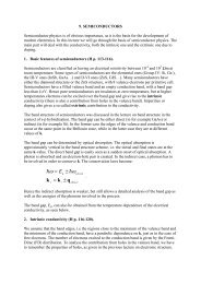
1. Introduction
Semiconductors are a group of materials, which have conductivities between those of insulators
and metals. The resistivity of a semiconductor has strong temperature dependence. You can
change the electrical conductivity of a semiconductor by introducing a controlled concentration
of impurities into the material, and this is called doping. If, for example, a silicon crystal is
doped with phosphorus, four of the five valence electrons of phosphorus will form covalent
bonds with surrounding silicon atoms. The remaining valence electron will be weakly bound to
the phosphorus atom and if the electron is excited by adding some energy, it becomes free and
will be donated to the conduction band. The silicon crystal then becomes n-doped. The crystal
may also be p-doped and it is done with atoms that will give free holes. The most common
semiconductor materials are silicon (Si), germanium (Ge) and (gallium arsenide) GaAs.
In this experiment, some groups will examine n-doped Ge. Other groups will examine Tedoped
InSb. Hall Effect measurements will be used to determine the doping concentration. The
bandgap of the examined semiconductor, the Hall coefficient, and the electron mobility will also
be determined.
2. Theory
To analyze charge transport in semiconductors, the Hall Effect (Hofmann p. 75-76) can be used.
The resistivity and the Hall coefficient, R H , are measured as a function of the temperature.
From this, the charge carrier concentration and the charge carrier mobility can be determined.
If a conductor is subjected to a current I and a magnetic field B � that are perpendicular to each
other, a potential difference occurs across the conductor in a direction which is mutually
perpendicular to I and B � . This phenomenon is called the Hall Effect.
How does it occur?
Consider a specimen as in Fig.1. If a current I flows across the sample in the x � -direction, charge
carriers q move along the x � -direction. Here, q represents � e for electrons and � e for holes,
where e is the elementary charge. If I is in the � ˆx -direction, � e moves along the � ˆx -
direction and � e moves along the � ˆx -direction. One should be careful about � and �
directions for the different cases. In Fig. 1, in order to simplify, only the case of n-doped
materials is shown. If a magnetic field B � , which is perpendicular to I � and the surface of the
sample, is applied to the sample, the magnetic force (the Lorentz force) FB � causes a deflection of
the electrons in the - y � -direction, Fig.1b. Hence, the electrons accumulate on one side of the
sample and an excess of positive ions are present on the opposite side.
3

(a)
(b)
(c)
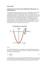
Figure1. Hall effect for an n-doped material. (a) Current flow through the specimen without magnetic
field. (b) As a magnetic field B � is applied, the electrons deflect and accumulate on one side of the
specimen. (c) The accumulated electrons give rise to an electric field y E� which causes a balance between
the electric force and the magnetic force along the y � -direction. At the newly reached balance, the
electrons flow along the x � -direction without deflecting.
4

After a short while, an electric force Fe � as a result of an electric field y E� that is caused by the
accumulation of the charges at the edges will be equal to FB � . Thus, the charges will continue to
move in the x � -direction, Fig.1c, with the drift velocity v � .
Figure 2. The Hall Effect in a semiconductor plate.
With the notation of Fig.2, we have the balance of the forces:
The relation between the magnitudes
gives
� �
F � F � 0
B e
� � �
qv �B�qE qvB � qEy
y
E � vB
y (1)
Note also that v � and y E� change direction when q changes sign. The following relation
between the current, the current density j and the drift velocity is achieved:
I � abj
(2)
5

j � ncqv (3)
UH � Eyb (4)
Here c n is charge carrier concentration (number/unit volume), H U is the Hall voltage. U H is
negative for electrons (i.e., E y is pointing to ˆy � ), and positive for holes (i.e., E y is pointing to
the � ˆy -direction).
Inserting eq. (2), (3) and (4) in (1) gives
i.e.
and the Hall coefficient is defined as:
B
abn q
n
U
b
I H
c
IB
U qa
H
� (5)
c � (6)
RH y
� E / jB
(7)
Inserting eq. (1) and (3) into (7) or inserting eq. (2) and (4) into (7) leads to the relation
R
H
U a 1
H �
IB n q
� (8)
It is seen that the sign of the Hall coefficient is given by the sign of the charge carriers or
equivalently the sign of the Hall voltage.
The conditions for the validity of the expressions above are that one type of charge carrier is
dominating and that the drift velocity is constant. If both electrons ( n ) and holes ( p ) are present
as significant charge carriers (which is often the case in semiconductors) their different mobility
( � n and � p ) must be accounted for in the expression of R H .
R H
2
p � k n
e(
kn � p)
2
c
� (9)
6

Where k � �n / � p , n is electron concentration and p is hole concentration. For strongly n -
doped or p -doped materials Eq. (9) is reduced to Eq. (8).
The sample voltage U R (see Fig.2) over the plate can be expressed as:
where the conductivity � is
c Ic
� � � � ’ (10)
URRI I
ab � ab
I c
U ab
� � . (11)
For semiconductors the conductivity may generally be expressed as
R
� � ne� � pe�
(12)
n p
In the case of dominating n -doping, we find that the mobility may be calculated by substituting
Eq. (6) and (11) in Eq. (12) as
U H c
� �
ne U RB
b
�
and analogously for � p in the case of dominating p -doping.
� n
(13)
The temperature dependence of the mobility may be expressed as
�
� � CT (14)
np ,
where � is called the temperature exponent of the mobility (C is a constant). The value of α
depends on the scattering mechanisms that influence the electron and hole mobility. When lattice
phonon scattering is dominating (i.e. at high temperature), the temperature dependence is
� �� 3/2.
When impurity scattering is dominating (i.e. at low temperature), � � 3/2.
7

3.1. Experiment: n-doped Ge
Multimeter
U H
D
I P
Carrier Board
U R
Power Supply
I P
T
HC
Multimeter
12V
AC
Phywe
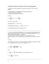
Figure 3. Experimental Setup of n-doped Ge measurements.
�
I B
DC
�
Multimeter
I B
I B
I
P
U H
U R
T
D
HC
8

1. Check the connections of the equipment according to Fig.3. Keep the sample out of the
magnet so far.
2. Measure the Hall voltage, U H , as a function of sample current I .
a) Set the display in “current” (IP) mode. ( I P denotes I on the equipment)
b) Fix the sample current as I =0 A.
c) Apply a magnetic field of 250 mT. Use the calibration table given below.
d) Check the U H value. If it is different from zero, set it to zero using the “ H U
compensate” button on the carrier board.
c) Measure U H as a function of I between -30 mA and 30 mA in steps of about 5
mA
d) Present the results in a table and a plot.
3. Measure U H as a function of B
a) Fix the magnetic field to zero.
b) Apply 30 mA sample current.
c) Check the U H value. If it is different than zero, set it to zero using the U H
d)
compensate button on the carrier board.
Change the magnetic field between 0 and 300 mT in steps according to the
calibration table. Measure U H .
e) Return the magnetic field to zero.
f) Change the polarity of the coil-current.
g) Check the H U value when the magnetic field is zero. If U H is different than zero,
set it to zero using the U H compensate button on the carrier board.
h) Change the magnetic field between 0 and -300 mT in steps according to the
calibration table. Measure U H .
i) Present the results in a table and a plot.
4. Measure H U and U R as a function of temperature.
a) Change back the polarity of the coil-current.
b) Apply 30 mA sample current.
c) Check the U H value. If it is different than zero, set it to zero using the U H
d)
compensate button on the carrier board.
Set the magnetic field to 300 mT.
e) Start the measurements by activating the heater and measure up to a maximum
temperature of 170°C. Measure H U and U R for every 5 degree.
f) Present the results in a table and a plot.
9

Sample dimensions:
a = 1 mm
b = 10 mm
c = 20 mm
Calibration Table for n‐doped Ge‐setup
B(mT) I(mA)
300 1131
270 1020
250 947
230 872
200 768
170 655
150 582
130 499
100 403
70 290
50 208
30 135
0 0
‐30 ‐79
‐50 ‐162
‐70 ‐233
‐100 ‐346
‐130 ‐460
‐150 ‐528
‐170 ‐603
‐200 ‐713
‐230 ‐825
‐250 ‐903
‐270 ‐985
‐300 ‐1114
10

3.2. Experimental Setup of Te-doped InSb
M
P
LN2
p
G
I B
I
U H
U R
UT
s
B �
U
U
U
Philips
I B
� �
H
R
T
M
B �
Figure 4. Experimental Setup of Te-doped InSb measurement.
S
P
HP
I
� �
M
G
11

On the Hall plate, thin wires are soldered, allowing H U and U R to be measured when a current
I passes through the plate, see Fig. 5. To protect the Hall plate and the wires while cooling, the
plate is mounted inside a sample holder of brass. Be very careful with the sample holder, do not
drop, hit or handle it carelessly! The thin wires are connected to cables exiting on the top of the
sample holder. These cables have different colors and Fig. 4 shows how to measure on the Hall
plate. The sample holder should not be opened because it has to be nitrogen tight. On the Hall
plate, a thermocouple is mounted (see Fig. 5) which has its reference point outside the sample
holder, placed in ice water. A calibration table is given below, to convert voltage in mV to
degrees Celsius.
white
blue green yellow
red
Figure 5. The Hall plate of Te-doped InSb and connections for H U , U R and I .
1. Check the connections according to Fig.4 and Fig.5.
black
thermocouple
2. Place the reference soldering from the thermocouple in ice water and check the temperature.
3. Cool down by slowly lowering the sample holder into the Dewar filled with liquid nitrogen,
while at the same time noting the thermo voltage, (thermocouple). Wait until the lowest
temperature possible is reached. Prepare a table of U R , and U H , measured at various U T
ranges from the lowest temperature to room temperature in steps of 0.1 mV. In the
beginning of the measurement, the temperature will increase rapidly. Therefore, prepare the
table before you start the measurement.
12

4. When it reachs the lowest temperature ( U T ~ -5.1 mV), apply a sample current of ≈ 20 mA,
which should be kept as constant as possible during the experiment. If it changes, note the
new values continuously.
5. Switch on the magnet current ≈ 2 A. This gives a magnetic field of 1000 Gauss at the
position where the sample is placed.
6. Take out the sample holder from the Dewar. Place it between the poles of the
electromagnets. The Hall plate should be perpendicular to the magnetic field and
centered between the electromagnets. The sample holder has marks indicating the
orientation of the Hall plate.
7. Take the first measuring point of U H , R U , I and U T at the possible lowest temperature.
Then, continue to take data points at every 0.1 mV up to room temperature.
8. After reaching the room temperature, turn off the magnetic field and measure U H and U R .
Ideally, H U should be zero if there is no magnetic field. But since the solder points for H U
might not be exactly perpendicular to the current path, U H is often non-zero. Correct the
data that you obtained during the measurement, with the following formula:
U ( B�0)
U () T �U () T � U () T
H H, meas
H
UR( B�0)
R
13

Sample dimensions:
a = 1 mm b = 10 mm c = 20 mm
Calibration table to convert voltage in mV to degrees Celsius:
14

4. Report Writing
The full report should include the items below, as well as background information, theory,
experimental information, results and conclusions (see the report template).
1. In appendix
Table of the measured values;
Table of the calculated values ( n c ,� , � ).
2. In Theory section, a thorough derivation of how the bandgap and the doping
concentration were determined.
3. In Result section, plots showing
ln( � ) as a function of 1/T
ln( n c ) as a function of 1/T
ln( � ) as a function of ln( T )
4. Present the experimental value of the bandgap and compare to a theoretical value
(Physics handbook or Hofmann).
5. Present the experimental value of the doping concentration.
6. Determine the Hall coefficient R H as a function of T and show in a plot.
7. Determine the temperature coefficient � from the plot ln( � ) vs. ln( T )
.
Compare with a
theoretical value.
8. In discussion, discuss the physical reasons why silicon and for example not InSb, has
been the dominating semiconductor material for electronic components.
A complement to Hofmann chap. 7 is available as an appendix from B.G. Streetmans book
"Solid State Electronic Devices" (Prentice-Hall 1980) chap. 3.3.3 and 3.4.2.
15