Problem Set 1

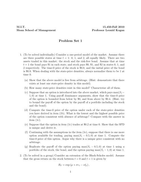
M.I.T. 15.450-Fall 2010
Sloan School of Management
Professor Leonid Kogan
Problem Set 1
1. (To be solved individually) Consider a one-period model of the market. Assume there
are three possible states at time t = 1: 0, 1, and 2, all equally likely. There are two
assets traded in this market: the stock and the risk-free bond. Assume that at time
t = 1 the bond pays $1 in each state, and stock pays $0, $1, and $2 in states 0, 1, and
2 respectively. The time-0 price of the stock is $0.8, and the initial price of the bond
is $0.9. When dealing with the state-price densities, always normalize them to be 1 at
time 0.
(a) Show that the above model is free from arbitrage. (Hint: demonstrate that there
exists at least one state-price density in this model).
(b) How many state-price densities exist in this model? Characterize all of them.
(c) Suppose that an option is introduced into the above market, which pays max(S 1 −
1, 0) at time 1. Using payoff dominance arguments, show that the time-0 price
of the option is bounded from below by $0, and from above by $0.4. (Hint: try
to bound the payoff of the option by the payoff of a portfolio including the stock
and the bond).
(d) Compute the time-0 price of the option under each of the state-price densities
you have derived in item (1b). What is the lowest and the highest possible price
of the option consistent with absence of arbitrage? Compare with the answer in
item (1c).
(e) Suppose that the option in item (1c) trades at $0.2 at time 0. Show that the SPD
is unique and derive it.
(f) Continuing with the assumptions in the item (1e), suppose that there is one more
option available for trading, paying max(S 1 − 0.5, 0) at time 1. Compute the
time-0 price of this option. Argue why there is a unique price consistent with no
arbitrage.
(g) Replicate the payoff of the option paying max(S 1 − 0.5, 0) at time 1 using a
portfolio of the stock, the bond, and the option paying max(S 1 − 1, 0) at time 1.
2. (To be solved in a group) Consider an extension of the Black-Scholes model. Assume
that the gross return on the stock between t = 0 and t = 1 is given by
R T = exp (µ + σε 1 − νξ 1 ) ,
1

where ε 1 and ξ 1 are independent. Assume that ε 1 ∼ N (0, 1), while ξ 1 is exponentially
distributed: for any a, Prob(ξ 1 > a) = exp(−a). Assume that ν > 0. Assume that the
gross return on the risk-free bond between 0 and 1 is given by exp(r).
The above model adds a single negative jump to the Black-Scholes setting. ν parameterizes
the distribution of the jump.
Assume the following parameter values:
r = 0.05, σ = 0.2, ν = 0.05.
Assume that under the risk-neutral probability, the jump remains exponentially distributed:
the risk-neutral distribution of ξ 1 is the same as physical, while the riskneutral
jump distribution parameter is ν Q = 0.2. Moreover, assume that the riskneutral
distribution of ε 1 is normal with variance 1 and mean −η, η = 0.25.
(a) Compute µ (Hint: you may want to look up the moment-generating function for
an exponential random variable).
(b) Assume that the initial stock price is S 0 = 1. Consider European put options
maturing at T = 1 with strike prices K = 0.5, 0.6, ..., 1, ..., 1.5. Compute the
Black-Scholes implied volatilities for these put options and plot them as a function
of the strike price. (Hint: Conditional on ξ 1 , stock return distribution is
lognormal, like in the Black-Scholes model). Compute the absolute value of the
Sharpe ratio of returns on each put option. Repeat this exercise for ν Q = 0.05.
Comment on the differences in results.
3. (To be solved individually) Consider a zero-coupon corporate bond maturing at time
t = 1, with the face value of $1. Assume that the state of the firm is captured by
the random variable X 1 . The bond defaults if X 1 ≤ A, in which case it pays nothing.
Assume that X 1 ∼ N (0, 1). Let the state-price density be given by
π 1 = exp −r f − η 2 /2 − ηY 1 , π 0 = 1
where Y 1 ∼ N (0, 1). Assume that corr(X 1 , Y 1 ) = ρ. (Hint: Y 1 can be written as
ρ X 1 + (1 − ρ 2 ) Z 1 where X 1 and Z 1 are independent).
You are supposed to perform the following analysis analytically. To help your intuition,
you may want to perform numerical calculations first by assuming specific parameter
values.
(a) Derive the default probability p def .
(b) Derive the price of the bond at time t = 0. (Hint: It is simpler to perform
calculations under the risk-neutral probability measure).
(c) Derive the bond yield and the Sharpe ratio of bond returns. Relate both to ρ, η,
p def , and comment on the relationship.
2

(d) This question is relatively open-ended. A qualitative answer would be acceptable.
How would you build a model of corporate bond prices, so that bond yields
change significantly over time (e.g., widen in times of economic distress), while
the likelihood of default changes much less?
3

MIT OpenCourseWare
http://ocw.mit.edu
15.450 Analytics of Finance
Fall 2010
For information about citing these materials or our Terms of Use, visit: http://ocw.mit.edu/terms.