AIR POLLUTION – MONITORING MODELLING AND HEALTH

31.08.2015 Views
288 Air Pollution – Monitoring, Modelling and Health spline (Chapra & Canale, 1987; Samoli et al., 2011; Schwartz et al., 1996), the other ones are usually applied in GAM. Using splines, polynomial functions will be provided for each defined interval instead of a single polynomial for the whole database. The natural cubic spline is based on third order polynomials derived for each interval between two knots at fixed locations throughout the range of the data (Chapra & Canale, 1987; Peng et al., 2006). The choice of knots locations can result in substantial effect on the resulting smooth. So, in Peng et al. (2006) study the authors “provided a comprehensive characterization of model choice and model uncertainty in time series studies of air pollution and mortality, focusing on confounding factors adjustment for seasonal and long-term trends”. According to their results, for natural splines, the bias drops suddenly between one and four degrees of freedom (df) per year and is stable afterwards, suggesting that at least 4 degrees of freedom per year of data should be used. In such way, in time series studies of air pollution and mortality (or morbidity) usually is used four to six knots per year, as the seasonality trend is due to the different behavior of variables during the seasons of the year (Tadano, 2007). Their results show that “both fully parametric and nonparametric methods perform well, with neither preferred. A sensitivity analysis from the simulation study indicates that neither the natural spline nor the penalized spline approach produces any systematic bias in the estimates of the logrelative-rate ” (Peng et al., 2006). The smooth functions of time accounts only for potential confounding factors which vary smoothly with time, such as seasonality. Some potential confounders which vary on shorter timescales are also important, as they confound the relationship between air pollution and health outcomes, such as day of the week and holiday indicator (Peng et al., 2006). 4.2.2 Day of the week and holiday indicator Important potential confounding factors that may bias time series studies of air pollution and mortality (or morbidity) are factors which vary on shorter timescales like calendar specific days, such as day of the week and holiday indicator (Lipfert, 1993). These trends are not necessarily present, but they occur often enough that they should be checked (Samoli et al., 2011; Schwartz et al., 1996). For example, on weekends the number of hospital admissions can be lower than on weekdays and can also be lower during holidays. One way to adjust according the week day trend is to add qualitative explanatory variable for each day of the week (varying from one to seven) starting at Sundays. To adjust the holiday indicator, it can be considered an additional binomial explanatory variable in which one means holidays and zero means workdays (Tadano et al., 2009). Adding all the time trends mentioned and explanatory variables in the GLM with Poisson regression, the expression used in some studies of air pollution impact on population’s health is as follows (Tadano, 2007): 0 1 2 3 4 5 6 ln y T RH PC H dow ns, (6) where y = health outcome of interest; T = air temperature or dewpoint temperature (ºC); RH = air relative humidity (%); PC = pollutant concentration (g/m 3 ); H = time trend

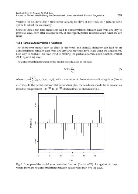
Methodology to Assess Air Pollution Impact on Human Health Using the Generalized Linear Model with Poisson Regression 289 variable for holidays; dow = time trend variable for days of the week; ns = natural cubic spline to adjust for seasonality. Some of these short-term trends can lead to autocorrelation between data from one day to previous days, even after its adjustment. In this regard, partial autocorrelation functions are used. 4.2.3 Partial autocorrelation functions The short-term trends such as days of the week and holiday indicator can lead to an autocorrelation between data from one day and previous days, even using the adjustment. One way to analyze this time trend is plotting the partial autocorrelation function (Partial ACF) against lag days. The autocorrelation function of the model’s residuals is as follows: 1 n k where ck yi yik c k c0 ACF , (7) , with n = number of observations and k = lag days (Box et n i1 al., 1994). In the partial autocorrelation function plot, the residuals should be as smaller as possible, ranging from 2n 12 12 to 2n (dashed lines) as shown in Fig. 1. Partial ACF -0.05 0.00 0.05 0 5 10 15 20 25 Fig. 1. Example of the partial autocorrelation function (Partial ACF) plot against lag days where there are no autocorrelations between data for less than five lag days. Lag

Page 1 and 2: AIR POLLUTION - MONITORING, MODELLI

Page 5 and 6: Contents Preface IX Chapter 1 Urban

Page 9: Preface This book provides a compre

Page 12 and 13: 2 Air Pollution - Monitoring, Model




Page 20 and 21: 10 Air Pollution - Monitoring, Mode













































Page 110 and 111: 100 Air Pollution - Monitoring, Mod














































































































































Page 396: 386 Air Pollution - Monitoring, Mod

pollution

monitoring

concentration

emissions

particles

concentrations

exposure

urban

studies

atmospheric

modelling

ademloos.be

AIR POLLUTION – MONITORING MODELLING AND HEALTH

air pollution â monitoring, modelling and health - Ademloos ... View more air pollution â monitoring, modelling and health - Ademloos

Delete template?

Save as template ?

air pollution â monitoring, modelling and health - Ademloos air pollution â monitoring, modelling and health - Ademloos