Quantifying tail dependency - Barrie & Hibbert

Risk aggregation: generalising dependency 

Relationships in the Barrie & Hibbert ESG 

Steven Morrison PhD 

September 2010 

01 

Global insurance risk management report 

www.barrhibb.com Page

Contents 

Introduction ...................................................................................................... 3 

Dependency in the Barrie & Hibbert ESG ................................................................... 4 

Alternative shock distribution choices ....................................................................... 6 

Quantifying tail dependency .................................................................................. 7 

1-year VaR case study .......................................................................................... 9 

Single-factor models for interest rates and equity returns ........................................ 9 

Multi-factor models for interest rates and equity returns ........................................ 12 

Summary ......................................................................................................... 16 

www.barrhibb.com Page 2

Introduction 

The use of 1-year Value-at-Risk (VaR) in insurance groups’ principle-based capital assessment has become 

increasingly common in recent years, both for group-wide Economic Capital purposes and in regulatory 

capital assessments such as Solvency II’s Solvency Capital Requirement (SCR). 1-year VaR capital 

assessments depend critically on the assumed joint distribution of all risk factors affecting the balance sheet at 

a 1-year time horizon, or, in other words, how the different sources of risk are aggregated. 

When thinking about the joint distribution of a number of risk factors, it can be convenient to separate out the 

distribution into two distinct components: 

1. The marginal distributions of each individual risk factor. 

2. The copula, which is a description of the dependency between risk factors. 

Thinking of the distribution in this way, we can consider the effect of changing one of the individual 

components while leaving the others unchanged. In particular, we can consider changing the dependency 

structure through different choices of copula and examine the effect on model results (for example the SCR). 

In recent years this separation of marginal distributions and copula has provided a useful tool in educating 

modellers about dependency, in particular that there is more to dependency than ‘just’ correlation. This has 

highlighted the concept of ‘tail dependency’, which refers to the tendency for different risk factors to 

simultaneously take extreme values. Furthermore, we usually have more confidence in our view of individual 

marginal distributions than on the dependency structure, so may be interested in stressing these dependency 

assumptions while keeping marginal distributions fixed. 

In this note, we describe how dependency arises in the ESG and how we can change dependency through 

changing the distribution of the random shocks used to drive the ESG models. We then demonstrate the 

effect of changing dependency in this way using a simple 1-year VaR case study. 


Dependency in the Barrie & Hibbert ESG 

First, let’s clarify how dependency between risk factors arises in the Barrie & Hibbert ESG. 

Barrie & Hibbert’s ESG is a multi-period, structural model. It is multi-period in the sense that it describes the 

path of risk factors at multiple points in time and not just their values at a single point in time. In fact, most of 

the models adopted by Barrie & Hibbert are fundamentally continuous-time models, i.e. they describe the 

entire continuous path of risk factors, though in practice the models need to be implemented in such a way 

that the path is sampled at discrete (e.g. monthly or annual) time steps. 

It is also a structural model, in the sense that different risk factors are connected via specified structural 

relationships. To give a simple example, equity total returns are constructed by adding an excess return onto 

the risk-free short-term interest rate, so that when risk-free interest rates are relatively large (small) we 

expect, on average, that the total nominal returns of risky assets’ will also be relatively large (small). The use 

of a multi-period model also builds in certain structural relationships over time, such as mean-reversion of 

interest-rates, i.e. when interest rates are relatively large (small) relative to their average levels we expect, on 

average, that they will decrease (increase). So dependency between risk factors at any given time horizon 

comes about partly because of the assumed structural relationships between them and the assumed 

structural relationships over time. 

Exhibit 1 indicates the main structural relationships between risk factors in Barrie & Hibbert’s ESG. 

Exhibit 1 

Overview of Barrie & Hibbert’s ESG structure 


The green boxes in Exhibit 1 indicate stochastic models for individual risk factors. Within each of these 

models, stochastic changes in risk factors (over a model time step, such as one month or one year) arise due 

to random ‘shocks’, sampled using a random number generator. Furthermore, the shocks to different risk 

factors are, in general, dependent. They are sampled from some joint distribution, with a dependency 

structure. So dependency between risk factors also arises due to the assumed dependency between shocks. 

In summary, dependency between risk factors at any given time horizon arises through a combination of: 

1. The assumed model structure. 

2. The assumed joint distribution of the shocks. 

If we want to change the dependency between risk factors, we can do so either by changing model structure, 

or the joint distribution of the shocks, or a combination of the two. 

Changing the dependency structure through choice of model structure is attractive, since it helps us to 

explain dependency in fundamental terms. As noted above, we usually have little confidence in dependency 

relationships based on analysis of historical data alone, largely because there are so few historical 

observations to base such an analysis on. Imposing structure on the model naturally ‘shapes’ the dependency 

structure in a way that reflects our fundamental economic views. 

Furthermore, model structure allows us to capture fundamental relationships between dependency and 

marginal distributions. Though it can be convenient to think about dependency separately from marginal 

distributions, this doesn’t reflect the fact that both are driven by the same fundamental economic drivers. For 

example, it seems natural that correlation between different equity markets increases at times of high 

volatility in all individual markets. The fundamental economic driver here is the volatility of the global 

influences of equity market returns, and this affects both the marginal distribution of individual markets and 

their dependency at the same time. It turns out that this feature can be built into the model structure relatively 

easily, and Barrie & Hibbert provide a model that does this – the SVJD model. So, in this case the user can 

change dependency via changing model structure, though the choice of structure also means that the 

marginal distributions change (naturally) at the same time. 

We believe that coherent economic structure has a crucial role to play in rigorous multi-asset real-world 

modelling. However, making fundamental changes to model structure can be a significant task. It may also be 

useful to have some flexibility to make quicker changes to dependency relationships in the model, for 

example, for the purposes of testing capital assessment results’ sensitivities to dependency relationships 

where we may not have strong views on model structure to help guide these assumptions. Interest in such 

functionality could arise from a firm’s consideration of the model risk in their Internal Model, or from specific 

requests arising from their regulator’s review of their Internal Model implementation. The alternative method 

of changing dependency by changing the joint distribution of shocks provides such an approach, and can be 

implemented easily using the Barrie & Hibbert ESG’s Shock Import functionality 1 . 

1 See ESG help for details on how to do this. 


Alternative shock distribution choices 

Using the Shock Import functionality, the user can import any shocks of their choosing. In this note we will 

focus on shocks generated from a particular class of distributions – the joint distribution having standard 

normal marginal distributions and a t copula. 

As described in the introduction, a general multivariate distribution can be described in terms of its individual 

marginal distributions along with its copula, which separately describes its dependency. Such a separation 

allows one to construct ‘meta-distributions’ by combining different copulas and marginal distributions. For 

example, one could construct a bivariate distribution where one variable has a uniform distribution, the other 

has a normal distribution and the copula is that of a t distribution with 5 degrees of freedom. 

Here we will consider shocks generated from the class of meta-distributions having standard normal marginal 

distributions but with different t copulas. This means that the marginal distributions of shocks are unchanged 

from those assumed in the ESG’s internal random number generator, but the dependency structure is more 

general. By retaining the same marginal distributions the intention is to have minimal impact on the resulting 

marginal distributions of the risk factors. It should be noted that in practice, depending on the ESG model 

structure chosen, changing the shock copula may have some effect on the marginal distributions of risk 

factors (even if the marginal distributions of the shocks are unchanged). This is discussed further in the case 

study below. 

The choice of the t copula is by no means the most general assumption we can make. However, it is a natural 

generalisation of the Gauss copula (the copula assumed in the ESG’s internal random number generator). 

Like the Gauss copula, it is parameterised by a correlation matrix specifying the ‘overall level’ of correlation 

between risk factors. However, we now have a single additional parameter – the ‘number of degrees of 

freedom’ of the corresponding t distribution, with the Gauss copula being the limiting case as the number of 

degrees of freedom tends to ∞. This additional degree of freedom allows us to control the level of ‘tail 

dependency’ - the tendency for different risk factors to simultaneously take extreme values. 


Quantifying tail dependency 

Dependency can be described in many ways. There are a number of correlation coefficients describing the 

overall level of dependency, and a number of measures of tail dependency, which measure the level of 

dependency at the extremes of the distribution. Though such statistics do not tell us everything about the 

dependency structure, they summarise some of the key features of dependency and allow us to compare 

different joint distributions in relatively simple terms. Here we will quantify tail dependency as follows. 

Firstly, we define the Probability of Joint Quantile Exceedance, at various probability levels. For a given 

probability level, this measures the probability that both risk factors simultaneously exceed that probability 

level. Mathematically: 

where is the probability level and are cumulative probability distributions for the marginal 

distributions of the two risk factors . 

We then define the Conditional Probability of Joint Quantile Exceedance as the conditional probability of one 

risk factor exceeding each probability level, given that the other risk factor exceeds that level. 

Mathematically: 

Note that we have defined these statistics in terms of the left hand tail of each of the marginal distributions, 

but similar statistics can be defined for the other ‘quadrants’ of the joint distribution. 

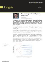
The calculation of these statistics is indicated in Exhibit 3, which shows 10,000 samples from three different 

copulas – the Gauss, t5 and t2 copulas 2 . In all cases the marginal distributions are standard normal and the 

linear correlation is approximately +0.5 3 . The red lines indicate quantiles at the p=1% level. The JPQE 

measures the proportion of samples which lie in the area below the dashed red line and to the left of the solid 

red line, while the CPJQE measures this number as a proportion of the samples to the left of the solid red line. 

Note that the CPJQE at the 1% level is 12.9% for the Gauss, 25.9% for the t5 copula and 39.5% for the t2 

copula (despite the fact that the overall level of correlation is the same in both cases), indicating a stronger 

level of tail dependency as we decrease the number of degrees of freedom for the t copula. 

Exhibit 3 

10,000 pairs of shocks with standard normal marginal distributions, correlation = 0.5 but different copulas 

2 Here we refer to the copula of the t distribution with 5 degrees of freedom as the t5 copula, and the copula of the t 

distribution with 2 degrees of freedom as the t2 copula. 

3 Strictly speaking, the rank correlation is exactly the same in all cases, but there are small differences in the linear 

correlation. 


Exhibit 4 further illustrates the difference in tail dependency for different copulas, showing the CPJQE at 

different probability levels from 1% to 10%. This shows not just the differences at different fixed probability 

levels, but also indicates how the CPJQE changes with a decrease in the probability level i.e. as we go further 

into the tail. In fact, for the Gauss copula, the CPJQE tends to zero in the limit as the probability level tends to 

zero, while for the t copulas this limiting CPJQE is non-zero (20.7% for the t5 copula for this level of 

correlation) 4 . 

Exhibit 4 

Tail dependency for three different choices of copula (correlation = 0.5) 

Conditional Probability of Joint Quantile 

Exceedence 

40% 

35% 

30% 

25% 

20% 

15% 

10% 

5% 

0% 

4 This limiting statistic is a popular measure of tail dependency, sometimes known as the ‘coefficient of (lower) tail 

dependence’. 

0% 1% 2% 3% 4% 5% 6% 7% 8% 9% 10% 

Probability level 

t5 Copula 

Gauss Copula 


1-year VaR case study 

To illustrate the effect of changing the shock copula, we will calculate the 1-year VaR for a straightforward 

asset-liability position: we will define the liability as a vanilla 10-year put option on an equity total return 

index, struck at the forward price; and assume that the assets backing this liability are invested in cash. 

In this case, the value of the asset-liability position in one year depends on the end-year values of three key 

risk factors: the equity total return index, the 9-year risk-free rate, and the 9-year equity implied volatility. For 

simplicity we will assume a fixed implied volatility 5 of 20% and generate scenarios for the other two risk 

factors using the Barrie & Hibbert ESG under real-world calibration assumptions. 

Barrie & Hibbert’s ESG provides a flexible modelling framework with a number of different model choices 

and calibrations for each risk factor. For the specific purpose of 1-year real-world projection, Barrie & 

Hibbert’s recommended ESG configuration adopts ‘multi-factor’ models for both interest rates and equity 

returns. By ‘multi-factor’ here, we mean that changes in each individual risk factor are generated using a 

number of shocks. Our recommended real-world interest rate model, the 2-factor Black-Karasinksi model, is a 

model in which interest rate changes are driven by two shocks, while our recommended equity model is a 

model in which equity returns on each individual market are generated by at least 7 shocks (6 ‘systematic’ 

shocks, which are common to all equity markets, and a single ‘idiosyncratic’ shock per market) 6 . The use of a 

multi-factor interest rate model means that different points on the yield curve are less than perfectly 

correlated, while the use of a multi-factor equity model provides a convenient way of describing correlation 

across numerous equity markets, as well as providing a natural mechanism for generating elevated tail 

dependency between equity markets (if the SJVJD model is used). So this model structure, in which both 

interest rates and equity returns are generated using numerous underlying shocks, has been chosen 

deliberately to give certain realistic market features that can be important for 1-year real-world projection. 

However, a potential drawback of such a multi-factor approach is that there is a relatively complicated 

relationship between the joint distribution of risk factors and that of the shocks. In such a model, changing 

the distribution of the shocks (either by changing their marginal distributions or their copula), has a complex 

effect on the distribution of the risk factors that are derived from them. For example, changing the shock 

copula changes the marginal distribution of the risk factors even if the marginal distribution of the shocks is 

unchanged. In order to clarify this, and other related effects, below we will also consider a simpler Barrie & 

Hibbert ESG model structure in which each individual risk factor is generated using a single shock (hence a 

‘single-factor’ model). The price that one pays for such a simpler model is that (depending on the exact 

requirements of the model) it is potentially less realistic than the multi-factor model. However, it can provide 

some useful insights before moving on to the more complex, and realistic, multi-factor model. 

Of course, in considering different choices of copula between equity returns and interest rates, this naturally 

leads us to the question of which is the ‘right’ one. Empirical data analysis will only be able to take us so far 

here – there is unlikely to be sufficient historical annual data to allow many meaningful statements about the 

precise statistical nature of this tail dependency. However, this highlights the advantage of this flexible, fast 

approach to stress testing the copula assumption. 

Single-factor models for interest rates and equity returns 

Firstly, we consider the following single-factor models: 

Interest rates: 1-factor Libor Market Model. 

Equities: 1-factor constant volatility model 7 . 

Barrie & Hibbert don’t provide a standard real-world calibration of this model configuration, but we have 

prepared a calibration to be broadly consistent with our standard real-world calibrations of our recommended 

(multi-factor) models at end-December 2009. 

Note that for the purpose of illustration in this particular case study, since capital requirements increase when 

both equities and interest rates fall, we have chosen a (small) positive correlation between equity returns and 

5 Note that B&H ESG 7 does provide a stochastic equity option-implied volatility model but we have chosen to keep this 

risk factor fixed in this analysis as a two-dimensional case study is simpler than a three-dimensional one! 

6 In fact, further additional shocks are required if a Stochastic Volatility Jump Diffusion model is used. 

7 In the ESG, this is set up using the ‘ParentEquityAssetCorrelationModel’, which is our recommended method for 

modelling equities for market-consistent applications. 


interest rate changes. Our standard real-world calibrations actually assume a small negative correlation here, 

which is consistent with long-term ‘through the cycle’ (TTC) correlation behaviour, though recent historical 

data indicates that it would be reasonable to assume a positive correlation on a ‘point in time’ (PIT) basis. 

For our case study, we have generated two sets of 100,000 scenarios under two different copula 

assumptions: the Gauss copula (generated using the ESG’s internal random number generator) and the t5 

copula (generated externally and imported using the shock import functionality). Apart from the different 

choices of copulas for the shocks, all other model and calibration assumptions are the same in both cases. In 

particular both the equity shock and the interest rate shock have standard normal marginal distributions and 

we assume the same rank correlation between them. 

Firstly we check the effect of changing the shock copula on the marginal distributions of our risk factors. Due 

to the simple one-to-one relationship between risk factors and shocks, the marginal distributions of each of 

the risk factors should be unchanged if the marginal distributions of the shocks are unchanged. 

To check this, we have measured the marginal distributions of our two risk factors – the equity return over 

the year, and the 9-year spot rate at the end of the year – using 100,000 scenarios. Exhibits 5 and 6 show the 

left-hand tail of the distributions of the equity log-return and 9-year spot rate respectively. Both probability 

distributions are shown in cumulative terms. As expected, we have been able to change the copula 

relationship between the random shocks driving the ESG without changing the marginal distributions of the 

risk factors. 

Exhibit 5 

Comparison of marginal distributions of equity return under different shock copulas (‘single-factor’ models) 

t5 Shock Copula 

Gauss Shock Copula 

-45% -35% -25% -15% 

Exhibit 6 

Comparison of marginal distributions of 9-year spot rate under different shock copulas (‘single-factor’ models) 


Equity return 


2.5% 3.0% 3.5% 4.0% 

9-year spot rate 

www.barrhibb.com Page 10 

10% 

9% 

8% 

7% 

6% 

5% 

4% 

3% 

2% 

1% 

0% 

10% 

9% 

8% 

7% 

6% 

5% 

4% 

3% 

2% 

1% 

0% 

Cumulative Probability 

Cumulative Probability

Changing the shock copula doesn’t change the marginal distributions of risk factors, but should change the 

level of tail dependency between risk factors. To demonstrate this, Exhibit 7 compares tail dependency 

statistics for the two choices of shock copula. Tail dependency is quantified using the Conditional Probability 

of Joint Quantile Exceedance. We estimate these statistics empirically using the 100,000 scenarios generated 

under our two different shock copula assumptions. 

As expected, moving from a Gauss to a t5 copula increases the tail dependency between the shocks, and this 

gives rise to increased tail dependency between the risk factors derived from these shocks. 

Furthermore in this case, due to the simple one-to-one relationship between risk factors and shocks, we 

expect the copula between the risk factors to be exactly the same as the copula between the shocks. As a 

simple check of this, we have also calculated our tail dependency statistics under ‘equivalent’ Gauss and t5 

copulas. By ‘equivalent’ we mean that these copulas have the same overall level of correlation 8 . Though these 

tail dependency statistics don’t tell us everything about dependency, these results indicate that the 

dependency between risk factors looks like a Gauss copula if the underlying shocks are generated using a 

Gauss copula, and looks like a t5 copula if the shocks are generated using a t5 copula. Thus we have direct 

control over the copula between risk factors via our choice of shock copula, and the tail dependencies can be 

changed without impacting on the marginal distributions. 

Exhibit 7 

Tail dependency between risk factors under two different choices of shock copula (‘single-factor’ models) 


Exceedence 


Exceedence 

20% 

18% 

16% 

14% 

12% 

10% 

8% 

6% 

4% 

2% 

0% 

20% 

18% 

16% 

14% 

12% 

10% 

8% 

6% 

4% 

2% 

0% 


0% 1% 2% 3% 4% 5% 6% 7% 8% 9% 10% 



0% 1% 2% 3% 4% 5% 6% 7% 8% 9% 10% 


B&H ESG 

Equivalent t5 

Copula 

Equivalent Gauss 

Copula 

B&H ESG 

Equivalent t5 

Copula 


Copula 

8 Here we measure ‘overall’ correlation using Kendall’s tau rank correlation measure. 


Finally, we examine the effect of the copula assumptions on the 1-year VaR for our case study –a liability of a 

10-year put option on an equity fund of £1m, struck at the forward price and with backing assets invested 

wholly in cash. We assume that the equity implied volatility is fixed at 20%. At end-December 2009 (using the 

Government yield curve) this implies an initial liability value of £0.248m. 

Exhibit 8 shows the tail of the distribution of the capital requirement under the two different choices of shock 

copula. In particular, the 99.5% VaR (in excess of the time-0 liability value) is £0.261m and £0.278m under 

Gauss and t5 shock copulas respectively. Unsurprisingly, the VaR capital requirement increases as we move 

from the Gauss to t5 copula – the capital requirement is driven by exposures to falls in equity values and falls 

in interest rates; assuming that these jointly occur with greater joint ‘severity’ fattens the tail of the distribution 

of possible capital requirements, and hence increases the capital assessment. Put another way, the move 

from the Gauss to t5 copula has reduced the diversification credit produced in the capital assessment. The 

stand-alone equity and interest rate VaR requirements are £0.211m and £0.083m respectively 9 . So moving 

from a Gauss to t5 copula has roughly halved the diversification benefit, from £0.034m to £0.016m. 

Exhibit 8 

Distribution of capital requirement under different shock copulas (‘single-factor’ models) 

Probability Level 

100.0% 

99.9% 

99.8% 

99.7% 

99.6% 

99.5% 

99.4% 

99.3% 

99.2% 

99.1% 

99.0% 

98.9% 

Multi-factor models for interest rates and equity returns 

In the models considered so far there is a simple one-to-one relationship between risk factors and shocks. As 

we have seen, this allows us to change the copula between risk factors without changing their marginal 

distributions and allows us direct control over the type of copula between risk factors. 

Now we will consider a more complex multi-factor model, consisting of the following components: 

Interest rates: 2-factor Black-Karasinski model 

Equities: 6-factor equity model with Stochastic Volatility Jump Diffusion (SVJD) 

This is Barrie & Hibbert’s standard recommended ESG configuration for 1-year real-world modelling. Here we 

have used Barrie & Hibbert’s standard multi-year real-world calibrations of these models at end-2009 but, as 

above, flipped the sign of the equity vs rate correlation for the purpose of illustration in this particular case 

study. 

As before, we have generated two sets of 100,000 scenarios under two different copula assumptions: the 

Gauss copula (generated using the ESG’s internal random number generator) and the t5 copula (generated 

externally and imported using the shock import functionality). Apart from the different choices of copulas for 

the shocks, all other model and calibration assumptions are the same in both cases. In particular all shocks 

have standard normal marginal distributions and the same rank correlation parameters are assumed. 

9 These ‘stand-alone’ capital requirements are calculated by setting one risk factor to its 99.5% level and the other to its 

forward level. 

0.20 0.25 0.30 0.35 0.40 

Capital Requirement (£m) 




Firstly we check the effect of changing the shock copula on the marginal distributions of our risk factors. 

Now, since each risk factor is dependent on a number of shocks, we might expect the marginal distribution of 

the risk factors to depend not only on the marginal distribution of the shocks, but also their dependency. So 

even though we have assumed standard normal marginal distributions for the shocks, changing their copula, 

or indeed simply changing their correlation, is expected to have some effect on the marginal distributions of 

risk factors derived from these (multiple) shocks. 

Exhibits 9 and 10 show the left-hand tail of the distributions of the equity log-return and 9-year spot rate 

respectively, under our two different assumptions for the copula between shocks. For both risk factors 

considered here, the changes in the shock copula have had a small impact on the marginal distributions of the 

risk factors: the 99.5 th percentile of the equity return is estimated as -45.4% and -46.3% for the Gauss and t5 

copulas respectively, whilst the 99.5 th percentile of the 9-year spot rate (continuously compounded) is 2.91%, 

and 2.83% for Gauss and t5 copulas respectively 10 . 

Exhibit 9 

Comparison of marginal distributions of equity return under different shock copulas (‘multi-factor’ models) 



-45% -35% -25% -15% 

Exhibit 10 

Comparison of marginal distributions of 9-year spot rate under different shock copulas (‘multi-factor’ models) 


Equity return 


2.5% 3.0% 3.5% 4.0% 

9-year spot rate 

Exhibit 11 compares tail dependency statistics for the two choices of shock copula. As before, changing the 

underlying shock copula changes the tail dependency between risk factors derived from these shocks, and 

10 Of course, all percentiles are estimated using 100,000 scenarios and so are subject to sampling error. 

www.barrhibb.com Page 13 

10% 

9% 

8% 

7% 

6% 

5% 

4% 

3% 

2% 

1% 

0% 

10% 

9% 

8% 

7% 

6% 

5% 

4% 

3% 

2% 

1% 

0% 

Cumulative Probability 

Cumulative Probability

increasing the tail dependency of the shocks (by decreasing the number of degrees of freedom) also 

increases the tail dependency between risk factors 11 . 

However, unlike in the single-factor model case, here the copula between risk factors is, in general, different 

from the copula used to generate the shocks. Exhibit 11 illustrates the difference between the (derived) 

copula between risk factors and the assumed copula between underlying model shocks. In the special case 

where the shocks are generated using a Gauss copula, the level of tail dependency between the risk factors is 

similar to that of a Gauss copula with the same rank correlation. However, for the t5 shock copula, the copula 

between risk factors is quite different from the copula between underlying shocks. If a t5 copula is used for 

the shocks, the resulting tail dependency between risk factors is stronger than an equivalent Gauss copula, 

but not quite as strong as an equivalent t5 copula. There is some ‘dilution’ of dependency as we move from 

the model shocks to the risk factors derived from these. This comes about because of the assumed multifactor 

structure of the models. 

Exhibit 11 

Tail dependency between risk factors, compared to ‘equivalent’ Gauss and t5 copulas (‘multi-factor’ models) 


Exceedence 


Exceedence 

12% 

10% 

8% 

6% 

4% 

2% 

0% 

12% 

10% 

8% 

6% 

4% 

2% 

0% 

It is worth noting that this dilution effect, and the effect on marginal distributions, will be present to some 

degree in any model in which risk factors are built up using multiple shocks. In particular, most yield curve 

models are likely to be built using such a structure, unless interest rates of different maturities are assumed to 

be perfectly correlated. More realistic yield curve models are likely to be driven by 2 or 3 shocks (commonly 

referred to as Principal Components). So, any multi-factor interest rate model, whether an arbitrage-free 

short-rate model or a non-arbitrage free PCA model, will have this same issue: changing equity / interest rate 

11 The ‘lumpiness’ of these curves simply indicates sampling error in the estimation of CPJQEs, particularly as we go 

further into the tail. 


0% 1% 2% 3% 4% 5% 6% 7% 8% 9% 10% 



0% 1% 2% 3% 4% 5% 6% 7% 8% 9% 10% 


B&H ESG 

Equivalent t5 

Copula 


Copula 

B&H ESG 

Equivalent t5 

Copula 


Copula 


tail dependency by changing the copula relationships between the multiple factor shocks will not result in the 

same copula relationships between equities and rates. 

Nevertheless, the ability to change the shock copula gives us control over the level of tail dependency 

between risk factors, and for this particular choice of copula family, the ‘degrees of freedom’ parameter 

provides a simple dial allowing us to change the overall level of tail dependency between risk factors. 

Finally, we examine the effect of the copula assumptions on the 1-year VaR for our case study. Exhibit 12 

shows the tail of the distribution of the capital requirement under the two different choices of shock copula. 

In particular, the 99.5% VaR (in excess of the time-0 liability value) is £0.296m and £0.309m under Gauss and 

t5 shock copulas respectively. Unsurprisingly, the VaR capital requirement increases as we move from the 

Gauss to t5 copula – as in the single-factor case, joint large falls in equity prices and interest rates (which 

increase capital requirements) are more likely when we move to the t5 copula, and hence increases the 

capital assessment. In addition here the marginal distributions for both equity returns and interest rates are 

fattened as we move to the t5 copula, and this also contributes to an increased capital requirement. 

Due to these two contributing components to the increase in capital requirements – increased tail 

dependency and increased marginal tails – it is hard to quantify the effect attributable to each component 

individually. Now the stand-alone equity and interest rate VaR requirements are £0.245m and £0.091m using 

the Gauss copula but £0.251m and £0.098m using the t5 copula, so the sum of these marginal contributions 

to capital changes by roughly the same amount as the total capital requirement when we change copulas. In 

other words, the diversification benefit is similar for both choices of copula, being £0.040m under the Gauss 

copula and £0.041m under the t5 copula. This simply reflects the fact that this measure of diversification 

benefit doesn’t adequately separate out the effect of dependency alone. 

Exhibit 12 

Distribution of capital requirement under different shock copulas (‘multi-factor’ models) 

Probability Level 

100.0% 

99.9% 

99.8% 

99.7% 

99.6% 

99.5% 

99.4% 

99.3% 

99.2% 

99.1% 

99.0% 

98.9% 

0.20 0.25 0.30 0.35 0.40 

Capital Requirement (£m) 




Summary 

In this note, we have described a relatively straightforward way of changing dependency in the Barrie & 

Hibbert ESG, through changing the distribution of the random shocks used to drive the ESG models. This 

makes use of the ‘shock import’ functionality of the ESG, allowing the user to import shocks with a general 

dependency structures of their choosing. Whilst Barrie & Hibbert strongly believe in the need for 

economically coherent model structure for the purposes of rigorous multi-asset real-world modelling, we also 

recognise the benefits of being able to easily test the sensitivity of model results to changes in tail 

dependency relationships. 

In this note we have developed a case study that considers the impact of changing the copula driving the 

model’s shocks from a Gauss to a t copula. We have measured the change in tail dependency between risk 

factors produced by this simple approach, and illustrated the effect on marginal distributions of risk factors. 

We have shown the effects for different model choices – ‘single-factor’ models, where we assume a one-toone 

relationship between risk factor and shock, and ‘multi-factor’ models, where risk factors are built up from 

a number of shocks. 

In the single-factor case (e.g. a single-factor interest rate model and single-factor equity model), changes in 

the copula relationship between the shocks driving the risk factors are directly transformed into changes in 

the copula relationship between the risk factors, e.g. moving from a Gauss to a t5 copula between shocks 

results in the equity / interest rate copula moving from Gauss to t5. Furthermore, these changes in tail 

dependency can be made without having any impact on the marginal distributions of the risk factors. Thus 

direct control of the risk factors’ tail dependencies can be exerted using this ESG functionality. 

However, the multi-factor case (e.g. a multi-factor interest rate model and multi-factor equity model) is more 

complex. Here, the one-to-one relationship between the shocks and the risk factors does not hold, e.g. 

changing the copula relationship for the underlying shocks from Gaussian to t5 does not result in a t5 copula 

relationship between equities and interest rates. It also results in changes in the marginal distributions of the 

risk factors. An important point to note here is that this multi-factor modelling limitation does not apply only 

to structural or arbitrage-free models but to any multi-factor modelling such as a purely statistical (e.g. PCA) 

approach to modelling the yield curve. This is not a limitation caused by economic structure, but by the 

general need for multiple factors to be used in the efficient modelling of closely related variables such as 

different points on a yield curve. 


Disclaimer 

Copyright 2010 Barrie & Hibbert Limited. All rights reserved. Reproduction in whole or in part is prohibited except by 

prior written permission of Barrie & Hibbert Limited (SC157210) registered in Scotland at 7 Exchange Crescent, 

Conference Square, Edinburgh EH3 8RD. 

The information in this document is believed to be correct but cannot be guaranteed. All opinions and estimates included 

in this document constitute our judgment as of the date indicated and are subject to change without notice. Any opinions 

expressed do not constitute any form of advice (including legal, tax and/or investment advice). 

This document is intended for information purposes only and is not intended as an offer or recommendation to buy or sell 

securities. The Barrie & Hibbert group excludes all liability howsoever arising (other than liability which may not be 

limited or excluded at law) to any party for any loss resulting from any action taken as a result of the information provided 

in this document. The Barrie & Hibbert group, its clients and officers may have a position or engage in transactions in any 

of the securities mentioned. 

Barrie & Hibbert Inc. and Barrie & Hibbert Asia Limited (company number 1240846) are both wholly owned subsidiaries 

of Barrie & Hibbert Limited.

Quantifying tail dependency - Barrie & Hibbert

You also want an ePaper? Increase the reach of your titles

Delete template?

Save as template?