G. M. Zaslavsky, Chaos, fractional kinetics, and anomalous transport ...

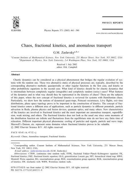
Physics Reports 371 (2002) 461–580www.elsevier.com/locate/physrepChaos, fractional kinetics, and anomalous transportG.M. Zaslavsky a;b;∗a Courant Institute of Mathematical Sciences, New York University, 251 Mercer Street, New York, NY 10012, USAb Department of Physics, New York University, 2-4 Washington Place, New York, NY 10003, USAReceived 1 July 2002editor: D.K. CampbellAbstractChaotic dynamics can be considered as a physical phenomenon that bridges the regular evolution of systemswith the random one. These two alternative states of physical processes are, typically, described by thecorresponding alternative methods: quasiperiodic or other regular functions in the rst case, and kinetic orother probabilistic equations in the second case. What kind of kinetics should be for chaotic dynamics thatis intermediate between completely regular (integrable) and completely random (noisy) cases? What featuresof the dynamics and in what way should they be represented in the kinetics of chaos? These are the subjectsof this paper, where the new concept of fractional kinetics is reviewed for systems with Hamiltonian chaos.Particularly, we show how the notions of dynamical quasi-traps, Poincare recurrences, Levy ights, exit timedistributions, phase space topology prove to be important in the construction of kinetics. The concept of fractionalkinetics enters a dierent area of applications, such as particle dynamics in dierent potentials, particleadvection in uids, plasma physics and fusion devices, quantum optics, and many others. New characteristicsof the kinetics are involved to fractional kinetics and the most important are anomalous transport, superdiusion,weak mixing, and others. The fractional kinetics does not look as the usual one since some moments ofthe distribution function are innite and uctuations from the equilibrium state do not have any nite time ofrelaxation. Dierent important physical phenomena: cooling of particles and signals, particle and wave traps,Maxwell’s Demon, etc. represent some domains where fractional kinetics proves to be valuable.c○ 2002 Elsevier Science B.V. All rights reserved.PACS: 05.45.+b; 47.52.+jKeywords: Chaos; Anomalous transport; Fractional kinetics∗ Corresponding author. Courant Institute of Mathematical Sciences, New York University, 251 Mercer Street,New York, NY 10012, USA.E-mail address: zaslav@cims.nyu.edu (G.M. Zaslavsky)Abbreviations: CTRW, continuous time random walk; FFPK, fractional Fokker–Planck–Kolmogorov equation; FK,fractional kinetics; FKE, fractional kinetic equation; GLG, generalization Lorentz gas; HIT, hierarchical island trap; MWE,Montroll–Weiss equation; RG, renormalization group; RGE, renormalization group equation; RGK, renormalization groupof kinetics; SW, stochastic web; WRW, Weirstrass random walk.0370-1573/02/$ - see front matter c○ 2002 Elsevier Science B.V. All rights reserved.PII: S0370-1573(02)00331-9

G.M. Zaslavsky / Physics Reports 371 (2002) 461–580 4639.2. Tangle islands ................................................................................. 5129.2.1. Accelerator mode island (standard map) .................................................... 5129.2.2. Accelerator mode island (web map) ........................................................ 5139.2.3. Ballistic mode island (separatrix map) ...................................................... 5149.3. Hierarchical islands trap (HIT) ................................................................... 5149.4. Stochastic net-trap .............................................................................. 5179.5. Stochastic layer trap ............................................................................ 51710. Dynamical traps and kinetics ......................................................................... 52010.1. General comments .............................................................................. 52010.2. Kinetics and transport exponents ................................................................. 52110.3. Estimates of the exponents ...................................................................... 52210.4. One-ight approximation ........................................................................ 52410.5. The 3/2 law of transport ........................................................................ 52610.6. Do the critical exponents exist? .................................................................. 52710.7. Straight denition of FKE exponents .............................................................. 52711. Dynamical traps and statistical laws ................................................................... 52811.1. Ergodicity and stickiness ........................................................................ 52811.2. Pseudoergodicity ............................................................................... 53011.3. Weak mixing .................................................................................. 53111.4. Maxwell’s Demon .............................................................................. 53211.5. Dynamical cooling (erasing of chaos) ............................................................. 53511.6. Fractal time and erratic time ..................................................................... 53711.7. Collection and interpretation of data .............................................................. 53811.7.1. Truncated distributions ................................................................... 53811.7.2. Flights and Levy Flights .................................................................. 53911.7.3. Elusive exponents ........................................................................ 53911.7.4. Monte Carlo simulation ................................................................... 53912. Fractional advection ................................................................................. 53912.1. Advection equations ............................................................................ 53912.2. Fractional transport by Rossby waves ............................................................. 54012.3. Hexagonal Beltrami ow ........................................................................ 54112.4. Three point vortices ow ........................................................................ 54312.5. Chaotic advection in many-vortices ow ........................................................... 54712.6. Finite-size Lyapunov exponents and stochastic jets .................................................. 55013. Fractional kinetics in plasmas ......................................................................... 55113.1. Fractional kinetics of charged particles in magnetic eld ............................................. 55113.2. Magnetic eldlines turbulence .................................................................... 55313.3. Test particles in self-consistent turbulent plasma .................................................... 55314. Fractional kinetics in potentials with symmetry .......................................................... 55414.1. Potentials with symmetry ........................................................................ 55414.2. Egg-crate potential .............................................................................. 55514.3. Fractional kinetics in other potentials ............................................................. 55614.4. Anomalous transport in a round-o model ......................................................... 55815. Fractional kinetics and pseudochaos ................................................................... 56115.1. Pseudochaos ................................................................................... 56115.2. Fractional kinetics and continued fractions in billiards ............................................... 56315.3. Maps with discontinuities ........................................................................ 56516. Other applications of fractional kinetics ................................................................ 56616.1. Fractional path integral .......................................................................... 56616.2. Quantum Levy ights ........................................................................... 56817. Conclusion ......................................................................................... 569

464 G.M. Zaslavsky / Physics Reports 371 (2002) 461–580Acknowledgements ..................................................................................... 569Appendix A. Fractional integro-dierentiation .............................................................. 569Appendix B. Useful formulas of fractional calculus ......................................................... 571Appendix C. Solutions to FKE........................................................................... 572References ............................................................................................ 5731. IntroductionBoltzmann was the rst who applied dynamical methods for a kinetic description of physicalobjects, beginning with his “Kinetic Theory of Gases” in 1895. The main feature of Boltzmann’smethod is the application of a probabilistic manner of description of particles simultaneously withthe original dynamical equations. This type of approach has become a standard one for large systemevolution and it is a crucial attribute to any kind of kinetic theory. Despite the fact that the Boltzmannequation was non-linear with respect to the distribution function, later linear types of kinetic equationswere derived, known now as balance or master equations. The main idea of the derivation ofa kinetic equation is to reduce the number of variables of complex systems by applying someassumption of the statistical or probabilistic type. Diusional equations can be considered as a simpleexample of kinetic equations, and their appearance is linked to the names of M. Smoluchowski, A.Einstein, M. Planck, and A. Kolmogorov. The presence of a probabilistic element in the derivation ofkinetic equations results in a possibility of another way of getting kinetics by a rigorous introductionof some stochastic process relevant to the described phenomena. As an elementary example, onemay consider the Gaussian process for a particle, wandering in a random media, with a beliefthat this is the adequate construction of particle motion. As a result, the diusion equation for aparticle’s distribution appears in a natural way as a consequence of the corresponding stochasticprocess.We use this trivial example to comment that the kinetic equation for real dynamical systemsappears as a compromise between two alternative types of descriptions: dynamical and statistical.Kinetic equations do not describe full dynamics, and some features of the dynamics can neverbe obtained from the kinetics. At the same time, kinetics always consists of constraints that cancontradict the dynamics and can exclude applicability of the corresponding stochastic process forsome domains of variables and parameters. We will provide many such examples in the correspondingsections.Dynamical chaos brings a new and immense area of research to the arena of the kinetic descriptionof physical objects. Applying a notion of “randomness” to the trajectories of chaoticdynamical systems, we have to admit that a kinetic description of “typical” chaos is at the beginningof its development. Chaotic dynamics possesses a number of peculiar features that requirea new approach in kinetics, in addition to the known tools, adjusted to complicated fractaland multi-fractal structures of phase space. Fractional kinetics (FK) (and, as a result, anomaloustransport) for Hamiltonian systems with dynamical chaos is the subject of this review. Althoughsome kind of fractional kinetics can be associated with the Levy process, the real kinetics for evenfairly simple models of chaos can be too far from the Levy process, preserving only some of itsfeatures.

G.M. Zaslavsky / Physics Reports 371 (2002) 461–580 465Considering trajectories of dynamical systems in phase space, we encounter very complicated andnot completely known topology even for the simplest cases with 1 1/2 or 2 degrees of freedom. Thephase space is non-uniform and consists of domains of chaotic dynamics (stochastic sea, stochasticwebs, etc.) and islands of regular quasi-periodic dynamics. Other topological objects such as cantoriand stable/unstable manifolds are also important to the study of kinetics. Trajectories, being consideredas a kind of stochastic process, do not behave like well known Gaussian, Poissonian, Wiener,or other processes. The dynamics is strongly intermittent and a topological zoo imposes a type ofkinetics with a wide spectrum of possibilities. Their classication has been started only recently, andmany specic and ne properties of the dynamics should be understood in the way of constructionof an adequate kinetics of chaos (for the earlier and some recent related reviews see, for example:Montroll and Shlesinger, 1984; Shlesinger, 1988; Bouchaud and Georges, 1990; Isichenko, 1992;Meiss, 1992; Wiggins, 1992; Shlesinger et al., 1993; Majda and Kramer, 1999; Bohr et al., 1998).The goal of this review is to present existing models of fractional kinetics and their connectionto dynamical models, phase space topology, and other characteristics of chaos. Section 2 consistsof preliminaries of the dynamics of chaotic motion. It describes some typical structures of phasespace and introduces important characteristics of chaotic dynamics: distribution of Poincare recurrencesand sticky domains. Section 3 consists of preliminaries for kinetics and basic constraints forthe FPK equation, that we call Kolmogorov condition. Section 4 describes the important Levy-typerandom process, its fundamental properties and generalizations. In Sections 5–8 we consider dierentaspects of FKE starting from its derivation, conditions of applicability, generalizations, probabilisticanalogs, and concluding by the renormalization group of kinetics. Sections 9 and 10 are related tospecic dynamical properties, dynamical traps, that inuence the transport and make it anomalousand imposes the fractional type of kinetics. All other Sections 11–16 are dierent applications of FK:Statistical laws in the cases of the presence of dynamical traps (Section 11); advection describedby FK (Section 12) and related issues in plasma physics (Section 13); particle dynamics in potentialswith dierent symmetry (Section 14). Special application of FK is in Section 15 where wediscuss systems with zero Lyapunov exponent but, nevertheless, with a kind of randomness calledpseudochaos. Particularly, such a situation occurs in dierent polygonal billiards, Lorentz gas, andthe vector eld lines behavior. Section 16 can be considered as an introduction to FK propertiesof quantum systems. The appendices have useful formulas of fractional calculus for the reader’sconvenience. There is no necessity to be familiar with fractional calculus for reading the review.2. Preliminaries: dynamics2.1. General commentsIn this section we consider some features of the chaotic dynamics which are relevant to the kineticdescription of a system. Equations of the Hamiltonian dynamics areṗ = −9H=9q; ˙q = 9H=9p ; (1)with generalized momentum p =(p 1 ;:::;p N ), coordinate q =(q 1 ;:::;q N ), and Hamiltonian H =H(p; q;t) which may depend on time t. The phase space of the system (p; q) has 2N dimensions,but even for N = 1 and time-dependent Hamiltonian, the systems of a general type have

466 G.M. Zaslavsky / Physics Reports 371 (2002) 461–580very complicated structure of phase space, where the domains of regular (non-chaotic) dynamicsalternate with the domains of erratic (chaotic) motion. It may not be so unexpected that kineticsin the domains of chaotic motion is not independent on what is happening near the chaos-orderborders.The task of describing the dynamics that, in some sense, has a seed of randomness, is not simpleand is not clear in many aspects. For example, all topological elements of phase space and theirproperties are not known and there is no complete scheme of the classication of the trajectories.We know about the existence of invariant curves (tori), stable/unstable manifolds, singular points orsurfaces, and cantori, but even a zero measure set of points of phase space can drastically changethe kinetics and transport properties of a particle. The concept of the neglecting of zero measure setsis typical for the ergodic theory of dynamical systems. The importance of some zero measure setsfor the kinetics goes far beyond the so-called “random phase” hypothesis widely used to describethe transition from dynamics to kinetics. It also means a necessity of the search for new classesof universality of kinetics, depending on the type of chaotic dynamics and phase space topology,and a necessity of the careful selection of a specic type of random process to describe the chaoticdynamics. We will demonstrate for such popular examples as the standard map or Sinai billiard howsome zero measure sets and ne features of the phase space topology come into account for thekinetic equations.2.2. Mapping the dynamicsDespite the fact that trajectories can be arbitrarily smooth, they can also display dierent fractalfeatures “extracted” after applying to the trajectories a specic algorithm. A trajectory can beconsidered not as a solution of the original Hamiltonian equations but, instead, as a solution of amap which is a set of discrete equations. This map should represent the trajectories, but part of theinformation about dynamics is hidden in the structure of the map. Maps are convenient for dierentsimplications of the dynamical equations. Below we show few examples of mapping the dynamics.2.2.1. Poincare mapThe Poincare map is a set of points in phase space (p; q) obtained from the intersection ofdirected trajectories with a hypersurface. The intersection points dene a set of time instants {t j } ofintersection. The map can be presented in the form(p n+1 ; q n+1 )= ˆT n (p n ; q n ); t n+1 = ˆf(t n ) (2)with an appropriate time-shift operator ˆT n and function ˆf. For 1 1/2 or 2 degrees of freedom andnite motion, the closure of the set (p i ; q i ) is an invariant curve or invariant torus if the dynamics isquasi-periodic, and it has randomly distributed points (stochastic sea) if the dynamics is chaotic. For ageneric situation, the Poincare map forms a stochastic sea with innite numbers of implanted islands.The dynamics in the islands is isolated from the dynamics in the stochastic sea and vice versa. Thedynamics inside the islands corresponds to the quasi-periodic trajectories as well as to the isolatednarrow stochastic layers with stochastic trajectories inside the layers. This intricate, sandwich-typestructure of phase space is at the heart of fractional dynamics. More about the Poincare map is inArnold (1978), and Lichtenberg and Lieberman (1983).

G.M. Zaslavsky / Physics Reports 371 (2002) 461–580 467Fig. 1. Poincare recurrences to the domain A.The Poincare map is the most eective for 1 1/2 or 2 degrees of freedom. The second equationin (2) for the mapping time is a source of serious complications unlesst n = t n+1 − t n = const: (3)for all n, or is approximately constant. The Poincare map will be considered in more detail later.2.2.2. Poincare recurrencesPoincare recurrences, or simply recurrences, is one of the most important notions for the kinetics.For a long time since the famous discussion between Boltzmann and Zermelo, the Poincarerecurrences did not play a serious constructive role in kinetics, although many derivations of thetransport equations involve the properties of periodic orbits and their distributions (see for example inBowen, 1972; Ott, 1993; Dorfman, 1999). Consider a domain A in phase space and a typical setof points {p; q ∈ A}. The Poincare theorem of recurrences states that for any initial condition of thetypical set, trajectories will repeatedly return to A if the dynamics is area preserving and conned.Let {t − j } be a set of time instants when a trajectory leaves A, and let {t+ j } be the set of time instantswhen a trajectory enters A (Fig. 1). The set{ (rec)j } A = {t − j − t − j−1 } A (4)is the set of recurrences. We call { (rec)j } the recurrence time at j-step, or the jth cycle. There aresome other characteristics related to the recurrences.Exit (escape) times can be introduced as a time interval between the adjacent entrances to A andexits from A:{ (esc)j } A = {t − j − t j + } A : (5)Similarly, one can introduce time intervals { (ext)j } that a trajectory spends outside of A duringone cycle:{ (ext)j } A = {t + j − t − j−1 } A : (6)

468 G.M. Zaslavsky / Physics Reports 371 (2002) 461–580There is an evident connection: (rec)j= (esc)j+ (ext)j : (7)The set of recurrence times { (rec)j } forms a specic mapping of trajectories. The sequence { (rec)j }can have fractal or multifractal features (Zaslavsky, 1995; Afraimovich, 1997; Afraimovich andZaslavsky, 1997, 1998). It also can be characterized by the probability distribution function P rec (; A).These properties of recurrences will be considered in Section 2.3. Similarly, one can consider themapping for { (esc)j } and { (ext)j }.2.2.3. Standard mapThe standard map is also known as the Chirikov–Taylor map (Chirikov, 1979). It is written formomentum p and coordinate x asp n+1 = p n + K sin x n ; x n+1 = x n + p n+1 ; (8)where K is a parameter that characterizes the force amplitude, and (p; x) are dened either on atorus (−¡p¡; −¡x¡), or on a cylinder (−∞ ¡p¡∞; −¡x¡), or in innitespace (−∞ ¡p¡∞; −∞ ¡x¡∞). The standard map has numerous applications in acceleratorphysics, plasma physics, condensed matter, etc. (see for example Chirikov, 1979; Lichtenberg andLieberman, 1983; Sagdeev et al., 1988). The map describes a periodically kicked rotor as well asmany other systems that can be reduced to the similar equation. Eqs. (8) are of the dierence type,while the original dierential equations are generated by the Hamiltonian:∞∑H = p 2 =2 − K cos x (t − m) : (9)m=−∞Map (8) has chaotic trajectories for any K. Domains of chaotic trajectories are bounded in thep-direction for K¡K c , forming a set of stochastic layers, and are unbounded in the p-directionfor K ¿ K c forming the so-called stochastic sea. The value of K c is known: K c =0:9716 ::: (seeGreene, 1979; Greene et al., 1981; Kadano, 1981; MacKay, 1983). Fig. 2 shows how complex isthe phase space structure of a “typical” dynamical system.2.2.4. Web mapThe web map appearing in Zaslavsky et al. (1986) for the study of charged particle dynamics ina constant magnetic eld and perpendicular electric wave packet. The Hamiltonian corresponds to aperiodically kicked linear oscillator:H = 1 2 (ẋ2 + ! 2 x 2 ) − K 0 cos x ∑(t − mT) : (10)m=−∞For the resonant condition !T =2=q and integer q, system (10) generates the so-called stochasticweb map of the q-fold symmetry in phase space (see more in Zaslavsky et al., 1991). For q =4,the corresponding map isu n+1 = v n ; v n+1 = −u n − K sin v n ; (11)

G.M. Zaslavsky / Physics Reports 371 (2002) 461–580 469Fig. 2. Phase portrait of the standard map (K =1:0).where we put ! 0 =1, K =2K 0 =, u =ẋ, v = −x. Again, as for the standard map, the region ofconsideration can be: a torus (u; v) ∈ (−; ); a cylinder u ∈ (−∞; ∞), v ∈ (−; ) oru ∈ (−; ),v ∈ (−∞; ∞); or innite (cover) space (u; v) ∈ (−∞; ∞). The stochastic web tiles innite space witha corresponding type of symmetry for any value of K (see Fig. 3). The channels of the web areexponentially narrow for K1 and narrow for K ∼ 1 (Fig. 3, part (a)). For K1, the stochasticsea covers full phase space leaving holes for islands that are lled by the nested invariant curvesand isolated stochastic layers (Fig. 3, part (b)).The main property of the web map (11) is that its phase space topology includes an unboundeddomain of chaotic dynamics for arbitrary value of the control parameter K, contrary to the standardmap. This makes the web map important to study of the unbounded transport of particles and thetransport dependence on the phase space topology.

470 G.M. Zaslavsky / Physics Reports 371 (2002) 461–580Fig. 3. Web map (K =1:5): (a) phase portrait; (b) formation of the web with 4-fold symmetry in the cover space(periodically continued in the both directions).2.2.5. Zeno mapThe Greek philosopher Zeno of Elea (circa 450 B.C.), is credited with creating several famousparadoxes, one of which, the “Achilles paradox”, was described by Aristotle in the treatisePhysics. The paradox concerns a race between the eet-footed Achilles (the Greek hero of Homer’sThe Illiad), and a slow-moving tortoise. The Achilles paradox postulates that as both start movingat the same moment, Achilles can never catch the tortoise, if the tortoise is given a head start. TheZeno map conveys this idea that Achilles can never catch the tortoise. It is a set of positions {x j },with Achilles initially at point x 0 , and the tortoise at point x 1 . When Achilles arrives at x 1 , the tortoiseachieves x 2 and evidently x 2 −x 1 x 1 −x 0 . When Achilles arrives at x 2 , the tortoise is at x 3 andx 3 −x 2 x 2 −x 1 , and so on. There is always a nite distance between Achilles and the tortoise whichis supposed to move with constant velocities. A solution for this paradox is in a special selection ofthe set of time instants t j that generate the map {x 0 ;x 1 ;:::}. This solution shows that not any mapof form (2) can represent dynamics which will adequately correspond to real trajectories or, simply,will adequately present the trajectories in phase space. This solution cautions us in the choice of amap that should replace real trajectories.2.2.6. Perturbed pendulumIt seems that the perturbed pendulum problem rst appeared in Landau and Lifshits (1976) in fewmodications:x + ! 0 2 sin x = j! 0 2 sin(x − t) (12)andx + ! 0[1 2 + j cos t] sin x = 0 (13)

G.M. Zaslavsky / Physics Reports 371 (2002) 461–580 471Fig. 4. Poincare map for the perturbed pendulum: (a) example of a stochastic layer with a sticky trajectory(j =7:86055; =8:57); (b) another example of the stochastic layer with dierent topology and almost invisibleislands.depending on the dynamics of the suspension point of the pendulum. The problem became a paradigmdue to its numerous applications (see a review in Zaslavsky et al., 1991). The Poincare map appearsas a set of points taken with time interval 2=, i.e. at t j =0, 1· 2=, 2· 2=;::: :In both Eqs. (12) and (13) there are two dimensionless parameters that control the phase spacetopology: j and =! 0 . Two examples in Fig. 4 show very dierent structures of the so-called stochasticlayers, elongated along x zones of chaotic dynamics. Transport of particles along x is dierentand depends on the topology, i.e. the transport is sensitive to the parameters j and =! 0 . Particularly,some dark regions indicate zones where a trajectory can spend a longer time than in other zones.This phenomenon is known as stickiness and it will be discussed later.2.3. Distribution of recurrencesBoltzmann was the rst who estimated the mean recurrence time for a gas model of particlesand showed that it is super-astronomically large. Boltzmann is also credited with the importantcomment that the Poincare theorem of recurrences does not involve anything related to the timeduration of the cycles. The important result on this issue was obtained by Kac (1958). Let P(; A)be the probability density to return to A at time ∈ (; +d). For small (A), P(; A) should beproportional to (A) if the system dynamics is area-preserving and bounded. More accurately, onecan introduce a probability densityP rec () =1lim P(; A) (14)(A)→0 (A)

472 G.M. Zaslavsky / Physics Reports 371 (2002) 461–580which exists and is normalized∫ ∞0P rec ()d =1 : (15)The mean recurrence time is rec = 〈〉 =∫ ∞0P rec ()d: (16)Due to the Kac lemma rec ¡ ∞ (17)for area-preserving and bounded dynamics (see also in Meiss, 1997; Cornfeld et al., 1982).Kac’s works on recurrences were the only ones with a new signicant result since a very long timeafter Poincare, Zermelo, and Boltzmann. The lack of interest in this subject could be explained bythe huge value of rec for the considered statistical models, so that there was no realistic possibilityto measure either rec or any eect related to the niteness of rec . The situation has been changedafter the discovery of chaos and its practical implementations.Chaos occurs in systems with a few degrees of freedom, starting from 1 1/2 degrees, and thetime of Poincare cycles becomes comparable to a characteristic time of the system. It was shownby Margulis (1969, 1970) that for systems with a uniform mixing property (Anosov-type systems):P()= 1 (exp − )(18) rec recwith rec =1=h ; (19)where h is Kolmogorov–Sinai entropy, or a characteristic rate of the divergence of close trajectory:r(t)=r(0) exp(ht) (20)with r(0) → 0 as an initial distance between any two trajectories, and r(t) as their distance attime t (see also in Zaslavsky, 1985).The exponential distribution of recurrences (18) is not the only possible one, and some simulationsshowed the possibility of an algebraic asymptotic distribution (Chirikov and Shepelyansky, 1984;Karney, 1983):P rec () ∼ 1= ( →∞) : (21)We call the recurrence exponent. It follows from the Kac lemma (17) that¿2 (22)(see also in Meiss, 1997; Zaslavsky and Tippett, 1991).Algebraic decay of P rec () is a result of a non-uniformity of phase space, and can be conjectured asa universal phenomenon for typical Hamiltonian systems with a stochastic sea and islands (Zaslavskyet al., 1997; Zaslavsky, 1999, 2002). A more accurate statement of this conjecture is that there existsat least a dense set of values of K for which1= 2 ¡P rec () ¡ 1= 1 ( →∞) (23)

with nite 1 ; 2 , and a non-uniform dependence ofG.M. Zaslavsky / Physics Reports 371 (2002) 461–580 473 1;2 = 1;2 (K) ; (24)where K is any control parameter of the system. This property will be discussed more in thecorresponding section and, particularly, it will be shown how the algebraic behavior of P rec () isrelated to fractal and multifractal properties of dynamics.2.4. Singular zonesThe studies of the chaotic dynamics by mathematicians and physicists was dierent from the verybeginning. While mathematicians were attracted by problems that permit a rigorous consideration(Anosov systems, Smale horseshoe Sinai billiard), physicists considered mainly the problems of animportant physical meaning such as the stability of particles in accelerators or the destruction ofmagnetic surfaces in toroidal plasma connement. We comment on this in order to continue thetreatment of some physically based conjectures which are directly related and important for physicalproblems but still do not have a rigorous foundation. As a part of this discussion is the origin offractional kinetics which prove to appear due to the non-uniformity of phase space.There are dierent reasons for the phase space non-uniformity. The main reason can be relatedto the existence of islands in any kind of domain of chaotic dynamics with a smooth Hamiltonian.The islands can be of dierent origin (resonances, bifurcations, etc.), and the phase space propertiesnear the islands’ boundaries are not well known (Meiss, 1986, 1992; Meiss and Ott, 1985, 1986;Rom-Kedar, 1994; Melnikov, 1996; Zaslavsky et al., 1997; Rom-Kedar and Zaslavsky, 1999). Inaddition to the islands, let us mention the so-called cantori-zero-dimension periodic sets that surroundislands, having an innite number of the cantor-set type holes and creating penetrable barriers fortransport (Percival, 1980; Meiss et al., 1983; Hanson et al., 1985).Here we would like to present only two examples. Both are related to the standard map (8), butcorrespond to dierent values of K. Fig. 5 shows a “griddle”-type vicinity of an island. The islandappears (and can disappear) as a result of a bifurcation from a parabolic point (Newhouse, 1977;Melnikov, 1996; Karney, 1983). The darkness of some domains in Fig. 5 indicates a long-term stayof the trajectory in the domain. Such phenomenon is called stickiness (Karney, 1983; Meiss and Ott,1985; Hanson et al., 1985). Another pattern of the stickiness is shown in Fig. 6 where a hierarchyof islands appears for a special value of K (Zaslavsky et al., 1997).A general feature of Hamiltonian systems is that their phase space is full of sticky domains whichwe call singular zones. They can be small and invisible in the Poincare maps, they depend on thecontrol parameters, and they can be modied in many ways, but their consideration is unavoidable fora general theory and they inuence kinetics and transport. For some earlier works on non-Hamiltoniansystems see Geisel (1984) and Geisel and Nierwetberg (1984).2.5. Sticky domains and escapesThe kind of stickiness imposes the type of anomalous transport. It can be that the sticky domaindoes not move with time or it does move in phase space. A trajectory that enters the sticky areaescapes from it after a very long time and this part of the trajectory represents a “ballistic” one thatcan be characterized by an almost regular dynamics with almost constant acceleration (stickiness to

474 G.M. Zaslavsky / Physics Reports 371 (2002) 461–580Fig. 5. A “net trap” example of a singular zone for the standard map with K =6:9009 after 10 9 iterations: (a) an islandthat is close to the bifurcation value of K; (b) magnication of the vicinity of the island.the accelerator mode island), or almost constant velocity (stickiness to the ballistic type island; seeSection 9). These are also sticky domains of other than accelerator or ballistic type (see Section 9).The origin of the stickiness does not have a universal scenario. A passage through the cantori wasdescribed in Meiss et al. (1983), Hanson et al. (1985), and Meiss and Ott (1985). Almost isolatedstochastic layers were considered in Petrovichev et al. (1990), Rakhlin (2000), and Zaslavsky (2002);islands-around-islands scenarios were considered in Meiss (1986, 1992), Zaslavsky et al. (1997), andRom-Kedar and Zaslavsky (1999); even one single marginal xed point can generate a stickiness andanomalous transport (Artuso and Prampolini, 1998). One can introduce a probabilistic description ofthe stickiness using escape rate probability P esc (t)dt that shows probability for a particle to escapea domain within the interval (t; t +dt), normalized as∫ ∞0dtP esc (t)=1 : (25)If asymptoticallyP esc (t) ∼ const:=t esc (t →∞) (26)and there is the only sticky domain with the escape exponent esc , then one may expect the followingrelation: = esc ; (27)where = rec (see (21)) is the exponent of distribution of recurrences, and consequentlyP rec (t) ∼ P esc (t) (t →∞) : (28)If there is more than one singular zone with dierent values of esc , then instead of (27), we have rec = min esc (t →∞) (29)

G.M. Zaslavsky / Physics Reports 371 (2002) 461–580 475Fig. 6. Hierarchy of islands 2–3–8–8–8–::: for the standard map for K =6:908745 (Zaslavsky et al., 1997).since the minimum value of esc denes the largest time asymptotics. A numerical example for thestandard map of the equivalence of two asymptotics (28), Fig. 7. After averaging over the numberof trajectories, the dierence between P rec for the probability density to return to the square A, andP targ of the probability density to leave A and reach rst time B, is indistinguishable. Both domainsA and B are in the stochastic sea and the majority of trajectories arrives rst time to B or returnsrst time to A after a fairly short time corresponding to law (18). After t rec there is a fairlysmall number of such trajectories. This group consists of trajectories that are visiting a singular zone

476 G.M. Zaslavsky / Physics Reports 371 (2002) 461–580Fig. 7. Targeting for the standard map: (a) location of the starting domain A st and the targeting domain A tg (both as blacksquares); (b) distribution of the P rec(t). Slope 1 is −2:19, slope 2 is −4:09. Distribution P targ(t) is almost indistinguishablefrom P rec(t). The data obtained after averaging over 3:22 × 10 9 initial conditions (Zaslavsky and Edelman, 2000).(see Fig. 8) on their way back to A (or to the target B). Just these delayed trajectories are responsiblefor the asymptotic behavior of P rec (t) and P esc (t).This simple comment implies a connection between singular zones and transport, that will bediscussed in dierent following sections.3. Preliminaries: kinetics3.1. General commentsA splitting of the dynamics into two dierent time-scales: short t and long col , is in the heartof the kinetic description of systems. Short time-scale is typically associated with the duration ofa “collision”, and long time-scale col corresponds to the interval between adjacent collisions. The“collision” should be considered in a broad sense: it may be a kind of essential change of energyor momentum due to an interaction with the external eld, or a change of variables due to the realcollision, or a strong change of the adiabatic invariants. Another important feature of the derivation ofthe kinetic equations is a reduction of the number of variables by an averaging over fast variable(s):P(p; t) ≡ TP(p; q; t)U ; (30)

G.M. Zaslavsky / Physics Reports 371 (2002) 461–580 477Fig. 8. Targeting without (top) and with (bottom) a singular zone Z. A trajectory escapes from the domain A and arrivesrst time to the domain B.where P is probability density, (p; q) are generalized momentum and coordinate correspondently, qis considered as the fast variable and double angular brackets denote averaging over q (see morefor the Hamiltonian chaotic dynamics in Zaslavsky, 1985). A typical time-scale connection reads:t col t : (31)Although conditions (31) are the most typical ones to obtain the kinetic equation for P(p; t), theexistence of singular zones and sticky domains imposes a number of deviations from the usualscheme. In this section will derive a regular diusion equation and compare the conditions of itsvalidity to the conditions of the derivation of the so-called fractional kinetic equation (FKE). We willalso make a comparison between the kinetics derived from the dynamics with the kinetics obtainedin the probabilistic way, the so-called Continuous Time Random Walk (CTRW) (see Montroll andWeiss, 1965; Montroll and Shlesinger, 1984; Shlesinger et al., 1987; Weiss, 1994). We will alsoindicate the conditions when the CTRW fails due to physical reasons.3.2. Fokker–Planck–Kolmogorov equation (FPK)The FPK equation was rst obtained by Fokker (1914) and Planck (1917). Kolmogorov (1938)derived a kinetic equation using a special scheme and conditions that are important for understandingsome basic principles of kinetics. Let W (x; t; x ′ ;t ′ ) be a probability density of having a particle atthe position x at time t if the particle was at the position x ′ at time t ′ 6 t. A chain equation of theMarkov-type process can be written for W (x; t; x ′ ;t ′ ):∫W (x 3 ;t 3 ; x 1 ;t 1 )= dx 2 W (x 3 ;t 3 ; x 2 ;t 2 )W (x 2 ;t 2 ; x 1 ;t 1 ) : (32)

478 G.M. Zaslavsky / Physics Reports 371 (2002) 461–580A typical assumption for W is its time uniformity, i.e.:W (x; t; x ′ ;t ′ )=W (x; x ′ ; t − t ′ ) : (33)Consider the evolution of W (x; x ′ ; t −t ′ ) during an innitesimal time t =t ′ −t and use the expansionW (x; x 0 ; t +t)=W (x; x 0 ; t)+ 9W (x; x 0; t)t + ··· : (34)9tEq. (34) is valid providing the limit:limt→01t {W (x; x 0; t +t) − W (x; x 0 ; t)} = 9W (x; x 0; t)9thas a sense. The existence of limit (35) for t → 0 imposes specic physical constraints that willbe discussed in this section later.Let us now introduce a new notation:P(x; t) ≡ W (x; x 0 ; t) ; (36)where the initial coordinate x 0 is omitted. With the help of Eqs. (32)–(34), we can transformEq. (35) into{ ∫}9P(x; t) 1= lim dyW(x; y;t)P(y; t) − P(x; t)9t t→0 t: (37)The rst important feature in the derivation of the kinetic equation is the introduction of two distributionfunctions P(x; t) and W (x; y;t) instead of the one W (x; p; x ′ ;p ′ ). The function P(x; t) willbe used for t →∞or, more accurately, for t which satises (31), where col is not dened yet. Inthis situation W (x; x 0 ; t) does not depend on the initial condition x 0 and this explains notation (36).Contrary to P(x; t), W (x; y;t) denes the transition during very short time t → 0: For t =0 itshould be no transition at all if the velocity is nite, i.e.:lim W (x; y;t)=(x − y) : (38)t→0Following this restriction we can use the expansion over the -function and its derivatives (Zaslavsky,1994a, b), i.e.:W (x; y;t)=(x − y)+A(y;t) ′ (x − y)+ 1 2 B(y;t)′′ (x − y) ; (39)where A(y;t) and B(y;t) are some functions. The prime denotes the derivative with respect tothe argument, and we consider the expansion up to the second order only.Distribution W (x; y;t) is called transfer probability and it satises two normalization conditions:∫W (x; y;t)dx = 1 (40)(35)and∫W (x; y;t)dy =1 : (41)

G.M. Zaslavsky / Physics Reports 371 (2002) 461–580 479The coecients A(x;t) and B(x;t) have a fairly simple meaning. They can be expressed asmoments of W (x; y;t):∫A(y; t)= dx(y − x)W (x; y;t) ≡ TyU ;∫B(y; t)=dx(y − x) 2 W (x; y;t) ≡ T(y) 2 U : (42)In a similar way, coecients for the higher orders of the expansion of W (x; y;t) can be expressedthrough the higher moments of W .Integration of (39) over x does not provide any additional information due to (40), but integratingover y and using (41) giveA(y;t)= 1 9B(y;t)(43)2 9yor applying notations (42)TyU = 1 92 9y T(y)2 U : (44)Expressions (43) and (44) were rst obtained in Landau (1937) as a result of the microscopicreversibility, or detailed balance principle. In Landau (1937), dynamical Hamiltonian equations wereused for (44), while here we use expansion (39) and “reversible” normalization (41). The nal stepis an assumption that we call Kolmogorov conditions: there exist limits:limt→0limt→01TxU ≡ A(x) ;t1t T(x)2 U ≡ B(x) ;1limt→0 t T(x)m U =0 (m¿2) : (45)It is due to the Kolmogorov conditions that irreversibility appears at the nal equation. Now it isjust formal steps. Substituting (39), (42), and (44) into (37) gives9P(x; t)9t= − 9 9x (AP(x; t)) + 1 29 2(BP(x; t)) (46)9x2 which is the equation derived by Kolmogorov and which is called the Fokker–Planck–Kolmogorov(FPK) equation. It is a diusion-type equation and it is irreversible. After using relations (43) and(44) we get the diusion equation (46) in the nal form:9P(x; t)9t9 9P(x; t)D9x 9x= 1 2with a diusion coecientT(x) 2 UD = B = limt→0 t(47): (48)

480 G.M. Zaslavsky / Physics Reports 371 (2002) 461–580Eq. (47) has a divergent form 1 that corresponds to the conservation law of the number of particles:9P9t = 9J(49)9xwith the particle uxJ = 1 2 D 9P9x : (50)In the following section we will see how a similar scheme can be applied to derive the fractionalkinetic equation.An additional condition follows from (44) and notations (45) and (48):A(x)= 1 29B(x)9x= 1 29D9xwhich explains a physical meaning of A(x) as a convective part of the particle ux. This part ofthe ux and A(x) are zero if D = const:3.3. Solutions and normal transportThere are numerous sources related to the solutions of FPK equation (47) for dierent initial andboundary conditions (see for example Weiss, 1994; Risken, 1989). Our goal here is just to mentiona few simple, important for the future, properties of the FPK equation.Let us simplify the case considering D = const:, x ∈ (−∞; ∞), and the initial condition for aparticle to be at x = 0. Then)P(x; t)=(2Dt) −1=2 exp(− x2; (52)2Dtknown as Gaussian distribution. Its odd moments are zero, second moment is〈x 2 〉 = Dt (53)and higher moments are〈x 2m 〉 = D m t m (m =1; 2;:::) (54)with D m=1 = D and D m¿1 can be easily expressed through D but they do not depend on t. Thereare two properties that we will refer to in the following section all moments of P(x; t) are nite, asa result of the exponential decay of P for x →∞, and the distribution P(x; t) is invariant under therenormalizationˆR(): x ′ = x; t ′ = 2 t (55)with arbitrary , i.e. the renormalization group ˆR() is continuous. Evolution of moments 〈x m 〉 withtime will be called transport. Dependence (53) and (54) will be called normal transport.(51)1 The way to derive Eq. (47) is slightly dierent from what has been used in the original works of Kolmogorov andLandau, due to the use of expansion (39) over the -function and its derivatives.

G.M. Zaslavsky / Physics Reports 371 (2002) 461–580 481Another type of the distribution function is the so-called moving Gaussian packet]P(x; t)=(2Dt) −1=2 (x − ct)2exp[− (56)2Dtwith a velocity c. Distribution (56) satises the equation9P9t + c 9P9x = 1 2 D 92 P(57)9x 2for which condition (43) or(51) fails. They can be restored if we consider the moments 〈(x −ct) m 〉.It follows from (56) thatand〈x〉 = ct (58)〈(x −〈x〉) 2 〉 = Dt (59)similarly to (53).3.4. Kolmogorov conditions and conict with dynamicsA perfect mathematical scheme often has constraints which limit its application to real phenomena.Constraints related to the Kolmogorov conditions (45) are very important for all problems relatedto the anomalous transport that will be discussed in the following part of this review. Consider thelimit t → 0 and an innitesimal displacement x along a particle trajectory that corresponds to thislimit. Then x=t → v where v is the particle velocity, and conditions (45) with notation (48) gives(x) 2 =t = v 2 t = D = const: (60)This means that v should be innite in the limit t → 0, which makes no physical sense.Another manifestation of the conict can be obtained directly from solution (52) to the FPKequation. This solution satises the initial conditionP(x; 0) = (x) (61)i.e. a particle is at the origin at t = 0. For any nite time t solution (52) or(56) has non-zeroprobability of the particle to be at any arbitrary distant point x, which means the same: the existenceof innite velocities to propagate from x =0 to x →∞during an arbitrary small time interval t.A formal acceptance of this result appeals to the exponentially small input from the propagationwith innite velocities. A physical approach to the obstacle in using the FPK equation is to abandonthe limit t → 0in(45), to introduce min t, and to consider a limitt=min t →∞: (62)A more serious question is how to use (62) and how the FPK equation can be applied to realdynamics. Let us demonstrate the answer using the standard map (8) as an example.As it was mentioned in Section 2.2.3, map (8) corresponds to a periodically kicked particledynamics, i.e. min t = 1 as it follows from (9). It is known from Chirikov (1979) that for K1

482 G.M. Zaslavsky / Physics Reports 371 (2002) 461–580one can consider variable x to be random with almost uniform distribution in the interval (0; 2). 2ThenTsin xU =0; Tsin 2 xU = 1 2 ;p n ≡ p n+1 − p n ; Tp n U =0; T(p n ) 2 〉〉 = K 2 =2 ; (63)where double brackets T :::U means averaging over x, and one can write the corresponding FPKequationwith9P(p; t)9t= 1 2 D(K)92 P(p; t)9p 2 (64)D(K)=K 2 =2 : (65)Eq. (64) provides the normal transport. Particularly〈p 2 〉 = 1 2 K 2 t: (66)More sophisticated analysis gives for D(K) an oscillating behavior( ) 1D(K)=K 2 2 − J 2(K)(67)with J 2 (K) as the Bessel function (see Rechester and White, 1980; Rechester et al., 1981), butkeeps the same diusional equation (64). More serious changes to the diusional equation will bediscussed in Section 10. Our main goal here is to show how the described conict can be eliminatedusing truncated distributions.3.5. Truncated distributionsA general scheme to perform a simulation of the problem of diusion and transport for givendynamical equations is to select a set of initial points in phase space {x 0 ;p 0 ;t =0} and let themmove until a large time t. Then for dierent time instants t 1 ;t 2 ;:::;t one can collect points intoboxes located in phase space and create a distribution function P(x; p; t j ) or its projections P(x; t j ),P(p; t j ). All these distributions are always truncated by some values x max , and p max because velocitiesof trajectories for all initial conditions are bounded during the nite time interval (0;t). For a fairlylarge t we can split, for example, P(p; t) into two parts:P(p; t)=P core (p; t)+P tail (p; t) (68)and calculate the corresponding moments〈p m 〉 = 〈p m 〉 core + 〈p m 〉 tail : (69)Let us estimate the second term in (69).2 Deviations from this approximation will be considered in detail later.

G.M. Zaslavsky / Physics Reports 371 (2002) 461–580 483Assume that p ∗ is the point of splitting of P(p; t) into the core and tail parts. Then∫ pmax〈p m 〉 tail = dpp m P(p; t) ¡ (p ∗ ) m P(p ∗ ;t)(p max − p ∗ ) : (70)p ∗For the Gaussian distribution P(p ∗ ;t) is exponentially small and we can neglect 〈p m 〉 tail independentlyon m. The situation is dierent if for large values of p the distribution function behavesalgebraically, i.e.P(p; t) ∼ c(t)=p p (p →∞) : (71)All moments 〈p m 〉 diverge for m ¿ p − 1 and estimate (70) should be replaced by〈p m c(t)〉 tail =m − p +1 pm−p+1 max →∞ (p max →∞) : (72)Expression (72) shows that for the truncated distribution with an algebraic asymptotics, the timeevolution of fairly large moments is dened through the largest value of momentum that a particlecan obtain during its dynamics. The result imposes some constraints on how large can m be for thegiven model with its p and for selected observation time t. Opposite to the Gaussian case, we canneglect 〈p m 〉 core in (69).A similar statement exists for another distribution function P(x; t) if its behavior is algebraic forlarge x¿0, i.e.P(x; t) ∼ c(t)=x x x →∞: (73)This consideration will be important when we consider anomalous transport in Section 10.The distribution dened as{P (tr) (p; t); 0 ¡p6 p max ;P(p; t)=(74)0; p¿ p maxwill be called truncated distribution, and the corresponding moments will be called truncatedmoments. Any kind of simulations of the direct dynamics deals only with the truncated distributionsand moments.Finally, we arrive at the following important constraints which are necessary for a realistic analysisof the dynamics:t ¿ t min (x; p) 6 (x max ;p max ) (75)which means the innitesimal time is bounded from below and the phase space variables are boundedfrom above. Other consequences of the truncation can be found in Ivanov et al. (2001).4. Levy ights and Levy processes4.1. General commentsGaussian distribution (52) links to the large numbers law: the sum of independent random variablesis distributed in the same way as any one of them. The uniqueness of the Gaussian distribution withsuch a property was reconsidered by Levy (1937) who had formulated a new approach valid for

484 G.M. Zaslavsky / Physics Reports 371 (2002) 461–580distributions with an innite second moment. There is a nice description of the history of Levy’sdiscovery, as well as its relation to other probabilistic theories and to the St. Petersburg paradox ofDaniel Bernoulli in Montroll and Shlesinger (1984). It happened that the Levy distribution and Levyprocesses had a strong impact on dierent areas of scientic analysis including not only probabilitytheory, but also physics, economics, nancial mathematics, geophysics, dynamical systems, etc. InFeller (1949), important theorems were formulated for the limit distributions (see Section 4.3).Mandelbrot (1982) has indicated numerous applications of the Levy distributions and coined a notionLevy ights. The more contemporary applications were analyzed in Montroll and Shlesinger (1984);Bouchaud and Georges (1990); Geisel (1995), and in a collection of articles by Shlesinger et al.(1995a, b). It became clear that the ideas related to the Levy processes can be important in theanalysis of chaotic dynamics after some modication will be applied (Zaslavsky, 1992, 1994a, b).In this section a very brief information about the Levy processes will be introduced with a stresson what are the features of the process that can be or cannot be used for the dynamically chaotictrajectories.4.2. Levy distributionLet P(x) be a normalized distribution of a random variable x, i.e.∫ ∞−∞P(x)dx =1 (76)with a characteristic functionP(q)=∫ ∞−∞dx e iqx P(x) : (77)Consider two dierent random variables x 1 and x 2 and their linear combinationcx 3 = c 1 x 1 + c 2 x 2 : (78)The law is called stable if all x 1 ;x 2 ;x 3 are distributed due to the same function P(x j ). Gaussiandistribution)P G (x)=(2 d ) −1=2 exp(− x2(79)2 dis an example of the stable distribution with a nite second moment d = 〈x 2 〉 (80)(compare to (52)). Another class of solutions was found by Levy (1937).Let us write the equation(P(x 3 )dx 3 = P(x 1 )P(x 2 ) x 3 − c 1c x 1 − c )2c x 2 dx 1 dx 2 ; (81)where condition (78) has been used. Following denition (77), one can write the equation forcharacteristic functionP(cq)=P(c 1 q)P(c 2 q) (82)

G.M. Zaslavsky / Physics Reports 371 (2002) 461–580 485orln P(cq)=lnP(c 1 q)+lnP(c 2 q) : (83)Eqs. (82) and (83) are functional ones with an evident solutionln P (cq)=(cq) = ce −i sign q |q| (84)and condition(c 1 =c) +(c 2 =c) = 1 (85)which consists of an arbitrary parameter .The distribution P (x) with the characteristic functionP (q) = exp(−c|q| ) (86)is known as Levy distribution with the Levy index . For =2 we arrive at the Gaussian distributionP G (x). An important condition introduced by Levy is0 ¡6 2 (87)which guarantee positiveness of∫P (x)= dq e iqx P (q) : (88)This condition will be discussed later in Section 5.The case = 1 is known as Cauchy distributionP 1 (x)= c 1 x 2 + c : (89)2An important case is the asymptotics of large |x|P (x) ∼ 1 1c () sin (90) 2 |x| +1(see Levy, 1937; Feller, 1949, 1957; Uchaikin and Zolotarev, 1999).4.3. Levy processThere are many dierent ways to introduce the Levy process, i.e. a time-dependent process thatat an innitesimal time has the Levy distribution of the process variable (Levy, 1937; Gnedenkoand Kolmogorov, 1954; Feller, 1957; Uchaikin and Zolotarev, 1999; Montroll and Shlesinger, 1984).Here we use a simplied version for the innitely divisible processes.Consider the transition probability density P(x 0 ;t 0 ; x N ;t N ) that satises the chain equation∫P(x 0 ;t 0 ; x N ;t N )= dx 1 :::dx N−1 P(x 0 ;t 0 ; x 1 ;t 1 ) · P(x 1 ;t 1 ; x 2 ;t 2 ) :::P(x N−1 ;t N−1 ; x N ;t N ) (91)and putt j+1 − t j =t; (∀j); t N − t 0 = N t : (92)

486 G.M. Zaslavsky / Physics Reports 371 (2002) 461–580Assume that the process is uniform in time and space, i.e.P(x j ;t j ; x j+1 ;t j+1 )=P(x j+1 − x j ; t j+1 − t j )=P(x j+1 − x j ;t) : (93)Then (91) transforms into∫P(x N − x 0 ; N t)= dy 1 ::: dy N P(y 1 ; t) :::P(y N ;t) ; (94)where y j = x j − x j−1 ; j ¿ 1.By introduction the characteristic functions∫P(q)= dy j e iqyj P(y j ;t) (j ≠ N ) ;∫P (N ) (q)=we obtain from (94)dy (N) e iqy(N ) P N (y (N) ; N t); y (N) =N∑y j (95)P N (q)=[P(q)] N : (96)Following the concept of stable distributions and using expression (82), let us consider P(q) asafunction of two parameters and c that will be dened later. Namely, change the notationP(q) → P (q;c); P N (q) → P (q; c N ) ; (97)where c or c N should replace c in (86). These equations are consistent ifc N = Nc = N t · c ≡ cN t (98)tand Eq. (96) takes the formP (q; ct) = exp(−cN t|q| ) (99)with t = Nt and t 0 = 0. In the limit t → 0, N →∞, N t = t, and c =c=t we arrive to thecharacteristic function of the Levy process:P (q; t) = exp(−ct|q| ) : (100)The original Levy process can be written as the inverse Fourier transform of (100)∫P (x; t)= dq e iqx−ct|q| (101)with the asymptotics for |x| →∞similar to (90)P (x; t) ∼ 1 c () sin 2 · t: (102)|x|+1From (102) we have for the moment of order m (not necessarily integer)〈|x| m 〉 = ∞; m¿ : (103)The second moment (m=2) is innite since ¡2 (see more about similar derivations in Zaslavsky,1999; Yanovsky et al., 2000).1

G.M. Zaslavsky / Physics Reports 371 (2002) 461–580 4874.4. GeneralizationsThere are dierent generalizations of Levy distributions and Levy processes that can be useful inapplications. Mainly they are related to anisotropy of the distributions. For examplewithP (q; ; c) = exp{−c|q| [1+i sign q · tan(=2)]}; ≠1; 0¡¡2 (104) = c+ − c −c + + c − ; c= a (c + + c − ) ; (105)where a is dened by the normalization condition and for = 1 tan(=2) should be replaced by(=2) ln |k| (see in Cizeau and Bouchaud, 1994; Yanovsky et al., 2000; Uchaikin, 2000). Distribution(104) provides asymptoticsP (x; ; c) ∼ c ± =|x| +1 : (106)Streaming distributionP (x; t) ∼ const:=|x − vt| +1 (107)was considered in Montroll and Shlesinger (1984). Another important generalization, the so-calledLevy walks (Shlesinger et al., 1987) will be considered in Section 6.4.5. Poincare recurrences and Feller’s theoremsIn this section we describe a few results formulated in Feller (1949). They show a connectionbetween the Levy processes and Poincare recurrences. Although these results are not related directlyto dynamical systems, the Poincare recurrences distribution plays an important role in kinetics as wewill see it in Sections 9–12. From that point, Feller’s theorems are a “half-way” to the dynamics.Consider a small domain A (see Fig. 1) and recurrences to A. The recurrence time is the timeinterval between two subsequent crossings of the boundary of A by a trajectory of the particle onits way out of A. In the bounded Hamiltonian dynamics the sequence of recurrence times {t j }≡t 1 ;t 2 ;:::;t n ;::: is innite. It is assumed that t j are mutually independent and they belong to the sameclass of events with all identical probability distribution functionP rec () = Prob{t k = } (∀k) (108)i.e. independent on k. The integrated probability of recurrences isP intrec(t)=∫ t0dP rec () (109)and∫ ∞F(t)=1− Prec(t)=int dP rec () (110)thas a meaning of a probability that the recurrence time is ¿ t.

488 G.M. Zaslavsky / Physics Reports 371 (2002) 461–580Feller (1949) introduced two additional characteristics of the recurrences chain: sum of n recurrencetimesS n = t 1 + ···+ t n (111)and number of the recurrences N t during time interval (0;t). An evident connection between themisProb{N t ¿ n} = Prob{S n 6 t} : (112)Due to the Kac lemma (17) the mean recurrence time rec is nite. Then under the conditions ofindependence of t j and niteness of rec , two following theorems are valid (Feller, 1949):1. If 2 ¡ ∞ then for every xed ∫ Prob{S n − n rec 6 n 1=2 } →()=(2) −1=2 dy exp(−y 2 =2)−∞{}1=2 Prob N t ¿ t= rec − t → () ; (113)rec3=2where 2 = 〈(t k −〈t k 〉) 2 〉 = 〈(t k − rec ) 2 〉 (114)and the connection from (112) has been usedn rec + n 1=2 = t: (115)A simple meaning of this theorem is that uctuations of the recurrence time from its mean value rec are distributed due to the Gaussian law.2. Let F(t) in(110) has the asymptoticsF(t)= 1 h(t); 0 ¡¡2 (116)t withlim h(cx)=h(x)=1 :x→∞Then for 1 ¡¡2{Prob N t ¿ t= rec −b }t → P rec(1+)= () ; (117)i.e. to the Levy distribution with P () from (90) and b t to be obtained from the equationF(b t ) ∼ 1=t 1= :Distribution (117) isthe only possible non-normal distribution for N t and 1 ¡¡2.The last statement of the Feller’s theorem does not leave us any possibility to escape the Levydistribution for physical problems since the condition of the theorem are fairly broad. We do notput the case 0 ¡¡1 since it is forbidden due to the Kac lemma. Indeed, comparing (21), (110)and (116) we obtain = − 1 and condition (22) means ¿1.The presented theorems extend our information about a universality of distribution of the recurrencetimes uctuations as random variables: for a nite dispersion 2 they are distributed due to the

G.M. Zaslavsky / Physics Reports 371 (2002) 461–580 489Gaussian law, and for an innite dispersion due to the Levy law. Nevertheless, analysis of thechaotic dynamical systems does not show this, although the Gaussian or Levy distributions cansometimes be a good approximation.4.6. Conict with dynamicsThere are dierent observations that the recurrences distribution can be of the algebraic type (21)with ¿ 3or ¿ 2 if we apply the notations of the Feller’s theorems with a corresponding Levyindex. These observations were obtained by simulation (see, for example, in Zaslavsky and Niyazov,1997; Zaslavsky et al., 1997; Rakhlin, 2000; Leoncini and Zaslavsky, 2002). Another example, Sinaibilliard (Sinai, 1963) with innite horizon, seems to have = 3 and ¿2 up to a logarithmic factorwhat follows from a qualitative analysis and simulations (Bunimovich and Sinai, 1973; Geisel etal., 1987b; Zacherl et al., 1986; Machta, 1983; Machta and Zwanzig, 1983; Zaslavsky and Edelman,1997). One can expect dierent deviations from (117) if we recall that the condition of independencyof the recurrence times {t j } in Section 4.5 is a kind of approximation in dynamical systems withchaos. Typically there are correlations between the neighboring steps of Poincare maps that areimportant for kinetics. Due to that there is a possibility of deviations from the Levy distributionand Levy process, and more general approach is necessary. In other words, the Levy’s idea ofdistributions with innite moments can be valid with some restrictions. This issue will be discussedin Section 10.5. Fractional kinetic equation (FKE)5.1. General commentsHaving in mind a description of chaotic trajectories, we can consider rst a situation when thecomplexity (Badii and Politi, 1997) of the trajectories have a hierarchical structure. For example, atrajectory can be presented with dierent levels of accuracy, or dierent levels of coarse-graining Sin phase space and t in time. The more complicated the details, the higher the level of complexity.While trajectories can be arbitrary smooth, their approximation can be a singular one and may requirecorrectly dened conditions of the applicability. The hierarchical sequence of curves can be continuedup to some level n after which the property of occurrence of more and more smaller details stopsdue to physical reasons. Nevertheless we can consider a formal limit n →∞of the hierarchicalcomplexity, and arrive in that way to a singular fractal representation of the trajectories which will bevalid up to the sizes ‘¡‘ 0 . The gain of considering singular trajectories instead of the smoothones is in a simplication of the theory by introducing some invariant features of dynamics, namelyrenormalization group approach. This section consists of such a type of approach to the kineticsof chaotic dynamics, based on the results of Zaslavsky (1992, 1994a, b). The derived equation iscalled Fractional Fokker–Planck–Kolmogorov Equation (FFPK) or simply fractional kinetic equation(FKE). We also will use the notion of fractional kinetics (FK).The idea of exploiting fractional calculus and presenting kinetics in a form of an equation with fractionalintegro-dierentiation is not new. For example some variants of FK were used in Mandelbrotand Van Ness (1968) for signals; Young et al. (1989) for kinetics of advected particles; Isichenko

490 G.M. Zaslavsky / Physics Reports 371 (2002) 461–580(1992) and Milovanov (2001) for the problem of percolation; Hanson et al. (1985) for kineticsthrough cantori for the standard map; Nigmatullin (1986) for the porous media; Douglas et al.(1986, 1987) in macromolecules (see also a review paper by Douglas, 2000); Hilfer (1993, 1995a, b)for evolution and thermodynamics; West and Grigolini (2000) for time series. We will also presenthere some ideas for the solution of FKE based on Saichev and Zaslavsky (1997) as more motivatedfor the dynamical systems analysis. Additional material can be found in Hilber (2000) and in Metzlerand Klafter (2000). The necessary material on fractional calculus is in the appendices.5.2. Derivation of FKEFollowing Zaslavsky (1992, 1994a, b), we provide in this section a simplied version of the FKE.Let us assume that the transition probability W (x; x 0 ; t +t) with an innitesimal t has a newexpansion, instead of (34) and (35):limt→01|t| {W (x; x 0; t +t) − W (x; x 0 ;t)}= 9 W (x; x 0 ; t)9t = 9 P(x; t)9t (0 ¡6 1; t¿ 0) ; (118)where we use notation (36) and properties of fractional derivatives (see Appendix A). We alsointroduce the expansion for W (x; y;t) instead of (39):W (x; y;t)=(x − y)+A(y;t) () (x − y)+B(y;t) (1) (x − y) (0¡¡ 1 6 2)(119)with appropriate fractal dimension characteristics and 1 . It is still possible to write for the coef-cient B(y;t) its denition through a moment of W :∫T|x| 1 U ≡ dx |x − y| 1 W (x; y;t)= (1 + 1 )B(y;t) (120)which is similar to (42) but the coecient A(y; t) does not have so simple interpretation for thegeneral case unless B =0.By integrating (119) over y we obtain a relation9 A(x)9(−x) + 91 B(x)=0 ; (121) 19(−x)whereA(x; t)A(x) = limt→0 (t) B(y;t)B(x) = lim =t→0 (t) 1(1 + 1 ) lim T|x| 1 U(122)t→0 (t) similar to (35). Eq. (121) is a generalization of (43) for the detailed balance principle. Existence oflimits (122) when t → 0 is instead of the Kolmogorov conditions (45). Fractional values of , 1and represents a new type of the fractal properties of the coarse-grained dynamics.

G.M. Zaslavsky / Physics Reports 371 (2002) 461–580 491A particular case is 1 = + 1, and (121) transforms into[9 A(x) − 9B(x) ]=0 (123)9(−x) 9xequivalent to (51) withB(x)=1(2 + ) lim T|x| +1 U;t→0 (t) 1A(x)=(1 + ) lim T|x| U(124)t→0 (t) and the generalization of the Landau formulas (43) and (44):t → 0: T|x| U(t) =(1 + )(2 + )9 T|x| +1 U: (125)9x (t) The existence of limits (124) can be considered as generalized Kolmogorov condition (compareto (45)).The FKE can be derived from (118) rewritten on the basis of (32):9 P(x; t)9t = limt→0{∫1(t) or using expansion (119) and denitions (122)}dy [W (x; y; t +t) − (x − y)]P(y; t)(126)9 P(x; t)= 9(A(x)P(x; y)) +91(B(x)P(x; y)) : (127)9t 9(−x) 19(−x)This equation can be simplied in the case 1 = +1(9 P9t = − 9B 9P )(128) 9(−x) 9xwhich transfers into regular diusion equation for = 1 and B = 1 2 D.Fractional derivatives are well dened in a specied direction (see Appendix A), and there is nosimple replacement x →−x or t →−t. That is why a more general operator should be considered,for example, instead of the derivative of order one can considerˆL x () = A + 9 =9x + A − 9 =9(−x) : (129)For a symmetric case one can use Riesz derivative[ ]9 9|x| = − 1 9 2 cos(=2) 9x +9( ≠1): (130) 9(−x) The corresponding FKE (127) takes the form (Saichev and Zaslavsky, 1997)9 P9t = 9 9|x| (AP)+91 9|x| (BP); 0 ¡¡ 1 1 6 2 : (131)

492 G.M. Zaslavsky / Physics Reports 371 (2002) 461–580In the case, when the term with B can be neglected, we have a simplied version of FKE9 P9t = 9(AP) : (132) 9|x|In the case =1, = 2 it is a normal diusion equation. For 0 ¡¡1, =29 P9t = 92(AP) (¡1) (133) 9x2 it is called the equation of fractional Brownian motion (Mandelbrot and Van Ness, 1968; Montrolland Shlesinger, 1984). For = 1 and 1 ¡¡2 the FKE corresponds to the Levy process (seeSection 4.3):9P9t =9(AP) (1¡¡2) : (134)9|x|There are other dierent forms for the FKE that generalize forms (131) and (134): anisotropicequations were considered in Yanovsky et al. (2000); Meerschaert et al. (2001); directioned equations(Weitzner and Zaslavsky, 2001; Meerschaert et al., 2001); non-linear fractional equations (Bileret al., 1998; Barkai, 2001; Schertzer et al., 2001). Some of these equations will be considered later.We should mention that the investigation of the type and properties of the FKE is at its beginningstage and a number of important questions are not answered yet. Some of these questions will bediscussed in the following sections.Parameters ; ; 1 will be called the critical exponents.5.3. Conditions for the solutions to FKEAny type of the FKE and its generalization can be considered as independent mathematical problems.If we want to stay closely to the specic applications of the FKE to dynamical systems,restrictions related to the physical nature and the origin of the FKE should be imposed. Before consideringsolutions to the FKE, let us make a few comments about some constraints. Other conditionswill be done later.(a) Interval condition. We should dene interval of consideration in space–time. Speaking aboutthe space, we have in mind phase space (coordinate–momentum) and the variable x can representany of them. The innite intervals assume a possibility to have innite moments of P(x; t) whilenite intervals (x min ;x max ), (t min ;t max ), that will be called space and time windows, lead to the allnite moments since P(x; t) is integrable.(b) Positiveness. Solution P(x; t) has the meaning of probability, and it should be positivelydened, i.e.P(x; t) ¿ 0 (135)in the domain of consideration. For the innite space–time domains condition (135) leads to restrictionson the possible values of critical exponents. Particularly we have the condition 0 ¡6 2 forthe Levy processes ( = 1) or the condition:0 ¡6 1; 0 ¡6 2 (136)

G.M. Zaslavsky / Physics Reports 371 (2002) 461–580 493(Saichev and Zaslavsky, 1997) for (132) with A = const: A rigorous consideration of the P(x; t)positiveness for both fractal values of (; ) does not exist yet. Examples of the violation of (136)will be shown later.(c) Intermediate asymptotics. It can be that dynamics imposes dierent asymptotics for dierentspace–time windows. An example of particles advection in convective ow can be found in Younget al. (1989). Other examples will be indicated later. For such cases should be dierent pairs ( j ; j )for dierent windows.(d) Evolution of moments. It is easy to obtain the time-dependence of some moments if A=const:in (132). Let us multiply the equation by |x| and integrate it over x. Then9 〈|x| 〉9t ∫= A∫= A 9P(x; t)dx |x|9|x| dxP(x; t) 99|x| |x| = A (1 + ) ; (137)where we introduce the moment of P(x; t)∫〈|x| 〉 = dx |x| P(x; t) (138)and use the formulas from Appendix A. After integrating (137) over t (or dierentiation withrespect to t − ) we obtain〈|x| (1 + )〉 = A(1 + ) t : (139)For the case of the self-similarity of the solution for FKE, which we will discuss more inSection 5.4, one may expect〈|x|〉 ∼ t = = t =2 ; (140)where we introduce the transport exponent ≡ 2= : (141)(e) Denition of fractional integro-dierentiation. This denition is not unique (Samko et al.,1987) and there is a discussion of using dierent denitions for space and time derivatives (Chukbar,1995). In fact, one can use any integral transform and a type of the chosen derivative will inuenceboundary-initial conditions and the way how the solution P(x; t) will be constructed by the inversetransform. More accurately, one can say that the distribution P(x; t) is dened not only by theboundary-initial conditions but also by the type of derivatives used in FKE. A similar situationexists with Fourier or Laplace transforms. Any of them can be used if we know how to select acontour of integration in the complex plane to satisfy the boundary-initial conditions.5.4. Solutions to FKE (series)In this section we consider FKE in the form9 P(x; t)=9P(x; t)+S(x; t) ; (142)9t 9|x|

494 G.M. Zaslavsky / Physics Reports 371 (2002) 461–580where S(x; t) is a source. For the source we use the standard formS(x; t)=(x)(t) (143)or a time distributed point sourceS(x; t)=S 0 (t)(x) ;S 0 (t)=t − = (1 − )= 99t ˆ1 → →1 (t) (144)which will be explained later and where{1; t¿0 ;ˆ1=0; t¡0 :There are two ways to proceed: using innite series (Saichev and Woyczynski, 1997; Saichev andZaslavsky, 1997; Zolotarev et al., 1999), or using Fourier–Laplace transform (Afanasiev et al., 1991;Fogedby, 1994; Compte, 1996; Meerschaert et al., 2001; Weitzner and Zaslavsky, 2001).Consider a Fourier transform with respect to xP(q; t)=∫ ∞−∞and similarly for source (144)S(q; t)=∫ ∞−∞dx e iqx P(x; t) (145)dx e iqx S(x; t)=S 0 (t) : (146)Eq. (142) transforms into9 9t P(q; t)+|q| P(q; t)=S 0 (t) (t¿0) : (147)For case (146) solution for (147) can be written in the form (Saichev and Zaslavsky, 1997)∞∑ (−1) mP(q; t)=(m +1) (|q| t ) mwhereE (z)=m=0= E (−|q| t ) (t¿0) ; (148)∞∑z m = (m + 1) (149)m=0is the Mittag–Leer function of order (see Appendix C).Using the inverse transformP(x; t)=∫ ∞−∞dq e −iqx P(q; t) (150)we can write the solution in the series formP(x; t)= 1|y|1t =2∞ ∑m=0(−1) m|y| m (m +1)(m +1) cos [ 2 (m +1) ]; (151)

whereG.M. Zaslavsky / Physics Reports 371 (2002) 461–580 495y = x=t =2 (152)and is the same as in (141). The asymptotics of (151) isP(x; t) ∼ 1 under conditiont (1 + ) sin|x| +1 (1 + ) 2(153)|x| 2 t : (154)Expression (153) coincides for = 1 with the Levy process distribution P (x; t) in(102). We canconclude from (153) that the moments〈|x| 〉 ¡ ∞ if 0 ¡¡6 2 : (155)Series (148) also shows that the solution can be considered in a self-similar formP(x; t)=t −=2 P (;) (|x|=t −=2 ) (156)which we will discuss later. For =2, 6 1 all moments 〈x m 〉 are nite.5.5. Solutions to FKE (separation of variables)This section having more technical details, provides an important physical interpretation of theFKE (Saichev and Zaslavsky, 1997).Consider Laplace in time and Fourier in space transforms of P(x; t):P(q; u)=∫ ∞0dt∫ ∞−∞dx e −ut+iqx P(x; t) (157)with the inverse formulaP(x; t)= 1 ∫ c+i∞∫ ∞du2i c−i∞ −∞dq e ut−iqx P(x; t) : (158)Application of (157) to the FKE (142) with source (143) givesP ; (q; u)=1=(u + |q| ) (159)(see Appendix B for integral transforms of fractional derivatives). This result can be rewritten inthe form∫ ∞∫ ∞P ; (q; u)= ds exp[ − s(u + |q| )] = dsQ (u; s)W (q; s) (160)00withQ (u; s)=e −su ; W (q; s)=e −s|q| : (161)Q (u; s) and W (q; s) can be interpreted as corresponding Levy-type characteristic functions with aparameter s, and (160) is separation of variables formulae for the characteristic function P ; (q; u)of the solution.

496 G.M. Zaslavsky / Physics Reports 371 (2002) 461–580withLet us apply now the inverse transform (158) and use presentation (160):P ; (x; t)=∫ ∞0dsQ (t; s)W (x; s) (162)∫ c+i∞∫ c+i∞Q (t; s)= 1 du e ut Q (u; s)= 1 du exp(ut − su ) ;2i c−i∞2i c−i∞∫ ∞∫ ∞W (x; s)= dq e −iqx W (q; s)= dq exp(−iqx − s|q| ) : (163)−∞−∞Result (162) completes the separation of variables and presents the solution through a superpositionof Levy processes along x and t. A similar presentation can be developed for the more complicatedsource (144) (see also Afanasiev et al., 1991; Fogedby, 1994; Compte, 1996).5.6. Conict with dynamicsThe limitations for application of the FKE to dynamical systems can be compared to the limitationsfor diusional process described in Section 4.6. Consider analogs (124) and (125) to the Kolmogorovcondition (45):(x) =(t) = v (t) − = A = const: (t → 0) : (164)At the same time, − = (1 − =)=(1 − =2) ¿ 0 (165)since ¡2. This means that in the limit t → 0 should be v →∞, and we arrive at the sameconict as in the normal diusion case. The resolution of this conict is similar to the case of normaldiusion: there exists t min such that for t ¡ t min the FKE cannot be applied.More serious constraints are imposed by the condition of positiveness of P ; (x; t), i.e. ¡1,0 ¡¡2. Some simulations show, as we will see later, the values ¿2. A theory of the FKE isnot developed yet for ¿1 and ¿2.We also need to consider truncated distribution function{P(tr);P ; (x; t)=(x; t); 0 ¡x6 x max ;(166)0; x¿ x max(compare to (3.5.7)) and truncated moments∫〈|x| m 〉 tr =dxP (tr);(x; t) ¡ ∞ (167)in order to avoid innite velocities in the solutions, forbidden by the dynamics. All these commentswill be necessary when real experimental or simulation data are compared to the theory. As it followsfrom (156)〈|x| m 〉 tr ∼ t m=2 (168)

G.M. Zaslavsky / Physics Reports 371 (2002) 461–580 497and all truncated moments are nite, although there is a restriction on the value of m which dependson t max (see the discussion in Section 3.5). Particularly〈|x| 2 〉 tr ∼ t (169)introducing the transport exponent .For = 1 we have the Levy process with =2= ¡ 2. This means that the permitted values of are1 ¡¡2 (170)and it is not clear from the dynamics why the values of 0 ¡¡1 are not achievable. For the interval(170) ¿1, i.e. the transport is superdiusive, and it is not clear from the dynamics if subdiusivetransport with ¡1 is forbidden or not, while the subdiusion was observed in Schwagerl and Krug(1991) and in Afanasiev et al. (1991). The value = 2 corresponds to the pure ballistic case. Thiswill be discussed more in Section 9.5.6. Probabilistic models of fractional kinetics6.1. General commentsWe use the notion “probabilistic models” to underline the fact that the main axiomatic approachto the nal kinetic equation is based on the construction of random wandering process rather thanon the construction of a model for dynamic trajectories. The most popular and widely used is theso-called Continuous Time Random Walk (CTRW) model introduced in Montroll and Weiss (1965)and developed in a number of succeeding publications (Weiss 1994; Montroll and Shlesinger, 1984;Shlesinger et al., 1987; Uchaikin, 2000; Metzler and Klafter, 2001). Some other models alsowill be considered in this section and their relations to each other will be discussed.6.2. Continuous time random walk (CTRW)CTRW theory operates with two kinds of probabilities related to the random walk of a particle:probability density to nd a particle at the position x after executing j steps P j (x), and probabilitydensity to nd a particle at x at time t; P(x; t). The corresponding random walk equations assumeindependence of changes at each step together with a uniformity of the probability distributions oftime and distance intervals between consequent steps. Under these conditions we have for P j (x)P j+1 (x)=∫ ∞−∞dx ′ W (x − x ′ )P j (x ′ ) (171)with W (x) as a transitional probability, andP(x; t)=∫ t0d(t − )Q(x; ) (172)with (t) as a probability density to stay in the achieved position x for a time t, and Q(x; t) asaprobability to nd a particle in x at t immediately after a step has been taken.

498 G.M. Zaslavsky / Physics Reports 371 (2002) 461–580The probability (t) can be expressed through the probability density (t) to have an interval tbetween two consequent steps:(t)=∫ ∞tdt ′ (t ′ ) : (173)Let j (t) be the probability density to make the jth step at a time instant t. Thenj+1(t)=∫ t0d (t − ) j (); 1 (t) ≡ (t) : (174)The following obvious equation:∞∑Q(x; t)= j(t)P j (x) (175)j=1establishes the connection between discrete steps random walk and continues waiting time at dierentsteps.It is convenient to use Fourier transforms of P j (x) and W (x):P j (q)= 1 ∫ ∞dx e iqx P j (x) ;(2)−∞∫ ∞W j (q)= 1 dx e iqx W (x) (176)(2) −∞which for simplicity are written in one-dimensional case. From (171) and (176) we obtainP j (q)=W (q)P j−1 (q)=[W (q)] j (177)with an initial condition P 0 (q) = 1, i.e. the particle is initially at the origin. Thus, from (177)P j (x)=∫ ∞−∞dx e −iqx [W (q)] j : (178)Consider Laplace transform of j (t); (t) and Q(x; t):j(u)=(u)=∫ ∞0∫ ∞0dt e −ut j(t) ;dt e −ut (t) ; (179)∫ ∞Q(x; u)= dt e −ut Q(x; t) :0Then it follows from (174) and (179)j(u)= (u) j−1 (u)=[ (u)] j : (180)

After combining (172), (179) with (175) we obtain∫ ∞G.M. Zaslavsky / Physics Reports 371 (2002) 461–580 499e −iqxQ(x; u)= dx−∞ 1 − W (q) (u) : (181)Finally, using connection (173) in the form(u)=[1− (u)]=u (182)and applying it and (181) to(172) we arrive at the solution:P(x; t)= 12i∫ c+∞−i∞du 1 u [1 − (u)]eut × 12∫ ∞−∞dqe −iqx1 − (u)W (q)(183)which the Montroll–Weiss equation (MWE). The nal result has been expressed through the twobasic probabilities: W (x) for the length of a step, and (t) for the time interval between the consequentsteps.There are numerous investigations of the MWE (Weiss, 1994; Montroll and Shlesinger, 1984;Metzler and Klafter, 2000), as well as its generalization (Shlesinger et al., 1987; Uchaikin, 2000).6.3. Asymptotics for CTRWThe main applications of the MWE are related to the limits t →∞; x →∞and correspondingapproximations with two transition probability functions (u) and W (q) which forms a considerablemodel of the random walk process. By choosing (u) and W (q) one can create a model thatpresumably should t the physical situation. Eq. (183) is just a formal presentation of the solutionsthat can be very dierent depending on the model functions W (q) and (u). Let us rewrite (183)in the form[1 − (u)W (q)]P(q; u)= 1 [1 − (u)] (184)uand consider some cases for (u) and W (q). For example we can assume that(u)=1+t 0 u; W (q)=1+x 0 q − 1 2 q2 (185)considering the limits u, q → 0 equivalent to the limits t →∞, x →∞, and introducing constantst 0 ;x 0 , and . Then, up to the higher orders terms, (184) becomes(t 0 u + x 0 q − 1 2 q2 )P(q; u)=t 0 (186)which is equivalent to the diusion equationt 09P(x; t)9t+ x 09P(x; t)9xIt is also assumed that t 0 , ≠0.Consider now the case= 1 2 92 P(x; t)9x 2 + t 0 (x)(t) : (187)W (q)=1−|q| ; (u)=1− u (u; q → 0) (188)

500 G.M. Zaslavsky / Physics Reports 371 (2002) 461–580(Afanasiev et al., 1991; Weiss, 1994; Uchaikin, 2000), where constants are included into the denitionof q and u. Substitution of (188) into (184) gives(u + |q| )P(q; u)=u −1 ; (189)where we neglect the product u |q| ,orandP(q; u)=P(x; t)= 12u−1u + |q| (190)12i∫ c+i∞c−i∞∫ ∞du−∞u−1dqu + |q| : (191)The last expression can be used to obtain the moments 〈|x| 〉. By replacing the variables we canobtain〈|x| 〉 = const: t = = const: · t =2 (192)(Afanasiev et al., 1991). This result coincides with (140) for the FKE. In fact, it is a consequenceof the Eq. (189) that coincides with (142) if the source will be taken in form (144). To prove this,let us use the formulas of the Laplace–Fourier transforms of the derivatives (see the Appendix B):d (F)g(x) →−|q| g(q) ;d|x|d (L)g(t) → u g(u) ; (193)dt d (L) ˆ1 → u −1 ;dt where (F) and (L) indicates Fourier and Laplace transforms. Applying (193) and (144) to Eq. (189),we arrive at9 P(x; t)9t = 9 P(x; t)9|x| +t (x) (194)(1 − )which coincides with the FKE (140) when the source is taken in the special form (144). This resultestablishes the connection between the FKE and CTRW as well as dierences since the equationsare obtained in dierent approximations and dierent initial assumptions. For example the MWEequation (184) or(183) is fairly general and does not use approximations q → 0, u → 0 while thetransition to FKE does. At the same time, in the limit q → 0, u → 0 MWE has a special type ofsource (144) while the FKE does not specify the source. In addition, the FKE in form (194) or(190) can be valid not only in the limit q → 0, u → 0 but for fairly small time–space scales as wewill see for dynamical systems.6.4. Generalizations of CTRWThere are few generalizations that enhance possible applications of the CTRW theory: they areLevy walk (Shlesinger et al., 1987), relativistic model of CTRW (Shlesinger et al., 1995a, b),

G.M. Zaslavsky / Physics Reports 371 (2002) 461–580 501multiplicative random walks (Shlesinger and Klafter, 1989), and others. Here we would like to stopbriey on the so-called Levy walk which was introduced in Shlesinger et al. (1987) in order toavoid innite moments of the displacement x. In the same scheme of derivation of the CTRW, leta probability density (x; t) to make a jump of the length x in a time t is(x; t)= (t|x)W (x) ; (195)where W (x) has the same meaning as in (171) and (x|t) is a conditional probability. It is alsopossible to write(x; t)=W (x|t) (t) (196)with (t) the same as in (173) and W (x|t) as a conditional probability.As a simple demonstration, consider an expression(t|x)=(t − x=V (x)) ; (197)where V (x) is a velocity as a function or the displacement. This form appeared in Shlesinger andKlafter (1989) to show that for the Kolmogorov scaling V (x) ∼ x 1=3 and W (x) ∼|x| 1+ one couldnd for the mean square displacement x(t):⎧t ⎪⎨3 ; 6 1=3 ;〈x(t) 2 〉 = t 2+(3=2)(1−) ; 1=3 6 6 1=2 ;(198)⎪⎩t; ¿ 1=2 :The idea of the Levy walk is to couple space-time memory by using expressions (195)–(197) andto obtain, in this way, the nite second moment of the displacement at time instant t while thedistribution of all possible displacements W (x) has innite second moment (see more discussions ofthat in Section 5.6).One additional type of generalization of the CTRW can be useful for applications. This is relatedto the so-called master equation. It was proposed in Montroll and Shlesinger (1984) to write themaster equation in the form9P(x; t)9t∫ {t∑= d(t − ) W (x − x ′ )P(x ′ ;t) − P(x; )0x ′}(199)with an appropriate transition probability W (x) and a delay probability function (t − ). Following(182) and (188), we can assume that (u) ∼ u or (t) ∼ 1=t 1+ .A generalized fractional Kolmogorov–Feller equation was proposed in Saichev and Zaslavsky(1997):9 P(x; t)9t =∫ ∞−∞which is similar to (199).dyW(t)[P(x − y; t) − P(x; t)] (200)

502 G.M. Zaslavsky / Physics Reports 371 (2002) 461–5806.5. Conict with dynamicsThe CTRW or MWE equation are governed by two arbitrary probabilistic functions W (x) and(t), and there are high resources for applications when these probabilities appear from knownprocesses. Chaotic dynamics, in its contemporary stage, does not provide information about W (x)and (t) except for maybe some special solutions. In lieu of this comment, one should be verycareful in applying the CTRW to experimental and simulation data. The best example is related tothe basic assumption for the derivation of the CTRW equation: independence of steps in the randomwalk (see Section 6.2), which denitely is not the case for the standard map, web map, and allother more complicated models of chaos. A similar comment can be made for the Levy walk. Thedynamic equations and, for example, the standard map do not impose the relation of (195)–(197)type and the observations of many other dynamical models show an absence of the strong couplingof (197) type (see for example in Kuznetsov and Zaslavsky, 2000).7. More fractional equationsLiterature related to the equations with fractional derivatives is fairly vast. Although it is not asubject of this review, we would like to mention some publications that can be important in thestudy of dynamics: general approach to the media with a fractal support, such as the porous media(Nigmatullin, 1986); fractional wave equation (Wyss, 1986; Schneider and Wyss, 1989; Mainardi,1996a, b); dierent equations including fractional dierences (Mainardi, 1997; Goreno et al., 1999);stable distributions and related equations (Uchaikin, 2000; Uchaikin and Zolotarev, 1999); asymmetricgeneralization of the FK (Yanovsky et al., 2000). In this section we will consider only a fewdierent cases that seems to be important for applications to the dynamics.7.1. Weierstrass random walk (WRW)The Weierstrass random walk (WRW) was coined in Hughes et al. (1981) (see also Montroll andShlesinger, 1984). Although the WRW is not as well known as CTRW and it is not as convenientfor an immediate implementation, it contains the most important feature of the FK in a very explicitform, namely self-similarity, scalings, and renormalization group equation.In the following we use the presentation from Montroll and Shlesinger (1984). Consider a randomwalk on a one-dimensional periodic “lattice” with a spacing one and a probability p j to make a stepof the length a j . Then probability density to make a step of the length ‘ isP(‘)= 1 2∞∑p j [(‘ − a j )+(‘ + a j )] (201)j=1if the random walk is symmetric, and∫ ∞−∞d‘P(‘)=1 : (202)

504 G.M. Zaslavsky / Physics Reports 371 (2002) 461–580with some exponent and non-singular function Q(k). That is enough to conclude that 0 ¡¡2since the regular part of (207) has only even powers of k, and that Q(k) should be periodic in ln kwith a period ln a that follows from (210). After substitution of (212) in(210) we also obtain = |ln p|=ln a: (213)A straightforward way is to apply the inverse Mellins transform to cos (a n k)in(207):P(k)= 1 − p ∞∑∫ c+i∞p j (s) cos(s=2)ds= 1 − p ∫ c+i∞(s)|k| −s cos(s=2)ds(214)2ia sj |k| s 2i1 − p=a sj=0c−i∞(see Hughes et al., 1981, 1982; Montroll and Shlesinger, 1984). The numerator has poles at s =0; −2;:::; and the denominator has poles ats j =lnp=ln a ± 2ij=ln a = − ± 2ij=ln a: (215)The nal result from (214) and (215) is obtained by application of the residues over all poles:∞∑P(k)=1+|k| (−1) n k 2nQ(k)+p(2n)!(1 − pa 2n ) ;Q(k)= pln a∞∑n=−∞n=1c−i∞(s n ) cos(s n =2) exp(−2in ln |k|=ln a) (216)in full correspondence with (201) and (213).We deliberately stop on the details of the WRW since it will be shown in the following sectionshow many similar features can be found in FK of systems with dynamical chaos. Particularly we haveto stress attention on the so-called log-periodicity of the singular part P s (k) through the function Q(k)with respect to the variable k which was well known in the RGT of phase transitions (Niemeijerand van Leeuwen, 1976) but did not play as essential role as it did in the dynamical systemstheory (Benkadda et al., 1999; Zaslavsky, 2000a). For other applications of the log-periodicity seeSornette (1998).7.2. Subdiusive equationsWhile the diusion equation has a xed form, the form of fractional kinetics is not prescribedand there exists a possibility of numerous fractional formats depending on physical situations. Forexample, numerous variants of kinetics can appear if we modify expansions (118) and (119) ormake special selections of the basic spectral functions (u);W(q) in(183) for the CTRW (Montrolland Shlesinger, 1984; Afanasiev et al., 1991; Chukbar, 1995; Compte, 1996; Saichev and Zaslavsky,1997; Uchaikin, 1999, 2000).As an example, instead of (185) consider1= (u)=1+u ; u → 0 (0¡6 1) ;W (q)=1+x 0 q − 1 2 q2 : (217)

G.M. Zaslavsky / Physics Reports 371 (2002) 461–580 505Then P(q; u) satises the equation(u + x 0 q + 1 2 q2 )P(q; u)=u (218)or in (x; t) variables9 P(x; t) 9P(x; t)+ x9t 0 = 1 9x 2 2 92 P(x; t)+9x 2t (x) (0¡6 1) : (219)(1 + )This equation, that corresponds to the fractal Brownian motion (Mandelbrot and Van Ness, 1968),can be generalized to the three-dimensional random walk:9 P(r;t)+ v ·∇P(r;t)=DP(r;t)+ t−(r) (0¡6 1) (220)9t (1 − )(Compte, 1996; Uchaikin, 2000; Weitzner and Zaslavsky, 2001).As it was mentioned in Section 5.4, for case (219) all moments 〈x m 〉 are nite. The function (u)in (217) is a characteristic of delays or traps with a probability density to stay time t before theescape(t) ∼ 1=t 1+ ; t →∞: (221)This probability has innite mean time of escapet esc ≡〈t〉 =∫ ∞0t (t)dt (222)for ¡1, imposing innite recurrence time. Such a situation should not appear in Hamiltoniandynamics. At the same time, Eq. (219) provides〈x 2 〉 =(1 + ) t (0 ¡6 1) (223)that corresponds to the subdiusion (Saichev and Zaslavsky, 1997). The Hamiltonian phase spaceis at least two-dimensional, and the subdiusion along one variable and superdiusion or diusionalong the other one are not forbidden. Just this case of subdiusion in Hamiltonian dynamics wasobserved in Afanasiev et al. (1991), Schwagerl and Krug (1991) and Benenti et al. (2001).7.3. SuperdiusionIn FK the second moments 〈 2 〉 of some physical variable can be innite as it is for the Levyprocesses. In a fairly general situation we can use expression (140)〈||〉 ∼ t = = t =2 ; (224)where we replace x by an abstract . The transport exponent (see (141)) is dened in a way asthe second moment is nite,〈 2 〉∼t : (225)The case with = 1 corresponds to the normal diusion, ¡1 is subdiusion, and ¿1 is superdiusion.All these denitions assume self-similarity if we use denition (224), and a possibility

506 G.M. Zaslavsky / Physics Reports 371 (2002) 461–580of using (225) at least for the truncated moments, i.e.〈 2 〉 tr ∼ t (226)(compare to (169)). Dynamical systems, even fairly simple at rst glance, display a rich set ofdierent possibilities: the value of can be very close to one, but the dynamics can be too far fromthe Gaussian process, self-similarity can be valid in some restrictive way and can be applied not forall moments, etc. We will meet these examples in the following sections.A simplied version of superdiusion can be introduced directly as (134) or(139)or9P(; t)9t= A 9 P(; t)9|| (227)〈|| 〉 = (1 + )At ; (228)where we put A = const:; = 1, and replace x by . Expression (228) implies in the case ofself-similarity =2= ¿ 1 (229)since ¡2. A similar result comes from (153) ifweput =1.All these situations were considered in numerous publications (Montroll and Shlesinger, 1984;Afanasiev et al., 1991; Fogedby, 1994; Chukbar, 1995; Compte, 1996; Saichev and Zaslavsky, 1997).We should comment that the superdiusion can also exist for ¡1. An interesting situation appearsin the case when there are few dierent directions of diusion. In Hamiltonian dynamics there areat least two directions: along the coordinate and along the momentum. In such a case〈| e (0)|〉 ∼ D e (0)t (e(0) )=2 ; (230)i.e. the transport exponent depends on the direction of transport, given by the unit vector e (0)(Chernikov et al., 1990; Petrovichev et al., 1990; Weitzner and Zaslavsky, 2001; Meerschaert andScheer, 2000; Uchaikin, 1998). In this way the FK imposes a new type of the anisotropy whichreveals not only in the diusion constant D e (0) but also in the transport exponent (e (0) ). It followsfrom the Kac lemma that at least in one direction should be the superdiusion (see also a commentat the end of the previous section.Generalization of the FK for the anisotropic case can be performed in dierent ways (Zolotarevet al., 1999; Weitzner and Zaslavsky, 2001).The simplest form (Compte, 1996; Yanovsky et al., 2000; Zolotarev et al., 1999) is to use theRiesz fractional derivative for the fractional Laplace operator(−) =2 F→|k|(231)dened through its Fourier transform. Explicit expression for the fractional Laplacian is more complicated(see the Appendix B). Using expression (231) one can write down the generalized FKE9 F(r;t)= D9t (−) =2 f(r;t) : (232)Dierent asymptotic solutions for (232) are given in Zolotarev et al. (1999) and Weitzner andZaslavsky (2001).

G.M. Zaslavsky / Physics Reports 371 (2002) 461–580 5078. Renormalization group of kinetics (GRK)Renormalization group (RG) is a powerful tool to study physical phenomena with scaling properties(see for example in Kadano, 1981, 1993, 2000; Greene et al., 1981; MacKay, 1983; Hentscheland Procaccia, 1983; Jensen et al., 1985). Initially, the methods of RG proved to be ecient in theeld theory and statistical physics and later they were applied to dynamics and chaos. The Gaussianprocess can be considered as a rst and trivial example of a possible application of RG theory inthe kinetics, and crucial achievements were obtained for the kinetics near a phase transition point(Wilson and Kogut, 1974; Hohenberg and Halperin, 1977). Chaotic dynamics near the so-calledcantori exhibits scaling properties and the corresponding kinetic equation was derived by Hanson etal. (1985) (see also MacKay et al., 1984). An important feature of RGK is the coupling of space–time scalings. This coupling has pure dynamical origin and it imposes a necessity to go deeply intounderstanding of the dynamical singularities (see Sections 2.4 and 2.5) in order to nd the linksbetween spatial and temporal behavior of trajectories. The material of this section follows Zaslavsky(1984a, b), Zaslavsky (2000a) and Benkadda et al. (1999).8.1. Space–time scalingsLet ‘ be a space variable and t be the time variable so that P(‘; t) is a density distribution alongthe dynamical trajectories. Consider an innitesimal change of P(‘; t) in time, i.e. t P(‘; t)=P(‘; t +t) − P(‘; t) (233)and the corresponding to t innitesimal change in space ‘ P(‘; t)= ∑ ‘[P(‘ +‘; t) − P(‘; t)] ; (234)where the sum is performed over all possible paths of the displacement ‘ during the same timeinterval t. Fractal properties of the chaotic trajectories can be applied directly to (233) and (234) t P =(t) 9 P9t ; ‘ P = ∑ ‘9 9‘ (|‘| A ′ P) ; (235)where ; are critical exponents that characterize the fractal structures of space–time, ‘ is assumedto be positive (length of a “ight”), and A ′ is a function of ‘ and other phase space variablesadditional to ‘.A typical kinetic equation appears as a balance equation t P = ‘ P; (236)where the bar means averaging over all possible paths and additional to ‘ variables. Using a notationA ≡ ∑ ‘|‘| (t) A′ (237)

508 G.M. Zaslavsky / Physics Reports 371 (2002) 461–580we arrive from (236) to9 P9t = 9(AP) (238)9‘i.e. to a simplied version of the FKE (134) with ‘ = |x|.The RGK can be introduced starting from the dynamics. Let the dynamics carry the rescalingpropertiesˆR K :‘ → ‘ ‘; t → T t; (239)which one may accept in a broad sense, i.e. the rescaling exists after some averaging, coarse-graining,in restricted time–space domains, etc. The basic feature of the RGK is that the balance equation(236) is invariant under the renormalization transform (239), i.e.ˆR K t P = ˆR K ‘ P (240)which means that9 P9t = ‘9 (AP) 9‘T(241)Starting from some minimal values t, ‘, one can apply ˆR K arbitrary number n times. Thistransforms (241) into( ) n9 P9t = ‘ 9 T(AP) : (242)9‘The kinetic equation (238) “survives” under action of ˆR K if the limit n →∞has a sense, i.e. ifthere exists a limitlim n→∞ ( ‘= T )n =1 (243)which leads to the xed point solution= =ln ‘ =ln T ≡ =2 : (244)Eq. (244) shows an important connection between the exponents (; ) and scaling constants ( ‘ ; T ).This result can be expanded to a more fundamental property if we consider the moment equationfor (238), i.e.〈‘ 〉 = D t (245)(compare to (139)) with(1 + )D =(1 + ) A : (246)Comparing (244) to(141) we obtain that is the transport exponent =2ln ‘ =ln T (247)which is now expressed through the scaling parameters ( ‘ ; T ).

G.M. Zaslavsky / Physics Reports 371 (2002) 461–580 5098.2. Log-periodicityThe existence of FKE is based on the formal existence of the limitlim A′ |‘| =(t) = const: (248)t→0which is equivalent to the Kolmogorov condition for the FPK equationlimt→0 (‘)2 =t = const: (249)The essential dierence, in addition to the dierence of the exponents, appears when we imposeinvariance of the FKE under the RG-transform ˆR K . Indeed, expression (249) is invariant under thetransformˆR G :‘ → 1=2 ‘; t → t (250)with arbitrary value of . That means that the Gaussian renormalization ˆR G is continuous, whilethe ˆR K is discrete with xed values of ‘ and T . As a result, a new property of the solution ofFKE occurs known as log-periodicity (see a review article on log-periodicity by Sornette (1998) andapplication to FKE in Benkadda et al. (1999) and Zaslavsky (2000a)).The FKE (238) is linear and a sum of its solutions is also a solution. Particularly, xed-pointequation (243) has innite number of solutions. For example, k = ln ‘ =ln T +2ik=ln T = 1 2 +2ik=ln T (k =0; ±1;:::) (251)satises (243) and expression (244) gives a particular solution only for k = 0. Using (251), we canrewrite the moment equation (245) in the form of the superposition∞∑∞∑( )〈‘ 〉 = D (k) t k= D (0){1+2} t (D (k)2k =D(0) ) · cos ln t ; (252)ln Tk=0k=1where new coecients D (k)(k¿0) are unknown and typically are small. The term in braces isperiodic with respect to ln t and the period isT log =ln T : (253)Fig. 9 provides an example of log-periodicity for the web map of the 4th order symmetry. Moreexamples appear in the forthcoming section.For the cases when the initial kinetic equation has a discrete renormalization invariance in anexplicit form the coecients D (k)can be explicitly calculated (Hanson et al., 1985; Montroll andShlesinger, 1984; see also Section 7.1 on WRW). Another comment is related to the limit t → 0in (248). When the RG is discrete, there are cut-o values of min ‘ ≡ ‘ 0 and min t ≡ t 0 , andall other permitted values of ‘; t are greater or much greater of ‘ 0 ; t 0 . A physical meaningof them will be given in Section 9. Some other application of the log-periodicity can be found inShlesinger and West (1991).

510 G.M. Zaslavsky / Physics Reports 371 (2002) 461–580Fig. 9. Log-log plots of the even moments M 2m = 〈R 2m 〉 of the trajectories displacement R vs. number of iterations (time)N for the web map with 4-fold symmetry and K =6:25, top, with normal diusion, and K =6:349972, bottom, withsuperdiusion (Zaslavsky and Niyazov, 1997).

G.M. Zaslavsky / Physics Reports 371 (2002) 461–580 5118.3. Multi-scalingFor a general dynamics of even low-dimensional systems, calculations with only two scalingexponents and is a fairly strong simplication. Multi-scaling dynamics is a more adequate formof dynamics, and the log-periodicity can be considered as an example of the reduced multi-fractality.Multi-scaling can occur either from a singular zone or from several singular zones. A general ideaof the multi-fractality was developed in Grassberger and Procaccia (1984), Parisi and Frisch (1985),Jensen et al. (1985), Halsey et al. (1986) and Paladin and Vulpiani (1987).It is assumed the existence of many dierent exponents, say dierent , with a distribution function(). We can use again the property of linearity of the FKE and consider its solution as P(‘; t; )and the normalization condition∫ ∞ ∫d()P(‘; t; )=1 : (254)‘ min =‘ 0d‘Expression (245) for the moments should be modied as∫ ∞ ∫〈‘ 〉 = d ()D t P(‘; t; ) : (255)‘ 0d‘All the following steps are fairly formal depending on the functions (), D (k), etc., and as in manytypical situations, properties of () permit to apply the steepest descent method to perform andintegration over . This procedure will select a special value (or a few of them) for which theunder-integral extremum appears (see for details in Zaslavsky, 2000b).9. Dynamical traps9.1. General comments and denitionsIn Sections 2.4 and 2.5 we have preliminary discussions of such properties of dynamics as singularzones and stickiness. This section considers these notions in more details using a more comprehensivephenomenology of dynamical traps. We pursue an idea that kinetics and transport of chaotic systems,in general, can be evaluated when the phase space topology is fairly well known. In other words,while a “microscopic” theory of kinetics in statistical physics is based on our knowledge aboutthe acting forces, in the kinetic theory of dynamical chaos, one should go further and deeper andunderstand the phase space topology that depends on the system’s parameters values and that canvary for the same type of the acting forces. Dynamical trap is, perhaps, the most important partof the topology-transport connection, that is a long standing problem of physics and mathematics(Hanson et al., 1985; Meiss and Ott, 1985; Meiss, 1992; Wiggins, 1992; Rom-Kedar et al., 1990;Haller, 2000, 2001a, b; Melnikov, 1996; Zaslavsky, 1984; Chernikov et al., 1990; Rom-Kedar andZaslavsky, 1999; Zaslavsky, 2002).The trap, in its absolute meaning, does not exist in Hamiltonian dynamics due to the Liouvilletheorem on the phase volume preservation. In Section 2.3 we have introduced the distribution functionP(A; t) of Poincare recurrences to a domain A. Dynamical trap of an order m 0 ¿ 1 is dened as

512 G.M. Zaslavsky / Physics Reports 371 (2002) 461–580a domain A m0 such that m (A m0 ) ≡〈t m 〉 = 1 ∫ ∞t m P(A m0 ;t)dt = ∞ (m ¿ m 0 ¿ 1) ; (256)(A m0 ) 0where the value m 0 may be a non-integer. The domain A m0 is a singular zone. A system may havemany singular zones and one can expect the asymptotics of the (21) typeP rec (A m0 ;t) ∼ 1 t (257)with = (A m0 ). For the normalized distribution of recurrences P rec (t) (see (14)), one can writeP rec (t) ∼ ∑ jc j =t (Aj) (258)indicating that dierent singular zones with their own recurrence exponents make input into the nalasymptotics. As t →∞, the lowest value of the recurrence exponent for P rec (t) survives whilefor dierent time intervals can be dierent intermediate asymptotics and dierent values of (seeSections 2.3 and 2.4). It can also be more complicated non-algebraic forms of P rec (t).There is no classication of singular zones or dynamical traps. A general comment is that anyboundaries or singular sets (singular points) can play such a role. In this section we provide aqualitative description of three types of possible traps (Zaslavsky, 2002) and estimate their relationto the kinetics and transport problems.9.2. Tangle islandsThe islands of the so-called accelerator mode and ballistic mode were called tangle islands inRom-Kedar and Zaslavsky (1999) to distinguish them from the resonance islands. Stickiness oftrajectories to the boundaries of tangle islands leads to the superdiusion (Zaslavsky and Niyazov,1997; Zaslavsky et al., 1997; Iomin et al., 1998). Here we provide a few examples of the tangledislands (see also Sections 2.4 and 2.5).9.2.1. Accelerator mode island (standard map)For the standard map (8) an accelerator mode island appears for K in the intervals2m 6 K 6 2m +K(m) ; (259)where m is an integer and K(m) is an interval of the existence of the corresponding island. Thereare other intervals of K where there are accelerator mode islands of higher orders (see more inLichtenberg and Lieberman, 1983). For the values of K in (259), starting from x 0 = =2;p 0 =0, aparticle moves with the linearly growing value of p n :p n =2m (260)that explains the name of the island. The island collapses atK =[4 2 +(2m) 2 ] 1=2 : (261)

G.M. Zaslavsky / Physics Reports 371 (2002) 461–580 513Fig. 10. Accelerator mode islands for the web map with K =6:28318531.An eective Hamiltonian of regular trajectories inside the island can be written as (Karney, 1983)H (a) = 1 2 (p)2 +(K − K c )x − 3 (x)3K c =2m; x = x − x (a) ; p = p − p (a) (262)and x (a) ;p (a) represents the trajectory with K = K c ;x 0 = =2;p 0 =0.9.2.2. Accelerator mode island (web map)It is a similar type of islands for map (11). An example of the value of K c isK c =2;u (a)0= =2; v (a)0=3=2 (263)which generates the trajectory (u n(a) ;v n (a) ). The eective Hamiltonian is (Zaslavsky and Niyazov, 1997)H (a) = 1 2 (K − K c)(v − u) − 6 [(v)3 − (u) 3 ] (264)(see Fig. 10). The islands appear for K¿K c and correspond to some degenerate case.

514 G.M. Zaslavsky / Physics Reports 371 (2002) 461–5809.2.3. Ballistic mode island (separatrix map)This example appears in Rom-Kedar and Zaslavsky (1999) for the separatrix map (Zaslavsky andFilonenko, 1968):h n+1 = h n + jK n sin n ; n+1 = n + ln (32=|h n+1 |); (mod 2) (265)with{K =8 2 exp(−=2); n =1 ;K n =0; n = −1 ; n+1 = n sign h n+1 (266)for a model equation of the perturbed pendulumx + sin x = j sin(x − t) (267)(for the equations in form (265) and (266) see in Rom-Kedar (1994)). The basic ballistic trajectoryis 0 =1; h ∗ 0 = j ∗ K ∗ =2; 0 =3=2 (268)with an additional condition(j ∗ K ∗ = 64 exp − )2 ∗ (2m +1) ; m=0; 1;::: : (269)Thenh ∗ 4 = h ∗ 0; ∗ 4 = ∗ 0 +(4m +2) = 0 (mod 2) ; ∗ 4 = 0and the dynamics is ballistic with the period (see also in Iomin et al. (1998)). The eective Hamiltonianfor trajectories within the ballistic island, that deviates from (268) and (269), iswithH (bal) = h ∗ ( ) 2 +4 j − j∗j ∗ h − 2 3 3h ∗2 (h)3 (270) k = k + h ∗ h k; h k = h k − h ∗ k ; k = k − ∗ k : (271)The island exists for j ¿ j ∗ .The structure of Hamiltonians (262), (264) and (270) denes behavior of trajectories near theisland boundaries and, in this way, intermittent part of chaotic trajectories.9.3. Hierarchical islands trap (HIT)This type of a trap was introduced and described in Zaslavsky (1995) and Zaslavsky and Edelman(1997), although its demonstrations for the standard map and web map appeared later (Zaslavskyet al., 1997; Benkadda et al., 1997a, b; White et al., 1998). Fig. 11 shows hierarchical set of domains

G.M. Zaslavsky / Physics Reports 371 (2002) 461–580 515Fig. 11. Model of the dynamical quasi-trap (stretched time).with “stretched time”. The smaller is a sub-domain, the longer trajectories stay there. An exampleof such phenomena was given in Section 2, Fig. 6 for the standard map. Another example is inFig. 12 for the web map. A formal description of the HIT is the following.Consider a set of domains embedded into each other: A 0 ⊃ A 1 ⊃ ··· ⊃ A n ⊃ ···, and theirdierences A 0 − A 1 , A 1 − A 2 ;:::;A n − A n−1 ;:::; such that n ≡ (A n − A n+1 ) is the phase volume ofA n − A n−1 . Let us introduce a characteristic residence time T n that a trajectory spends in n duringthe time interval between the rst arrival to A n ≡ A n − A n+1 and the rst following departure fromA n . The HIT is dened by the following scaling properties:n+1 = n ( ¡ 1) ;T n+1 = T T n ( T ¿ 1) : (272)Let us point out that, contrary to the systems with uniform mixing and with residence time proportionalto the phase volume of a considered domain, the conditions T ¿ 1, ¡ 1 are exactlythe opposite ones: the smaller is the domain A n , the longer the trajectories stay there. Conditions(272) reect not only the presence of a singular zone, but also its self-similar structure.An exact self-similarity that follows from (272), i.e.T n = T n T 0 ; n = n 0 (273)

516 G.M. Zaslavsky / Physics Reports 371 (2002) 461–580Fig. 12. HIT for the web map (K =6:349972). Figures represent a sequence of the magnications of the set ofislands-around-islands (Zaslavsky and Niyazov, 1997).is a kind of an idealization, and it can appear only for special values of a control parameter, sayK ∗ , obtained with very high accuracy. More typical is the situation when the scaling parameters in(272) depend on n, i.e. instead of (273) we haven = n 0; T n = n T T 0 (n →∞) ; (274)

G.M. Zaslavsky / Physics Reports 371 (2002) 461–580 517where and T are some eective values dened by the equationsln = 1 n∑ln (j) ¡ 0 (n →∞) ;nln T = 1 nj=1n∑ln T (j) ¿ 0 (n →∞) (275)j=1with scaling constants (j); T (j) onjth step.A similar to (272) scaling can be proposed for the Lyapunov exponent∣ 1 ∣∣∣ = lim limt→∞ x(0)→0 t ln x(t)x(0) ∣ ; (276)where x(t) is the distance in phase space between two trajectories at time t. In fact, one shouldintroduce “nite-size” Lyapunov exponent (Aurell et al., 1997) (x; t) which depends on space–time windows x; t). Then one can write (see Zaslavsky, 1995): n = (t = T n )= n T 0 ; (x ∈ x n ) : (277)In Fig. 12, x n is a width of the strip (boundary layer) around an island of the nth generation. Forconstruction (272) x n can be the diameter of A n − A n+1 .9.4. Stochastic net-trapAn example of this trap was shown in Fig. 5 (see more in White et al., 1998; Kassibrakiset al., 1998; Zaslavsky and Edelman, 2002). The stochastic net is a dark grid that appears in Fig. 5and where a trajectory spends longer time than outside of the domain. The topology in Fig. 5 canappear in the same systems as the HIT for some special values of the control parameter. Theory ofthis type of topology does not exist. Nevertheless some transport properties for this situation can beconjectured (see below).9.5. Stochastic layer trapThe stochastic layer trap was discussed in (Petrovichev et al., 1990) for the problem of an particleadvection in Beltrami ow, and later in Rakhlin (2000) for the problem of electron dynamics in amagnetic eld and periodic lattice. The main features of the stochastic layer trap can be understoodfrom Fig. 13. Let an island with one elliptic point is embedded into the stochastic sea. After achange of the control parameter, a bifurcation appears that creates two additional elliptic and hyperbolicpoints. The separatrices are destroyed (split) by the perturbation and they are replaced byan exponentially narrow stochastic layer. As we continue to change the control parameter, the widthof the stochastic layer becomes larger. An important feature of the pattern in Fig. 13 is that thestochastic layer is separated from the stochastic sea. By a small change of the control parameter,we can achieve a merge of the stochastic layer to the stochastic sea as on the bottom of Fig. 13.A border of the merge can be arbitrarily small and therefore the probability of crossing the bordercan be arbitrarily small. The domain of the former stochastic layer is a trap, and a trajectory, that

518 G.M. Zaslavsky / Physics Reports 371 (2002) 461–580Fig. 13. Appearance of the stochastic layer trap as a result of the doubling bifurcation.enters the trap can spend there an astronomical time. There is no quantitative description of thistype of trap.Some recent results on the so-called strong anomalous transport (Aurell et al., 1997; Castiglioniet al., 1999) can be understood just as an occurrence of the stochastic layer trap. A simulation forthe standard map and K = K V =6:9115 performed in Aurell et al. (1997) shows for the transportexponent(m) ≈ 2m; (m¿3) (278)i.e. the value that corresponds to the pure ballistic dynamics. The phase portrait that corresponds toK = K V is given in Fig. 14 (Zaslavsky, 2002). While the part (a) of Fig. 14 does not show a bigdierence from the part (a) of Fig. 6, the sequence of resonances, that is resolved in Fig. 14, is1–3–7–9–10 and after that we see in the part (d) of Fig. 14a situation similar to the net-trap. The

G.M. Zaslavsky / Physics Reports 371 (2002) 461–580 519Fig. 14. Stochastic layer trap for the standard map (K =6:9115).dark strip in (c) and (d) of Fig. 14 corresponds to a trajectory trapped for extremely long time neara high order islands-chain. The simulations show the escape from the strip after 10 6 –10 7 iterations.This means that we need at least two orders more trajectories (i.e. N ∼ 10 8 –10 9 ) to nd an escapeexponent esc (A) for the part A of phase space that corresponds to the stochastic layer (dark striparea), in Fig. 14, while it was only about N ∼ 10 6 in Aurell et al. (1997) (see also Ferrari et al.,2001). Indeed, a simple estimate is〈p 2m 〉∼〈p 2m 〉 anom + 〈p 2m 〉 ball ; (279)

520 G.M. Zaslavsky / Physics Reports 371 (2002) 461–580where the rst term corresponds to the trajectories and their parts that participate in the anomalousdiusion, and the second term corresponds to the ballistic trajectories. Rewriting (279) as〈p 2m 〉∼Nt (m) + N · t 2m (280)with N as a number of ballistic trajectories, we have a condition when the second term suppressesthe non-ballistic diusion:ort 2m−(m) & N=N ∼ N (281)(2 − (1))m & ln N=ln t: (282)For t ∼ 10 7 , N ∼ 10 6 , and (m) ∼ 1:5m, we obtain m & 2, i.e. even one long-trapped trajectory withthe ballistic dynamics can inuence the values of high moments. Similar situations were describedin Afanasiev et al. (1991) where we called a bundle of the long-staying together trajectories asstochastic jets.10. Dynamical traps and kinetics10.1. General commentsIn the previous section we described dierent properties of chaotic dynamics and fractional kineticequations. This section is about how to make a connection between dynamics and kinetics. The mainimportant feature of the dynamics is its non-uniform process of mixing in phase space, which createsdierent types of dynamical traps. We will consider the traps in some generalized sense. A trap canbe localized in a domain A of phase space and the domain can be bounded by hypersurfaces. Forexample, a narrow strip around an island can represent two types of trappings: rotation around theisland or spiraling along a tube for which the strip is the tube’s section. Both types of trappingswill be called ights. Both types of trappings represent only parts of the trajectories that are trappedinto the corresponding domain A or in a cylinder with the A as its cross-section. There exists aconnection between the area of an island S and the length of a corresponding ight (Zaslavsky,1994a, b) S = =1= 2 ‘ (283)that follows from the Liouville theorem. Here S ; ; ‘ are scaling parameters and (283) refers tothe case when the scaling works. Just these scaling constants dene the fractal properties of thedynamics through the distributions of Poincare recurrences and escape time (Zaslavsky, 1994a, b;Afraimovich and Zaslavsky, 1997).The fractional kinetics is dened by FKE and its characteristic exponents and . In this sectionwe discuss how the connection between the kinetic exponents (; ) and the scaling constants( ‘ ; S ; ) appears.

10.2. Kinetics and transport exponentsG.M. Zaslavsky / Physics Reports 371 (2002) 461–580 521Let us start from the HIT. The corresponding connection was found in Zaslavsky (1994a, b) usingthe RG approach. Here a qualitative version of this derivation will be presented.Consider a phase volume n that corresponds to an island of the nth generation, and let thedomain A corresponds to the chain of islands of the nth generation. An integral probability to returnto the island boundary, in correspondence to (21), should bePrec(t intn ) ∼ const:tn−1 · T n ; (284)where the factor T n is simply the number of islands in the nth generation chain. It is important thatwe do not consider an arbitrary values of t n , but, instead, only those that correspond to the hierarchy{T 0 ;T 1 ;:::;T n ;:::}. Then (284) can be rewritten asPrec(T intn ) ∼ const:Tn−2 : (285)From the other side, this probability should be proportional to the phase volume n occupied by anisland, i.e.Prec(T intn ) ∼ n = ; (286)where is the full phase volume and is used for the normalization.Before continuing the calculations, let us make a comment about the number of islands in thetrap. Let us consider a sequence of integers {m 1 ;m 2 ;:::;m n0 } that represents the sequence of theconsequent island chains. Then the number of islands at the n 0 th hierarchical level isN n0 = m 1 · m 2 :::m n0 (287)or, for example, for all equal m j = m; N n0 = m n0 . At the same time, the integers m n have a meaningof the periods on the nth level of hierarchy, normalized to the basic period T, i.e.m n = T n =T (288)and thus t n ∼ T n ∼ m n T . For the case of equal m jN n0 = m n0 = n0T (289)in correspondence to the HIT.Making the right-hand sides of (285) and (286) equal and considering the limit n →∞, we obtainTn −2 = const:= n (290)or after substitution of (273) and (283) in(290) =2+ |ln | =2+ |ln S|=2+2 ln ‘ln T ln T ln T: (291)Let us rewrite this expression as =2+ (292)

522 G.M. Zaslavsky / Physics Reports 371 (2002) 461–580with a notation = |ln |=ln T = |ln S|=2 ln ‘: (293)ln T ln TThe last step is to come back to the FKE (134) for which the transport equation (139) denes themoments〈|x| 〉 = const: t (294)or〈|x|〉 ∼ t =2 = t = : (295)The RGK in Section 8.1 provides the nal expression (see (244) and (247)): =2= =2ln ‘ =ln T (296)which links the transport to the HIT scaling properties.This result is not universal, for dierent values of the control parameter can yield dierent values of; and (see more in Benkadda et al., 1997a, b, 1999; White et al., 1998; Panoiu, 2000; Kovalyov,2000). Nevertheless, we can consider dierent classes of universality (Zaslavsky and Edelman, 2000).For example, for a not too long time one can apply the so-called one-ight approximation for which =4− (297)(Karney, 1983) that will be considered in Section 10.6.For the case of the net traps, one can estimate =1+ =1+ 2ln ‘(298)ln T(White et al., 1998; Zaslavsky and Edelman, 2000).In spite of all the three dierent connections (291) (297) and (298) between the critical exponentsthat have been found in theory and in numerous simulations (see Sections 12–14), we should make aspecial discussion of use of these formulas. It will be done at the end of the Section 10.4. Acceleratormode islands were associated with the anomalous transport in many publications (Karney, 1983;Aizawa et al., 1989; Ishizaki et al., 1991).10.3. Estimates of the exponentsLet us start from the recurrence exponent and provide a qualitative algorithm for its estimates.Consider a small initial volume 0 and its time evolution. The enveloped coarse-grained volume(t) ¿ 0 (Gibbs theorem), although (t) = 0 (Liouville theorem). This links the problem ofrecurrences to the problem of evolution of (t). One can consider a small ball of the size j thatmoves in phase space and cover it with time. There are dierent possibilities: 1 (t) = const: · t 1+1 ; 2 (t) = const: · t 3=2±2 ; 3 (t) = const: · t 2±3 ; 4 (t) = const: · t 3±4 ; (299)

G.M. Zaslavsky / Physics Reports 371 (2002) 461–580 523Fig. 15. Rhombic billiard (it is shown only 1/4 part of the rhomb in a square; see also Figs. 15.1d and 15.2): (a) atrajectory in the billiard table shows slow evolution; (b) phase plane ‘; v ‘ (‘ is the upper side of the square); it showsslow evolution along v ‘ ; (c) the same trajectory in the cover plane; (d) a zoom of a piece of the trajectory in (c).where j are considered as corrections to four dierent main values. The case of 1 (t) correspondsto an almost one-dimensional coarse-grained dynamics, i.e. almost ballistic wandering. It seemsthat this case happens in the rhombic and triangular billiards and Fig. 15 conrms this statement(Zaslavsky and Edelman, 2002). The same case can also appear in one-dimensional dynamics (seeYoung (1999) and some rigorous results therein).The case of 2 (t) corresponds to the linear evolution along one coordinate and the diusionaltype evolution along the other coordinate along which the phase volume growth is proportionalto t 1=2 as in the Gaussian diusion. This is one of the most typical cases for many systems with

524 G.M. Zaslavsky / Physics Reports 371 (2002) 461–580intermittent chaotic dynamics (Zaslavsky and Edelman, 2000; see also Section 10.5). The third caseof 3 (t) corresponds to the almost linear phase space coverage along each of two coordinates. Thealternations of the coordinates can be randomly distributed but the result provides almost t 2 -growthof 3 (t). It seems that it is the case of the original Sinai billiard when 3 =0 (Chernov and Young,2000). The case of 4 (t) can appear in special situations of 1 1/2 degrees of freedom or in higherdimension system (Rakhlin, 2000). All the power laws in (299) are up to a logarithmic factor thatcannot be captured by this type of estimates.The density distribution of recurrences can be obtained from (299) by applying the formulaP intrec(t)=∫ ∞tdt ′ P rec (t ′ )= 0(t)that shows a probability of non-return earlier than after time t, orwithP rec (t)=− d dt(300)0(t) = const:=tj (301)⎧2+ 1⎪⎨ 5=2 ± 2 j =( j ¿ 0) (302)3 ± 3⎪⎩4 ± 4with some corrections j to the main exponents. Sometimes the corrections cannot be written in theway (302) like it is for the Sinai billiard where the logarithmic multiplier appears.10.4. One-ight approximationOne of the rst approximations for the anomalous diusion in a map model, similar to the webmap, was proposed in Karney (1983). From this work, the transport exponent is =3− ; (303)where is the exit time exponent, or =4− ; (304)where is the recurrence exponent (compare to (297)). There are dierent modications of thisderivation related to the same or other models, and each of the modications has its own initialformulation of the problem with corresponding restrictions (Chirikov and Shepelyansky, 1984;Geisel et al., 1987a, b; Ichikawa et al., 1987; Klafter et al., 1987).Let x be a variable of the interest (coordinate or momentum) and we are interested in∫ t∫ t∫ t〈x 2 (t)〉 = dt 1 dt 2 〈ẋ(t 1 )ẋ(t 2 )〉 =2t dt 1 C(t 1 ) (305)0with the velocity correlation function00C(t)=〈v(t)v(0)〉; (306)

G.M. Zaslavsky / Physics Reports 371 (2002) 461–580 525and the assumption of stationarity of C(t). For the algebraic decay of C(t),C(t) ∼ C 0 =t c ; (307)one has〈x 2 (t)〉 ∼t 2−c ( c ¡ 2): (308)In the denition of c , a one-ight approximation means that both v(0) and v(t) in(306) belong tothe same ight. Then C(t) is proportional to the probability that a particle stay in the same ight,at least during the time interval t. For the probability density (t) to escape from a ight at timeinstant t, the probability to escape from the ight at any time instant t 2 ¿t 1 is∫ ∞P esc (t 2 ¿t 1 )= dt 2 (t 2 ) ; (309)t 1and the probability that the escape time t 1 is within the interval (t; ∞) isP esc (t 1 ∈ (t; ∞)) =∫ ∞t∫ ∞dt 1 P esc (t 2 ¿t 1 ¿t)∫ ∞= dt 1 dt 2 (t 2 ) ; (310)t t 1which is just C(t) in the one-ight approximation. Combining (307), (308), (310) and (221), weobtain (303) or(304), since it follows from (310) that − 2= c : (311)The main restriction for this result is that the internal structure of the ight (or a trap) is notconsidered, i.e., the existence of subights due to stickiness to subislands or a more complicatedspace–time structure of the singular zone is ignored (see more discussions in Benkadda et al.,1999). Nevertheless, formula (304) can be applied to numerous situations when, for a restrictedtime window, the one-ight approximation is sucient.One more important comment exists for expression (311). It links in a simple way the secondmoment (305) and the recurrences (or escapes) as it follows from (310) and thereafter. This is alsoa kind of the acceptance of the one-ight approximation and it is not correct for general situations.Indeed, as it was clear from the CTRW (see Section 6.2) or from FKE (see Section 5.5), at leasttwo independent probabilities dene the transport, i.e. the evolution of the moments, while formula(304) expresses the transport exponent through the exit time distribution only.While expressions for (292) and (298) are qualitatively similar, the one-ight approximation formula(304) is very dierent since appears with dierent sign. Derivation of (304) uses only exittime distribution without taking into account fractal space properties of a singular zone. Actually,the diusion process is characterized by two exponents (; ) and the same for the coarse-grainedphase volume and recurrence time exponent . The ne structure of singular zones cannot be describedby the only ight and correlation between dierent ights should not be neglected. That iswhy (292) and (298) are dened by two scaling parameters ‘ ; T . There is no smooth transitionbetween, say (298), and (304) since the characteristic time and length do not exist. Nevertheless,there is convergence to =3=2 of the two expressions when =5=2. This interesting case will beconsidered in the following section.

526 G.M. Zaslavsky / Physics Reports 371 (2002) 461–58010.5. The 3/2 law of transportThe value of = 3 2 can appear simultaneously with = 5 in dierent cases. This remarkable2value exists not only for the fractal kinetics (see an example in Venkatarami et al. (1997) when theboundary layer plays an important role). In this section, we speculate on the origin of the exponents, =5=2; = − 1= 3 2 ; (312)based on the FK induced by sticky islands.Let us assume that the boundary of a sticky island is close to the destroyed island separatrix.Then, a trajectory near the boundary can spend a long time if it is trapped into a regime close tothe ballistic one. An eective Hamiltonian of a ballistic motion island is (compare to (270))H ef = a 1 () 2 + a 2 h − a 3 (h) 3 ; (313)where ; h corresponds to deviations of the phase and energy h values on the trajectoryfrom their special values ∗ ;h ∗ on the ballistic trajectory when the island is born due to somebifurcation. Similar Hamiltonians appear for an accelerator mode island (compare to (262)), and theonly dierence between these two problems is in the value of variables ; h, coecients a j , andtheir physical meaning.The Hamiltonian structure in (313) is enough to estimate an exit time distribution due to anintermittent escape from the near-separatrix boundary layer of the island. Indeed, the phase volumeof the escaping particles is = · h ; (314)where ; h are deviations of ; h from their values on the island border. From Hamiltonian(313) one can obtain for the running away trajectories that ∼ max ∼ h 3=2 , i.e., ∼ h 5=2 .Escaping from the boundary layer means growth of the “radial” variable h with time, which canbe put as h ∼ t, at least for an initial nite time interval. Then from (314) (t) ∼ t 5=2 : (315)The escape probability from the boundary layer can be estimated asor(t) ˙ 1= (t) ∼ t −5=2 (316) =5=2 : (317)For symmetric ights, applying = + 1 (see (298)) we obtain =3=2 : (318)As it was mentioned above, it is not the only way to get exponents (316) and (317), and thereare other possibilities and corresponding restrictions. It is also interesting to comment that formula(304) gives the same result for if =5=2, although this formula has a dierent region of validity.

10.6. Do the critical exponents exist?G.M. Zaslavsky / Physics Reports 371 (2002) 461–580 527Numerous simulations can present high accuracy results for fairly simple models of chaotic dynamics.Since a rigorous theory of chaotic transport does not exist yet, we can address the questionat the title of this section the simulations and, sometimes, to the experiments. It seems that in arigorous sense, the correct answer should be “not”, although for some specic values of the controlparameters a unique set of the exponents (; ; ) for the FK is very close to the reality. A reasonfor the negative answer is that general chaotic dynamics is multifractal with a number of dierentsingularities in phase space and with dierent types of dynamical traps. Even for the case of existenceof the only hierarchy of a set of islands with xed values of the exponents (; ; ), thelog-periodicity imposes non-linear dependence of the log 〈|x|〉 vs. log tlog〈|x|〉=log t ≠ const: (319)As a result, the moment in (319) has a dierent level of “wiggling”, making the left-hand-side of(319) non-constant.A typical decoy to work with such a type of data is to use an “average” best-t line. This procedurereveals dierent results obtained for even slightly dierent conditions that are of the curves log 〈|x|〉vs. log t hardly to compare with high accuracy. The “wigglings” are natural and they are not dueto uctuations that can be averaged out. Deviations from (319) or dierences between dierentlyaveraged curves can be due to dierent conditions of the simulations, dierent space–time windows,dierent procedures of smoothing the curves (for example, smoothing 〈|x|〉 vs. t is not the same assmoothing log 〈|x|〉 vs. t or log 〈|x|〉 vs. log t), and so on.An important way of comparing the results obtained in dierent ways should include dierentqualitative features of the investigated model, admitting a possibility of small deviations of theexponent values. There are more serious obstacles in collecting reliable data for the critical exponents,which will be discussed at the end of the following section.10.7. Straight denition of FKE exponentsAccepting a convenient way of averaging the data, one can collect the values of and for theFKE in a straightforward way. For example, the probability density for long steps (ights) can befound in the formW (‘) ∼ const:=‘ 1+ (320)and their time distribution is(t) ∼ const:=t 1+ : (321)Then, the FKE can be applied with the corresponding values of and from (320) to (321).This approach proves to be useful in dierent applications, when the topological nature of FK isnot explicit (see for example the running sandpile analysis in Carreras et al., 1999). This type ofapproach to FK is very general and it can be applied to dierent kinds of systems, not necessarilythe Hamiltonian ones.

528 G.M. Zaslavsky / Physics Reports 371 (2002) 461–58011. Dynamical traps and statistical lawsA signicant part of our work with statistical data and with dynamical strongly chaotic systems isbased on a silent assumption that typical statistical laws and typical principles of the ergodic theorycan be applied. In fact, dynamical chaos with complicated phase space pattern reveals a dierentclass of processes and distributions which are non-Gaussian, non-ergodic, non-mixing and manyother “nons”, if one would apply rigorous denitions of all of these notions (see a review discussionin Zaslavsky, 1999). In this section we discuss how the presence of dynamical traps inuences thebasic statistical laws and, particularly, how it is related to FK.11.1. Ergodicity and stickinessThe idea that Poincare used to prove the theorem of recurrences is fairly simple and it is based onthe phase volume preservation for Hamiltonian systems. We would like to give a brief reminder of it,as this will help in understanding of possible consequences of stickiness. Consider a small area of thephase space A with volume A. For simplicity we can say that within A there is always an area A 1with volume A 1consisting of particles that leave A within a limited time interval t 1 , since otherwiseit would not have been necessary to prove the return of particles. Similar reasoning can be used inconsidering the exit of particles from the area A 1 which should occur within a certain time intervalt 2 . Otherwise A 1 is sink forbidden by the Liouville theorem of the phase volume preservation. Hencethe particles assume a new position, i.e. the area A 2 with volume A 2= A1 ≠ 0 and A 1 ∩ A 2 =0,since otherwise some particles accumulate in A 1 . This consideration can be continued. If the particles,performing a nite motion, never return to the initial area A, then A 1+ A2 + ···= ∞ becauseall A iare equal, which contradicts the condition of the connement of motion. Hence, the particlemust return to A in a nite time T .The above reasoning demonstrates that a return time cannot be less than an exit time from thearea A which can be measured relatively easy. Let ()d be the probability that a typical particleexits the area A in a time which falls within an interval (; +d). Then the probability of theparticle exiting the area A at the time 6 t is e (t)=∫ t0()d; e (∞)=1 (322)(escape probability); and the probability to exit during the time ¿ t, or survival probability, is s (t)=∫ ∞t()d =1−∫ t0()d =1− e (t); s (∞)=0 : (323)For the Anosov-type systems, the escape probability density is the same as for the distribution ofrecurrences (compare to (2.3.5) and (2.5.4)), i.e.(t)=(1= rec ) exp(−t= rec ) : (324)Typical distribution of recurrences (and escapes) has the exponential behavior of the (324) type onlyfor a nite time and then it follows an algebraic or another sub-exponential law. An example ofP rec (t) is shown in Fig. 16 for the Sinai billiard. The stickiness appears to the domain of bouncingtrajectories (Fig. 17) that has zero measure (!) in phase space. It was found that the asymptotics

G.M. Zaslavsky / Physics Reports 371 (2002) 461–580 529Fig. 16. Distribution density of the Poincare recurrences for the Sinai billiard with innite horizon (Zaslavsky and Edelman,1997).Fig. 17. A sticky part of the trajectory in the Sinai billiard, that bounces between two walls without scatterings (a), andits Poincare map (b).

530 G.M. Zaslavsky / Physics Reports 371 (2002) 461–580of P rec (t) isP rec (t) ∼ 1=t 3 (325)up to a possible logarithmic factor (Machta and Zwanzig, 1983; Zacherl et al., 1986; see also rigorousresults on the correlation decay in Young, 1999).Since the niteness of the mean recurrence time rec (see (17)) for Hamiltonian dynamics, andequality (29), we have a similar restriction for the mean exit time exit =∫ ∞0t (t)dt¡∞ (326)or, assuming (t) in form (321), this yields¿1 : (327)Just this restriction as well as the condition rec ¡ ∞ leads to an unusual “thermodynamics” for thesystem with dynamical chaos, which will be discussed in Section 11.4.Let us make an important comment: Assume that =1+; 0 ¡1 : (328)Condition (326) works but the tail of the distributions P esc (t) and P rec (t) is extremely long so thatsecond and higher moments of P rec (t), P esc (t) are innite. One can expect in such systems arbitrarystrong and long-lasting uctuations as it, for example, happens due to the dynamical trap of thestochastic layer type.11.2. PseudoergodicityFor a dynamical variable x=x(x 0 ; t) with initial condition x 0 and Hamiltonian dynamical equationsx(x 0 ; t)= ˆT (t; t 0 )x 0 with an evolution operator ˆT(t; t 0 ), the ergodicity means that∫1 tf(x) ≡ lim f(x(x 0 ;)) d = 〈f(x)〉 ; (329)t→∞ t 0where 〈:::〉 means ensemble averaging over the invariant measure (distribution function) (x) whichin typical cases can be reduced to the averaging over (x 0 ) or simply1N∑〈f(x)〉 = lim f(x (j)N→∞0N) (330)j=1and N initial conditions x (j)0are taken fairly arbitrary, but “well representatively”. The function f(x)should be integrable. In practice, we never have a case of being able to perform the limits t →∞and N →∞but we always can consider fairly large t max and N max restricted by the experimentalor computational resources. We never had a problem before in observing deviations from (329) and(330) for well mixing systems. It was always that fairly satisfactory values of (t max ;N max ) could beachieved in simulations.Although the standard formulation of the ergodic theorem (329) was never considered to fail formore or less typical chaotic systems, we would like to comment that it can be that equality (329)is never achieved for some special values of the control parameter, in the sense that the deviation|f(x) −〈f(x)〉| ≡ (N max ;T max ) (331)

G.M. Zaslavsky / Physics Reports 371 (2002) 461–580 531does not approach zero uniformly with respect to the values (N max ;T max ), and large and arbitrarylong bursts are appearing. This property we call pseudoergodicity (see also discussions in Zaslavsky,1995; Zaslavsky and Edelman, 1997; Afanasiev et al., 1991). Here we would like to formulate thisproperty more accurately using the notions of the dynamical traps introduced earlier.On the basis of the existence of the dynamical traps, we can propose the following:Conjecture. Consider the standard or web maps. For a given arbitrary large T we can indicatesuch a value K (T) that almost all trajectories from the stochastic sea, being trapped into A, will notescape A during the time interval T counted from an instant t + of a trajectory entrance to A tillthe instant t − = t + + T of the trajectory exit from A. Since the dynamics is area-preserving, suchevents as the super-long stay in A are innitely repeated for any trapped at least once trajectoryand, moreover, there are innitely many values of K (T ) with such properties (Zaslavsky, 2002).If this conjecture is correct, it shows explicitly a “trouble” point of the chaotic dynamics whenphase space consists of islands or specic boundaries and dynamical traps. This point should beexplained more carefully. The presence of islands in phase space means automatically a kind ofnon-ergodicity, since any trajectory from stochastic sea can never enter any island, and vice versa.Nevertheless, the ergodic property (329) must be applied only to the part of the phase space, whichis stochastic sea. This means the above conjecture is formulated for that part of the phase space.11.3. Weak mixingThe weak mixing property reects a more deep side of the non-uniformity of dynamics, comparingto the pseudoergodicity. For square integrable functions G 1 (x);G 2 (x), the mixing meanslim [〈G 1( ˆT n x)G 2 (x)〉−〈G 1 (x)〉〈G 2 (x)〉]=0 ; (332)n→∞where we, for a simplicity, consider the discrete evolution of the system(x n+1 ;t n+1 )= ˆT n (x n ;t n ) (333)and ˆT is a time-shift operator. Mixing (332) is equivalent to the correlation decaylim R n = 〈 ˆT n x · x〉−〈x〉 2 =0 : (334)n→∞The weak mixing means that1 ∑n−1lim [〈G 1 ( ˆT k x)G 2 (x)〉−〈G 1 (x)〉〈G 2 (x)〉] 2 = 0 (335)n→∞ nk=0(Cornfeld et al., 1982), i.e. decay of correlations of the functions G 1 ;G 2 exists as a time averageof the square correlator. This property makes a strong dierence between systems with mixing andweak mixing. Let R(t) be a uctuation of the correlation function. For the systems with weakmixing R(t) can be large and can last arbitrary long. The only restriction for R(t) is that suchlarge-long correlations should be fairly rare so that∫1 tlim d|R()| 2 =0 ; (336)t→∞ t0

532 G.M. Zaslavsky / Physics Reports 371 (2002) 461–580i.e. probability of large-long uctuations may not be exponentially small. As it was mentionedbefore and will be seen in the following section is associated with strongly intermittent behavior oftrajectories and long-lasting bursts (ights).11.4. Maxwell’s DemonThe specic type of chaotic dynamics with stickiness, ights, bursts, etc. impose a possibility ofthe Maxwell’s Demon, a conceptual device proposed by Maxwell in 1871 and designated to workagainst the thermodynamics second law (see a collection of the related works in Le and Rex,1990). The device (Demon) is located near a hole in the division between two chambers, and itcan distribute the particles, that approach the hole, correspondingly to some rule. For example, theparticles with velocities larger than v 0 cannot go through the hole in the direction from chamber 1to chamber 2.Maxwell, by himself, considered a possibility of using the Demon for a situation that contradictsthe basic thermodynamic principle. It is supposed that the Demon considers each trajectory separately,contrary to the thermodynamic consideration that involves an ensemble of particles as a whole system.It was proposed in Zaslavsky (1995) and Zaslavsky and Edelman (1997) to exploit the stickinessas a ready-made design of the Maxwell’s Demon. A typical approach of statistical thermodynamicsneglects uctuations of the exponentially small probability. In the case of FK, a sub-exponentialprobability of large-long uctuations can create a non-equilibrium state that does not relax duringan arbitrary long time.Just the described possibility was demonstrated in Zaslavsky and Edelman (1997). Two chambers(Fig. 18) have a small hole in the partition and scatterers in their centers that forms one chamber asthe Sinai billiard, and another one as the Cassini billiard (i.e. Cassini oval as a scatterer). A sampleof a trajectory in the Cassini billiard periodically continued in both directions (Fig. 19) show ightsand traps typical for FK.Consider a distribution of the recurrences to the partition. The pressure is proportional to thenumber of recurrences during some time interval, but the distribution of this number does not have aFig. 18. A sample of a trajectory in the Cassini (left) and Sinai (right) billiards contacting through a hole in the partition(Zaslavsky and Edelman, 1997).

G.M. Zaslavsky / Physics Reports 371 (2002) 461–580 533Fig. 19. A sticky trajectory for the Cassini billiard: (a) phase space with the Poincare section of the trajectory and stickyislands; (b) the same trajectory in the cover space; (c) a zoom of a part of the trajectory (Zaslavsky and Edelman, 1997).characteristic time and, moreover, exhibits large-long uctuations. The distribution of the recurrencesis dierent for the left side of the partition and for the right one. This dierence does not relax forany nite time and that makes non-equal pressures from two sides of the partition (Fig. 20). TheMaxwell’s Demon, in this example, is not located at any specic point, but is “distributed” alongfull billiard as a specic geometry or, better to say, as a specic phase space topology.This “demonized” feature of Hamiltonian dynamics is a typical one, and it can be observed indierent models which do not include the particular in an explicit form. As another example, consider

534 G.M. Zaslavsky / Physics Reports 371 (2002) 461–580Fig. 20. Distributions of the recurrences for the Sinai billiard part (circles) and the Cassini one (crosses) with the closedhole in the partition (a), and the open hole (b) demonstrates a persistence of the dierence during the time 1:16 × 10 10for each of the 37 trajectories (Zaslavsky and Edelman, 1997).Fig. 21. Stochastic layer trap (dark area in (a)) for the perturbed pendulum model and the corresponding strongly asymmetricdistribution of moments F(p) in (b): j =0:181; =5:4; t =6× 10 6 × 2=.a stochastic layer for the perturbed pendulum:x + ! 2 0 sin x = −j! 2 0 sin(x − t) : (337)In Fig. 21 (Zaslavsky, 1995), we show a sticky trajectory that corresponds to the ballistic mode. Itcan be captured into a fairly narrow layer for a time of the order 10 7 , preventing a relaxation to

G.M. Zaslavsky / Physics Reports 371 (2002) 461–580 535−0.83−0.93−1.03x−1.13−1.23−1.33−1.430 0.3 0.6 0.9 1.2 1.5 1.8 2.1 2.4 2.7x 10 5−0.83n−0.93−1.03x−1.13−1.23−1.33−1.432.633 2.638 2.643 2.648 2.653 2.658 2.663x 10 5nFig. 22. A long trapped trajectory for about 10 5escapes (bottom).iterations of the standard map (K =6:908745) is “cool” (top) until itthe uniform distribution of the trajectory in the stochastic sea. As a result, a strongly asymmetricdistribution function of momentum F(p) occurs. This type of phenomenon is typically used forstochastic rachets (Mateos, 2000) or for the current generation using the broken symmetry due toa time–space non-uniformity (Flach et al., 2000; Denisov and Flach, 2001). More other features ofthe chaotic dynamics related to its “sporadic randomness” and a properties of the Maxwell’s Demoncan be found in Aquino et al. (2001). An experimental realization of the Maxwell’s Demon wasdiscussed in Kaplan et al. (2001).11.5. Dynamical cooling (erasing of chaos)Long ights of random trajectories can also be considered as the trajectory entrapment into asmall domain of phase space. An example in Fig. 21 displays such entrapment and the correspondingphase space domain. It is clear from the gure that being trapped, the trajectory sharply reducesthe dispersion along the momentum (or more accurately, along the perpendicular direction to thestochastic jet). More eective entrapment is demonstrated in Fig. 22 for the standard map (Zaslavsky,2002), which show a kind of regularity of the dynamics within the trapping domain. This property of

536 G.M. Zaslavsky / Physics Reports 371 (2002) 461–580Fig. 23. Chaos erasing demonstration for the standard map: K =6:92 (top) when the transport is normal and the chaos is“normal”; K = K ∗ =6:908745 when the transport is anomalous due to the stickiness. The momentum at the receiver P resdo not appear as a noise in the interval of the initial moments P ini ∈ (0:1; 0:45) (Zaslavsky and Edelman, 2000).the chaotic dynamics can be called dynamical cooling. The main idea of the cooling (Zaslavsky andAbdullaev, 1995; Zaslavsky and Edelman, 2000) is to tune the control parameter in such a way thatcreates eective dynamical traps and cool the trajectories for a fairly long time. The eectiveness ofthis way is demonstrated in Fig. 23 for the standard map. The momentum is “cooled” for a specialvalue of K and chaos is erased in the interval of initial conditions P ini j (0.02–0.05) where a straight

G.M. Zaslavsky / Physics Reports 371 (2002) 461–580 537line means no momentum dispersion. The dispersion, of course, appears if we consider trajectoriesfrom this interval for a longer time, which means that the trajectories are leaving the trap after awhile. We also can call this phenomenon as erasing of chaos.11.6. Fractal time and erratic timeThe concept of fractal time has already been mentioned in Sections 7.2 and 9.3. We need to extendits discussion using some notions of Sections 10 and 11. The notion of fractal time was introducedin Berger and Mandelbrot (1963) and Mandelbrot and Van Ness (1968) through a specic, as itwas mentioned, Gaussian process X (t) for which〈[X (t + ) − X (t)] 2 〉 = const: · 2 ˜ H(338)with the so-called Hurst exponent ˜H ¡1. The appearance of the fractional powers of time in (338)was interpreted as a new type of scaling of time that does not coincide with our “trivial” continuoustime scaling. A signicant extension of the fractal time notion arrived from the works (Montrolland Scher, 1973; Shlesinger, 1988, 1989; Scher et al., 1991), and especially, with the example ofWeierstrass random walk (Hughes et al., 1981, 1982) with a signicantly non-Gaussian type of theprocess. Particularly, an important dierence between the Gaussian and WRW processes is that themoments of time are nite in the rst case and innite, starting from some order and for higherorders, for the second case.Dening a process with events X j = X (t j ), we also dene a set of instants {t j } = {t 1 ;t 2 ;:::}when the events occur. The set {t j } can be of dierent structure and, particularly, it can possessfractal properties. Dynamical systems present an explicit object where the fractional time conceptis a natural and unavoidable notion. The sequence of Poincare recurrence cycles is, perhaps, thebest example of fractal time. In fact, this sequence can be of a more complicated structure, such asmulti-fractal (Afraimovich, 1997; Afraimovich and Zaslavsky, 1997).The fractal time in dynamical systems occurs due to the dynamical traps. For the HIT the fractaltime is simply associated with time intervals that a trajectory spend near the islands of dierenthierarchical levels. In more complicated situations, out of special values of the control parameter,the time sequences can be multi-fractal or even more complicated.Let us recall the notion of weak mixing in Section 11.3. In a similar way, consider a set ofrecurrence cycles t j and their distribution density P rec (t) normalized as∫ ∞0P rec (t)dt =1; rec = 〈t〉 rec =∫ ∞In the previous section we consider asymptotic properties of P rec (t) as0tP rec (t)dt¡∞ : (339)P rec (t) ∼ const:=t ; t →∞: (340)In chaotic dynamics, it can be a situation when (340) does not exist but, instead, we haveP rec (t) = const:=t + P(t) (341)with the following properties of P(t).

538 G.M. Zaslavsky / Physics Reports 371 (2002) 461–580First, let us rewrite mean recurrence time rec as1 rec = limt→∞ N (t)N∑j=1t j = limt→∞[t=N (t)] ; (342)where N(t) is a number of recurrences during time t and the summation is performed along onetrajectory. Expression (342) follows from the ergodicity. Second, split N (t) asN(t)=N 0 (t)+N(t) ; (343)where N(t) is a number of recurrences distributed as P(t). Then, instead of (342), we have⎧ ⎛⎞⎫⎨1 rec = lim ⎝ ∑ tt→∞ ⎩j + ∑ ⎬t j⎠N (t)⎭ = lim [(t 0(t)+t)=N (t)] ; (344)t→∞j∈N 0 j∈Nwhere t 0 is full time of all recurrences that are associated with the scaling distribution (340) and tis the same for P(t).Assume that the recurrences that are associated with P(t) have no scaling properties, and thatlim t=t 0(t)=0 ; (345)t→∞i.e. rec and other moments may not depend asymptotically on the recurrences from P(t) but,nevertheless, these types of recurrences can correspond to long-large uctuations of the dynamicaltrajectories. We will call this type of time sequence erratic time. The erratic time events are notimportant in evaluation of moments but they are very important for statistical properties of uctuations.To conclude this subsection, let us mention that the distribution of recurrences and exit timesappears in the literature more and more often with respect to dierent applications, including evensuch events as the stock market behavior (Baptista and Caldas, 2000; Baptista et al., 2001).11.7. Collection and interpretation of dataThe goal of this section is a discussion of some important properties of the dynamical chaoticsystems with respect of their comparison to the experimental and simulation data.11.7.1. Truncated distributionsIt was mentioned in Sections 3.5 that one should consider only truncated distributions whichautomatically provide all moments to be nite, although not all higher moments can be consideredsince the truncation. It also follows that a consideration of the asymptotic properties of the truncateddistributions〈|x| 2m 〉 tr ∼ t (m) (346)is not only a practical convenience, but also a necessity to relate an interpretation of the probabilisticprocess to the realistic situation. Such truncations were not important for the Gaussian processes butthey are necessary for the distributions in chaotic dynamics.

G.M. Zaslavsky / Physics Reports 371 (2002) 461–580 53911.7.2. Flights and Levy FlightsThe previous comment was related to the large time asymptotics. Typically, there is a transitiontime of order 10 3 –10 4 from the dynamics that looks chaotic and well mixing to the dynamics withmany long ights. A typical distribution of the recurrences, for example, is shown in Fig. 16 wherethe distribution is exponential and then become the power-wise. This type of behavior is neitherLevy process, nor Levy-walk. We call these kind of processes as a Levy type, but we always shouldhave in mind that the application of the rigorous results of the probabilistic theory of Levy processes(or Levy walks, CTRW, etc.) can be applied only to the time interval t min ¡t¡t max with cuts forboth sides of time variables.11.7.3. Elusive exponentsTwo of the above comments require a careful comparison of critical exponents (; ; ) as wellas their evaluation. This warning should be strengthened by the comments about multi-fractality,log-periodicity, erratic time, and others.11.7.4. Monte Carlo simulationTypically, our simulations are considered for fairly long time and for many initial conditions (manytrajectories). Due to the pseudoergodicity this strategy should be changed. Long time simulationsare desirable but are not eective enough. Much more eective are simulations with a large numberof initial conditions.12. Fractional advection12.1. Advection equationsThe dynamics of particles, advected by a ow v(r;t), is described by the equationdr= v(r;t) ; (347)dtwhere the vector eld v is assumed as a given eld. Other names for the advected particles are:tracers, passive particles, Lagrangian particles, etc. The set of Eqs. (347) can be considered as anon-linear dynamical system with (typically) chaotic dynamics of particles for some space domains.Several special cases are of the common interest.(a) Two-dimensional case: r =(x; y). For the incompressible uiddiv v = 0 (348)and (347) can be written in the formẋ = −9 (x; y; t)=9y; ẏ = 9 (x; y; t)=9x (349)with a stream function that plays a role of the Hamiltonian of the system.(b) Three-dimensional stationary ow: r=(x; y; z); v=v(x; y; z). For the incompressible case (348),Eqs. (347) describe the streamlines behavior in space, i.e. particles move along streamlines(eldlines). Eqs. (347) can be rewritten in Hamiltonian form, and they are equivalent to 1 1/2

540 G.M. Zaslavsky / Physics Reports 371 (2002) 461–580degrees of freedom system with a chaotic dynamics for general situation (Aref, 1984; Zaslavskyet al., 1991).(c) Magnetic chaos: For any given stationary vector eld B = B(x; y; z) equationsdx=B x =dy=B y =dz=B z (350)describe the eldlines behavior in space, and can be considered as a dynamical system (see forexample Morozov and Soloviev, 1966) with possible chaotic trajectories—the fact well knownin plasma physics before the Lagrangian chaos. Eqs. (350) can be rewritten in a similar to(347) formdr= B(r) (351)dswith s as a coordinate along a trajectory.(d) Beltrami ow: A particular type of the incompressible stationary ow for whichv = curl v : (352)A special type of Beltrami ow was proposed by Arnold (1965), and chaotic streamlines wereobserved by Henon (1966) when = const: (see also Zaslavsky et al., 1991). The Beltramicondition (352) is also important for the magnetic eld and related to the so-called force-freeeld if = const::B = curl B : (353)There were many discussions and observations of the anomalous transport of the advected particlesor magnetic eldlines with〈r 2 〉∼t (354)and ¿1(Cardoso and Tabeling, 1988; Solomon and Fogleman, 2001; Solomon and Gollub, 1988;Weiss and Knobloch, 1989; Beloshapkin et al., 1989; Young and Jones, 1990; Chernikov et al., 1990;Aranson et al., 1990; del-Castillo-Negrette and Morrison, 1993; Rom-Kedar et al., 1990; Zaslavskyand Tippett, 1991; Jones and Young, 1994; Artale et al., 1997; Benkadda et al., 1997a, b). Toexplain the anomalous transport of advected particles, a fractional kinetics was proposed (Zaslavskyet al., 1993). In this section we consider in more detail three special cases.12.2. Fractional transport by Rossby wavesRossby waves is one of the most important physical phenomenon in the planetary dynamics ofthe oceans and atmosphere dynamics (Pedlosky, 1987). The interest to this type of dynamics wasextended due to their applications to the Jovian Red Spot and similarity to the drift waves in plasmas(Nezlin, 1994; Sommeria et al., 1989). Recent experiments in the rotational tank show the existenceof anomalous superdiusive transport of passive particles, their Levy ights and stickiness (Sommeriaet al., 1989; Solomon et al., 1993, 1994; Weeks et al., 1996).

G.M. Zaslavsky / Physics Reports 371 (2002) 461–580 541A model of the sheared Rossby ow was proposed by del-Castillo-Negrette and Morrison (1993).They use a two-dimensional streamfunctionN∑(y; t)= 0 (y)+ j(y) exp[ik j (x − c j t)] (355)j=1with a radial variable y, phase x, and velocities c j and wave vectors k j that should be dened bythe boundary conditions of the problem. It was found in the referred experiments of H. Swinneyand his group that〈(x) 2 〉∼t (356)with ¿1 (superdiusion) due to the presence of ballistic type trajectories.A fairly massive simulation of model (355) was performed by Kovalyov (2000). A typical Poincaresection is shown in Fig. 24 which displays a concentration of a tracer near the boundaries of stochasticsea and islands. The main message from these simulations is the existence of dierent types ofthe anomalous transport of (356) depending on the control parameter (amplitude of the perturbation)and time intervals. The values of were found within an interval (1.13–1.74). The resultsshow a complicated physical behavior with dierent regimes depending on the leading mechanismof intermittency.12.3. Hexagonal Beltrami owBeltrami ows with arbitrary q-fold plane symmetry were introduced in Zaslavsky et al. (1988)as solutions to (351) for = const: = 1. Particularly, it was shown that the dynamics of tracersis dened by a specic phase space topology. More specically, the real (x; y; z) space possessesthree-dimensional web-type connected channels such that the tracer dynamics are chaotic inside thechannels, called stochastic web (SW). An example of the SW with a plane hexagonal symmetrycan be obtained from the owv =(−9 =9y + j sin z; 9 =9x + j cos ; ) ;= cos x + cos((x + √ 3y)=2) + cos((x − √ 3)=2) : (357)It was found that the advection in ow (357) proves to be anomalous, i.e.〈R〉 = 〈(x 2 + y 2 ) 1=2 〉∼t =2 (358)with shown in Fig. 25 (Chernikov et al., 1990; Petrovichev et al., 1990). As it is seen fromFig. 25, the transport exponent = (j) and deviates strongly from the value = 1 at some intervalof j. It was also shown that within this interval of values of j there exist a set of the ballistic typeislands which appears (and disappears) due to a bifurcation, and that the border of the islands issticky to the tracers.The next step of studying the advection in model (357) was performed in Zaslavsky et al. (1993)where a specic value of j was studied that generated a HIT with an approximate self-similarity ofthe islands area and the period of rotation inside the islands. A FK description was based on thetime-dependent generalization of the WRW model.

542 G.M. Zaslavsky / Physics Reports 371 (2002) 461–580Fig. 24. Poincare section for the streamlines in the rotational uid experiment (top) and the angle vs. time (bottom) thatshows trappings and ights (Kovalyov, 2000).Another ow, important for the geophysics, was considered by Agullo et al. (1997) where theweb had cylindrical symmetry:v r = − 1 9r 9 + j sin z;rv = 99r − j cos z;rv z = (359)

G.M. Zaslavsky / Physics Reports 371 (2002) 461–580 543Fig. 25. Transport exponent vs. perturbation parameter j for the hexagonal Beltrami ow (Chernikov et al., 1990).with that satises the Helmholtz equation + =0 : (360)= J 3 (r)cos 3 was selected with the Bessel function J 3 (r). The tracers were distributed along thestochastic layer displaying the stickiness although the anomalous transport in the helical Beltramiow was not studied.12.4. Three point vortices owAdvection in a system of point vortices is a paradigm of chaotic dynamics in uids (Aref andPomphrey, 1980, 1982; Aref, 1984; Ottino, 1989; Crisanti et al., 1992; Babiano et al., 1994; Neufeldand Tel, 1997; Provenzale, 1999; Boatto and Pierrehumbert, 1999; Meleshko, 1994; Zanetti andFranzese, 1993; Weiss et al., 1998; Meleshko and Konstantinov, 2002). The dynamics of the systemof point vortices with coordinates z k = x k +iy k , written in a complex form for the convenience, isdened by the stream functionN∑(z 1 ;z ∗ 1 ; :::; z N ;z ∗ N )=− 1 j k ln |z j − z k | ;2j¿k¿1(361)which plays a role of the Hamiltonian, and the equations k ż k = −i 9 (z 1;:::;z N )9zk∗ ; k ż ∗ k =i 9 (z 1;z1 ∗;:::;z∗ N )9z k(k =1;:::;N) (362)(Lamb, 1945).

544 G.M. Zaslavsky / Physics Reports 371 (2002) 461–580Fig. 26. Poincare section of a tracer in the 3-vortex ow. There is stickiness around the three cores with the vortices inthe centers of the cores, and the stickiness to the outer boundary. Other empty spaces correspond to the resonant islands(Kuznetsov and Zaslavsky, 2000).Similar are the equations for a tracer (passive particle) with coordinates z = x +iy:ż = −i 9 (z; z∗ ; t)9z ∗ ;ż ∗ =i 9 (z; z∗ ; t)9zwith the stream function(363)(z; z ∗ ; t)=− 12N∑ k ln |z − z k (t)| : (364)k=1A non-trivial feature of the Eq. (364) is that z k (t) are solutions of (362) and are supposed to beknown. The system of three point vortices is integrable and functions z k (t) are quasiperiodic (exceptof the singular solutions), and the system of more than three vortices is non-integrable with chaoticorbits for some phase space domains (Novikov, 1975; Ziglin, 1982). In contrast to the vortices,tracers have chaotic orbits even in the eld of three vortices and the tracers transport is, generally

G.M. Zaslavsky / Physics Reports 371 (2002) 461–580 545Fig. 27. Rotations of tracers with numerous ights (Kuznetsov and Zaslavsky, 2000).speaking, anomalous. We will distinguish two cases: all j are of the same sign and collapse isimpossible; j have dierent signs and collapse is possible.For the case j =1 (∀j), i.e. the collapse is impossible, the problem of anomalous advection wasstudied in detail in Kuznetsov and Zaslavsky (1998, 2000). A typical phase space with a chaoticsea is shown in Fig. 26. Three almost circular islands, called cores, surround the vortices, and theyare lled by KAM invariant curves. The vortices are in the centers of the cores. Other islands arethe resonant ones and their presence, number, and shape strongly depend on the control parameters.The cores were discovered in Babiano et al. (1994), and their theory was given in Kuznetsov andZaslavsky (1998).The trajectories of tracers are sticky to the island and core boundaries (see Fig. 26 and dark stripsaround the cores), and to the external boundary of the stochastic sea. The stickiness generates ights(Fig. 27) of an almost monotonic rotation of tracers around islands, cores, or external boundary withangular velocities that are concentrated near the values of the boundary velocities (see Fig. 28) ofthe corresponding coherent structures (islands, etc.). Dynamics of tracers can be characterized bythe time-dependence of the variance of the rotational phase 〈( −〈〉) 2 〉∼t (365)and Poincare recurrences distribution density for the tracers, which appears to be of the power lawP() ∼ const:= (366)

546 G.M. Zaslavsky / Physics Reports 371 (2002) 461–580Fig. 28. Scatter plot of ights lengths (net angle covered during the cycle, + − i) vs. trapping time. The points areconcentrated around the straight lines with the slopes that correspond to the velocities of the rotations around the islands,cores, and external boundary in Fig. 25.as is presented in Fig. 29. The value of oscillates near =1:55 and the tail of P() has =2:66.These values are in a good agreement with the law =1+. They also demonstrate the closenessof to the specic value 0 =1:5 discussed in Section 10.5.When j are of dierent signs, the collapse of the vortices is possible for special initial conditions.One can study chaotic advection when the vortex dynamics is close to collapse, i.e. the collapsenever appears but the three vortices can approach each other very close. This regime was studied inLeoncini et al. (2001). To study the phenomenon of stickiness, an interval of 10 periods T of therepeating of the three-vortex conguration was selected and the mean velocity V of each tracer wascalculated. The distribution function of V (see Fig. 30) shows four sharp maxima around specialvalues of V . Then the Poincare section of the same tracer was plotted with marks of the tracer’slocation when the tracer velocity belongs to one of these special values of V or nearby (Fig. 31).All these locations, without exclusions, belong to the vicinities of the vortex cores, or the islands’boundaries, or the external boundary.The momentsM m ≡〈| −〈〉| 2m 〉∼t (m) (367)have dierent transport exponents (m) with the anomalous values of (1) depending on how closeare the initial conditions to their values of collapse. The closer they are to their values of collapse,

G.M. Zaslavsky / Physics Reports 371 (2002) 461–580 547Fig. 29. Anomalous features of tracer dynamics in the 3-vortex ow: (a) the angular variance vs. time; the slopes indicatethe transport exponent ; (b) scaled probability densities of tracer angular displacement for dierent time instants(Kuznetsov and Zaslavsky, 2000).the higher is the recurrence exponent due to better mixing properties of the tracers. For the valuesm¿1, the (1) → 2 as it should happen when the ballistic parts of trajectories prevail. It was alsoshown in Leoncini et al. (2001) that the kinetics of tracers can be described by the FKE in theform9 P(; t)9t = D 9 P(; t)9|| (368)with ∼ 3=2 and =2± with ∼ 0:1–0.2. The value of (2) was in the interval (1.4–1.6)depending on the control parameter.12.5. Chaotic advection in many-vortices owWhen number of vortices (see (361)) N¿3, the vortex ow can be chaotic by itself and particlesadvection should be studied in a dierent way than in the case of N = 3. It was shown in Laforgiaet al. (2001) that for a system of four same sign j vortices, “collisions” of, mainly, two vorticesplay the most important role in the anomalous transport of tracers. “Collision” means that twovortices approach each other on the distance of about two core radii. During a collision, tracers canbe captured into the cores or escape from the cores. Being captured to a core, the tracers traveltogether with the corresponding vortex. It was also found that the process of the collision lasts along time, i.e. two vortices create a pair as a coherent structure. The paired vortices can travel

548 G.M. Zaslavsky / Physics Reports 371 (2002) 461–580Fig. 30. Distribution (V ) of the tracer velocities shows four sharp maxima that corresponds to the tracer stickiness to thecores, islands and the boundary of the domain as it is shown on Fig. 29 (Leoncini et al., 2001). The color variant of Fig.31 shows a passive particle wandering in the ow generated by 3 point vortices. Positions of the vortices are indicatedby two pulses (positive direction) and a circle (negative direction). By dierent colors we mark dierent intervals of theparticle velocity. The picture shows the zones where the particle stucks, i.e. boundaries of the impermeable islands andthe external boundary of the chaotic motion. The data and the Fig. 31 are from Leoncini et al. (2001). The color plateis generated by Misha Zaslavsky on the basis of the data.almost regularly fairly long time (a ight) and, at the same time, the captured tracers participate inthe ight.In this way the stickiness to the cores proves to be the main mechanism that could denethe critical exponents of particles advection. The corresponding FK was obtained in Leoncini andZaslavsky (2002), where the system of 16 vortices was considered. The results of this work can besummarized in the following way: v (1)=1:82; tr =2:82 (tracers for 4 vortices) ; v (1)=1:80; p =2:68 (16 vortices) ; v (1)=1:77; tr =2:82 (tracers for 16 vortices) ; (369)where we use the notations: the rst and the second line are related to the 4- and 16-vortices systemsonly (no tracers), and the third line is related to tracers advected by 16-vortices ow. The exponents(m) were calculated for the length s j of jth vortex trajectory and then averaged over all vorticesand about 10 3 trajectories during t ∼ 10 6 :M m = 〈|s j −〈s j 〉| 2m 〉∼t v(m) : (370)

G.M. Zaslavsky / Physics Reports 371 (2002) 461–580 549Fig. 31. Poincare section of a tracer in the 3-vortex demonstrates stickiness to dierent boundaries (Leoncini et al., 2001);the colour pattern was modied by M. Zaslavskiy.For m¿2; v (m) → 1:9–2 since only several ballistic pieces of trajectories denes the high momentexponent v (m).As it was mentioned above, the pairing of vortices appears for a time distributed as p (t) ∼ const:=t p : (371)

550 G.M. Zaslavsky / Physics Reports 371 (2002) 461–580The rst two lines in (369) show that there is no signicant dierence between 4 and 16 vorticesdynamics, and that p ≈ 1+ v (1) : (372)The last line in (369) shows that advected particles have the same transport exponent (1) as thevortices by itself, and the same is for the pairing exponent p for the vortices and the trappingexponent tr for the tracers.12.6. Finite-size Lyapunov exponents and stochastic jetsIn this section we emphasize two additional tools important for the study of the FK. The standarddenition of the Lyapunov exponent = lim lim ln ‘(t)(373)t→∞ j→0 jwith j = ‘(0)‘(t) is dicult to utilize in complicated models since the time of simulation and thesize of systems are always nite, i.e. the limits in (373) cannot be actually performed. This dicultysometimes is negligible if the system under consideration possesses good mixing properties, but itis denitely not the case in systems with ights, trappings and other types of anomalies that occuras non-Gaussian uctuations.To avoid the described diculty, one can consider nite size Lyapunov exponents T = 1 〈ln ‘(T ) 〉;T j L = 1 〈ln L 〉(374)t(L) jwith xed T or xed L and an appropriate small j. The averaging can be performed either over along trajectory or over many trajectories, and t(L) is a time during which two initially j-separatedtrajectories diverge to the xed value L (see for example in Bohr et al., 1998).In Leoncini and Zaslavsky (2002), the magnitude was considered: L = 1t(L) ln L (375)jwith Lj but very small compared to the size of the system, and without averaging. In this way,many dierent values of L can be collected and their distribution ( L ) can be considered. Foradvection in the system of 16 vortices, ( L ) is shown in Fig. 32. The distribution has a peak forsmall values of L → 0, which corresponds to the stickiness of trajectories. One can expect that alltrajectories started at the domains of small L should travel almost together for a fairly long distancewith a negligible dispersion. Such bunches of trajectories were called stochastic jets (Afanasievet al., 1991; Leoncini and Zaslavsky, 2002). In the latter paper the stochastic jets were demonstratedas a kind of coherent structures. They were found in the stochastic sea by a special type of thesimulation detection. Stochastic jets is a typical phenomenon for the FK.

G.M. Zaslavsky / Physics Reports 371 (2002) 461–580 551Fig. 32. Distribution of the nite size Lyapunov exponent for tracers in the multi-vortex ow. Insertions shows exponentialdecay of the distribution for large values of L (Leoncini and Zaslavsky, 2002).13. Fractional kinetics in plasmasConnement plasma is a system for which the problem of anomalous transport and chaos has beendiscussed for a number of years. Unfortunately, this system is very complicated and the transportis not so transparent as in the chaotic advection. This makes the study of FK in plamsas morefragmented, partly related to some elementary processes and partly related to simplied models.In this section we discuss only those cases of transport in plasmas that use the FK in an explicitway.13.1. Fractional kinetics of charged particles in magnetic eldOne-particle dynamics in dierent congurations of magnetic eld can be considered as the simplestobject to study anomalous transport and FK in plasma. Nevertheless, the complicated structureof the realistic magnetic eld and the presence of other elds, that act across the magnetic eld,make the particle transport problem fairly complicated. The phenomenon of “stochastic streaming”(ights) was observed in numerous simulations. A model of 2 1/2 degrees of freedom inAfanasiev et al. (1991):H = 12m 0(ẋ 2 +ż 2 )+ 1 2 m 0! 2 0x 2 − e 0 T cos(xk x + zk z )∞∑n=−∞(t − nT ) (376)describes a particle motion in magnetic eld B 0 and in the wave packet with a potential amplitude 0 ; ! 0 =eB 0 =m 0 c is cyclotron frequency, and k =(k x ;k z ) is the wave number. System (376) can be

552 G.M. Zaslavsky / Physics Reports 371 (2002) 461–580reduced to a map:u n+1 =[u n + K sin(v n − Z n )] cos + v n cos ;v n+1 = −[u n + K sin(v n − Z n )] sin + v n cos ;w n+1 = w n + K 2 sin(v n − Z n ) ;x n+1 = Z n +w n+1 (377)with the notations:u = k x ẋ=! 0 ; v= −k x x; w = k z ż=! 0 ; Z = k z z; = k z =k x ; = ! 0 T : (378)Eqs. (377) describe the coupled standard map and web map. The analysis of the paper (Afanasievet al., 1991) showed dierent types of anomalous transport for the moments:〈R 2 〉 = 〈u 2 + v 2 〉∼const: · t ⊥ (379)with values of ⊥ superdiusive ( ⊥ ¿ 1) and subdiusive ( ⊥ ¡ 1). One can apply the CTRW analysiswith fractional exponents (; ) to explain the results. It was shown in Petrovichevet al. (1990) and Weitzner and Zaslavsky (2001) that not only the diusion constant can revealthe anisotropy of transport, but also dierent values of the transport exponent can indicate a stronganisotropy of the transport processes, i.e. one can expect that ‖ in〈Z 2 〉∼t ‖ (380)diers from ⊥ . Another more detailed analysis of transport for the model (376) can be found inZaslavsky et al. (1989a, b); Neishtadt et al. (1991).In the case of k z = 0, i.e. =0; Z0 = ! 0 = 0, dynamics of particles is in the (u; v)-plane only andthe system is reduced to the web map (Zaslavsky et al., 1991):u n+1 =(u n + K sin v n )cos + v n sin ;v n+1 = −(u n + K sin v n )sin + v n cos (381)which for the case =2=4 coincides with (11). Anomalous transport and FK for (11) was alreadydescribed (see also Niyazov and Zaslavsky, 1997; Leboeuf, 1998). Ballistic orbits in the web mapwere found in Iomin et al. (1998) and a Hamiltonian theory of the ballistic islands was given inRom-Kedar and Zaslavsky (1999).Similar to the web map, anomalous transport has been observed for the separatrix map (see Section9.2 based on a bifurcation that open the ballistic islands and creates the stickiness to it (Zaslavsky andAbdullaev, 1995; Abdullaev and Zaslavsky, 1996; Abdullaev and Spatchek, 1999; Abdullaev, 2000;Abdullaev et al., 2001)) and, as a result, superdiusion. For the Poincare recurrences distribution, itwas found rec ≈ 2:5 (Abdullaev, 2000). These results indicate the characteristic features of the FKof transport along the stochastic layer or stochastic web although the investigation that leads to theFKE is not done yet. Another set of publications consider charged particle dynamics in a constantmagnetic eld and random electric eld using a corresponding FKE (Chechkin and Gonchar, 2000;Chechkin et al., 2002).

13.2. Magnetic eldlines turbulenceG.M. Zaslavsky / Physics Reports 371 (2002) 461–580 553Magnetic eldline turbulence is an analogy to the Lagrangian, or streamlines, turbulence. Theanalogy follows not only from the similarity of Eqs. (347) and (351). A charged particle in a strongmagnetic eld spirals along the eldline with a small Larmour radius. The particle trajectory followsexactly the eldline after neglecting the Larmour rotations. One can say in this case that the chargedparticle is advected by the magnetic eld.A typical simplied problem that appears for particles near the plasma edge can be formulated asdrdz = B 0(r)+B(r;z) ;B(r;z)= ∑ B k exp i(kr + z) ; (382)kwhere r =(x; y); z is the coordinate along the toroidal axis and it plays a role of the time variable,B is a eld of perturbation. Typically both elds B 0 and B are known, and problem (382) isreduced to one similar to (355). Anomalous transport in the form〈(x) 2 〉∼t x ; 〈(y) 2 〉∼t y (383)has been observed in simulation by Zimbardo et al. (2000a, b) with the values of x ; y between1.3 and 4.1. Some kind of interpretation of these results is based on the Levy walk model.Similar to (382) problem appears for the particle dynamics in the so-called ergodic divertor. Theresults of the fractional analysis of the problem are in Abdullaev et al. (1998, 2001), Balescu (1997),Vlad et al. (1998) and Lesnik and Spatschek (2001).13.3. Test particles in self-consistent turbulent plasmaThe previous sections were related to strongly simplied models with separated particles andelds. In fact, any reasonable model of plasma in toroidal devices consists of a set of equationswith coupled elds and particles. A simplication can be done on the level of such models which,typically, can be reduced to some uid dynamics type equations. This part of the investigation ofdierent physical processes is similar to the study of uid turbulence in complicated conditions andmany-parametric systems. Let ≡{;n;:::} is a set of the functions that describe the correspondingmedia. Then the corresponding equations have a form9= ˆL +( ˆN) ; (384)9twhere = (r;t); ˆL and ˆN are linear and non-linear operators that include dierent space–timederivatives. As an example, let us mention the so-called Hasegawa–Mima equation99t ( −∇2 )={; ∇ 2 9}− r =0 ; (385)9xwhere is electrostatic potential, braces {A; B} mean the Jacobian of A and B, and r are somefunctions of coordinates. Under fairly general conditions, the solution for Eq. (385) corresponds toa turbulent motion with a presence of coherent structures.

554 G.M. Zaslavsky / Physics Reports 371 (2002) 461–580It is always a dicult problem to visualize the solution and to provide its physical interpretation.Simply speaking, one cannot see a ow. Instead, we can put tracers or passive particles and observetheir kinetics. This way of consideration consists of two problems: dynamics (kinetics) of themedia and kinetics of tracers in the regular or turbulent media as well as connection between thetwo types of description of the media properties. The best example of these two approaches is theKolmogorov spectrum for a turbulent ow and the Richardson law for particles dispersion in thesame turbulent ow.Investigation of these two approaches in plasma physics is very important for the fusion programbut, also, hard to be worked out. Dierent results on this way can be found in Benkadda et al.(1997a, b), Naulin et al. (1999), Annibaldi et al. (2000), Zaslavsky et al. (2000), Carreras et al.(2001), Beyer and Benkadda (2001), Ragot and Kirk (1997), Milovanov and Zelenyi (2001) andZaslavsky et al. (2001). They show an evidence of FK for some fairly general conditions. It couldbe reasonable to assume that numerous coherent structures, presented in turbulent ow, imposenon-Gaussian types of kinetics.14. Fractional kinetics in potentials with symmetry14.1. Potentials with symmetryRestricting ourselves by 2-dimensional case, one can write a Hamiltonian of particle dynamics ina potential V (x; y) asH = 1 2 (p2 x + p 2 y)+V (x; y) : (386)We also assume that V (x; y) has a symmetry of an order q, i.e.q∑V q (r)=V cos(re j ) (387)j=1with r =(x; y) and e j as the unit vectors that form a regular star:e j = (cos(2j=q); sin(2j=q)); j =0; 1;:::;q− 1 : (388)The potential V q has the crystal symmetry for q =1; 2; 3; 4; 6 or quasi-crystal symmetry for all otherq (see in Zaslavsky et al., 1991). Particle dynamics is integrable for q =1; 2; 4 and non-integrable(in general) for all other q. In the non-integrable cases, there are stochastic webs that tile the plane(x; y) with an approximate symmetry of the order q. Chaotic dynamics along the webs can beconsidered as a nice example of FK, at least due to the presence of ballistic modes with q-symmetry(for q = 4 the ballistic modes were found in Iomin et al., 1998).Another example of the periodic potential is the so-called Lorentz gas models, i.e. an inniteperiodic in one or two directions a set of scatterers that creates chaotic dynamics of point particlesperformed the billiard type motion (see Section 11.4 where Sinai-billiard and Cassini-billiard werementioned). In this section we consider only dynamics of the (387) type and postpone until theSection 15 a discussion of dierent types of innite billiards.

G.M. Zaslavsky / Physics Reports 371 (2002) 461–580 555Fig. 33. Equipotential contours for the egg-crate potential and A = B.14.2. Egg-crate potentialThe case q = 4 is integrable and chaotic dynamics appears only due to a perturbation. Considerthe HamiltonianH = 1 2 (p2 x + p 2 y)+A cos x + B cos y + j cos x cos y (389)with a perturbation parameter j. The surface V = V (x; y) has a shape of the egg-crate for A = B.The last term in (389) breaks the 4-fold symmetry of the potential and makes the dynamics chaoticis some domains of phase space. Kinetics in model (389) has been studied with respect to dierentapplications in statistical physics, electron dynamics in lattice, plasma physics, advection in uidsand others (Machta and Zwanzig, 1983; Bagchi et al., 1985; Geisel et al., 1987a, b; Kleva andDrake, 1984; Horton, 1981; Sholl and Skodje, 1994; Klafter and Zumofen, 1994; Cherinikov et al.,1987 and Chaikovsky and Zaslavsky, 1991).The theory of chaotic dynamics, stochastic webs and their width in model (389) were consideredin Chaikovsky and Zaslavsky (1991). Unperturbed (j = 0) equipotential contours are in Fig. 33.There are dierent “channels” with chaotic dynamics inside of them, and each channel correspondsto a stochastic layer (Fig. 34). At some critical value of the energy E c = E(j) of a particle dierent

556 G.M. Zaslavsky / Physics Reports 371 (2002) 461–580Fig. 34. Separated stochastic layers 2 and 4 correspond to dierent channels of chaotic dynamics.stochastic layers merge (Fig. 35) and the percolation appears (Fig. 36). The process of particlewandering is unbounded in two directions with the mean displacement〈R〉 = 〈(x 2 + y 2 ) 1=2 〉∼t =2 (390)and = (j) ¿ 1. A sample of trajectory in Fig. 37 shows extremely long ights which can bestrongly anisotropic depending on the value of energy E.Let us mention that at the FK relation to the problem of percolation was broadly discussed in thereview of Isichenko (1992) and more recently in Milovanov (2001).14.3. Fractional kinetics in other potentialsAs it was mentioned in Section 14.1, dynamics in V q for q=3; 5; 6;::: is chaotic and correspondinganomalous transport properties were investigated in a number of works (Zaslavsky et al. (1989a, b)for q = 3 and 5; Zaslavsky et al. (1994) for q = 3 and tracers in uids; Panoiu (2000) for q = 3).The potential for q =3 is[ 1V 3 = cos x + cos2 (x + √ ] [ 13) + cos2 (x − √ ]3) : (391)

G.M. Zaslavsky / Physics Reports 371 (2002) 461–580 557Fig. 35. Merge of the stochastic layers from the previous gure corresponds to a kind of percolation process when particlescan wander in all directions (see the next gure).An example of a sticky island and ights is shown in Fig. 38 Panoiu (2000). More resultson the Poincare recurrences, islands topology, and transport exponents for V 3 can be found inPanoiu (2000).For quasicrystal type symmetry, the diusion can be localized in some part of the coordinatespace since some potential barriers can stop a percolation for not too high energy (Zaslavsky et al.,1989a, b). That means that the anomalous behavior of particles can appear in some domains of fairlylarge size domains without percolation between the domains.More complicated dynamics for a particle in a periodic potential and a constant magnetic eld Balong axis z was considered in Rakhlin (2000). Hamiltonian of the problem isH(x; y; p x ;p y )= 12m [(p x +eB y =2) 2 +(p y − eB x =2) 2 ]+V 0 [2 + cos(2x=a) + cos(2y=a)] :(392)The phase space topology is very rich. It has, depending on the control parameters and energy, HIT,stochastic layer trap, stochastic net-trap (see Sections 9.3–9.5). Due to that, dierent kind of theanomalous transport were identied and demonstrated by a simulation.

558 G.M. Zaslavsky / Physics Reports 371 (2002) 461–580Fig. 36. Percolation in the conguration space. The points represent the corresponding Poincare section.The lattice potential V q (x; y) can be created by the optical laser beams. It was shown the existenceof Levy walks in such potential (Marksteiner et al., 1996). For multi-particle systems see in Latoraet al. (2000).14.4. Anomalous transport in a round-o modelComputerized consideration of dynamical models leads to a number of questions on what is lostand what is gained in an approximate scheme compared to the real results. From some general pointone can state that discretization of dierential equations and their replacement by the dierenceones, leads to occurrence of chaotic trajectories instead of some regular ones (Zaslavsky, 1981).A new and interesting approach to the issue occurs in Vivaldi (1994) where the transport of theround-o error near the periodic orbits was considered from the dynamics of some Hamiltonianmodel.In a set of publications (Lowenstein et al., 1997; Lowenstein and Vivaldi, 1998; Kouptsovet al., 2002), the problem of propagation of the round-o was formulated in the following way. The

G.M. Zaslavsky / Physics Reports 371 (2002) 461–580 559Fig. 37. Random walk after the percolation shows very long ights.original problem is a map:1R 2 → R 2 ; (x; y)=(x − y; x) (393)with = e cos(2) and a rational rotational number = p=q, i.e. (393) describes the q-periodicdynamics. The discretization was considered as displacement of the phase space by discretized phasespace, i.e. R 2 → Z 2 and the map : Z 2 → Z 2 ; (x; y)=(⌊x⌋−y; x) ; (394)where ⌊·⌋ is the oor function, and the same as in (393). A sample of phase portrait for q = 5 and 5 is shown in Fig. 39 (Lowenstein and Vivaldi, 1998). Periodic orbits of 5 , starting at dierentinitial points (x 0 ;y 0 ) have dierent deviations from the original periodic orbit and, moreover, thesedeviations can be considered as a random variable . For the mean value 〈〉 an exact formula wasobtained:〈〉 = t f(t) (395)with an exactly calculated irrational value of , bounded function f(t), and t as a number ofiterations of the round-o orbit to return to the starting point.

560 G.M. Zaslavsky / Physics Reports 371 (2002) 461–580Fig. 38. Stickiness to an island boundary (a) and the ights of the order of more than 10 4 (b) for a particle dynamics inthe hexagonal symmetry potential (Panoiu, 2000).Fig. 39. Closed contours of the “round-o dynamics” (Lowenstein and Vivaldi, 1998).

G.M. Zaslavsky / Physics Reports 371 (2002) 461–580 561Similar to the round-o map are maps that describe chaos in digital lters (see Ashwin et al.,1997; Chua and Lin, 1998).15. Fractional kinetics and pseudochaos15.1. PseudochaosWe refer to chaotic dynamics, or simply to chaos, for the case when trajectories are sensitive tosmall perturbation of initial conditions. Sensitivity means an exponential growth with time of thedistance between unperturbed and perturbed trajectories. Typically it is expressed by the propertythat Lyapunov exponent is nite, i.e. ¿0 (see denition of in (276)). If the dynamics is notergodic, as it is for typical Hamiltonian systems due to the islands, even for ¿0 the kinetics isnon-Gaussian and FK provides a more adequate description of transport properties.There are systems with = 0 but with, nevertheless, a kind of randomness or unpredictability.Some examples of such systems of the billiard type are in Fig. 40. The study of trajectories in elasticbilliards has a relation to the problems of advection and magnetic surfaces structure (Zaslavsky andEdelman, 2001). Another application of billiards with = 0 is in acoustics of bodies with the fractalshape of their boundaries (Sapoval et al., 1991). Trajectories dispersion in these types of billiardsis not faster than of the algebraic dependence on time. This kind of randomness will be calledpseudochaos, or in other words, algebraic sensitivity.Adjoint problem to the dynamics in the billiards of Fig. 40 is the dynamics in the periodically ordouble periodically continued systems as in Fig. 41 i.e. with innite covering space. These kindsFig. 40. Examples of billiards with zero Lyapunov exponent.

562 G.M. Zaslavsky / Physics Reports 371 (2002) 461–580Fig. 41. Periodically continued billiards (billiards in the innite cover space) form a generalized Lorentz gas (GLG).

G.M. Zaslavsky / Physics Reports 371 (2002) 461–580 563of systems we call generalized Lorentz gas (GLZ) and it can be used to study kinetics and transportof particles.In spite of numerous literature on billiards properties (Galperin and Zemlyakov, 1990; Katok, 1987;Bunimovich and Sinai, 1981; Gutkin, 1986, 1996; Chernov and Young, 2000), rigorous results onthe kinetics do not exist yet (see Zorich (1997) for the restricted problem), although there arenumerous observations of the anomalous kinetics of trajectories (Artuso et al., 1997, 2000; Casatiand Prosen, 1999; Hannay and McCraw, 1990; Lepri et al., 2000; Wiersig, 2000; Zwanzig, 1983).Using the method of FK, some results for the pseudochaotic billiards can be obtained in an explicitform (Zaslavsky and Edelman, 2001; Zaslavsky and Edelman, 2002).15.2. Fractional kinetics and continued fractions in billiardsIt may be the best way to understand characteristic features of the pseudochaotic kinetics toconsider a simplied version of billiards, shown in Figs. 40, part (a) and 42, top left: a square witha slit and the equivalent GLG. A trajectory is called rational if the tangent of its angle with a sidetg # is rational, and irrational in the opposite case. For tg # = p=q with mutually prime p and qtrajectories are periodic. A trajectory of the billiard can be put on a “pretzel” with two holes (toruswith one handle). A sample of an irrational trajectory in GLG is shown in Fig. 42. It demonstratesquasi-periodicity and a kind of self-similarity since the quasi-periods are dierent for dierent timescales. The origin of the quasi-periodicity is in a possibility to approximate the fractional part ofan irrational tg # as a continued fraction: ≡ [a 1 ;a 2 ;:::]=1=(a 1 +1=(a 2 + ···)) (396)which can be approximated by the approximants of dierent orders n ≡ [a 1 ;:::;a n ]=p n =q n (397)and mutually prime p n ;q n . In fact, what is seen in Fig. 42 are approximants, i.e. quasi-periodicorbits, of dierent orders.It is known that expansion (396) has remarkable scaling properties (Khinchin, 1964): scalingof q n( 1limn)n→∞ n ln q = 2 =12 ln 2 = 1:186 ::: (398)and scaling of a n∞∏()lim (a 1 :::a n ) 1=n 1 ln k=ln 2= 1+=2:63 ::: : (399)n→∞ k 2 +2kk=1Since the periods of the corresponding approximants T n = const. q n , we obtain the scaling of theperiodsln T =1:186 ::: : (400)It was shown in Zaslavsky and Edelman (2002) that the scaling of ights y n along y correspondingto the periods T n isln y ≈ ln[( T + a )=2] ≈ 1:08 ; (401)

564 G.M. Zaslavsky / Physics Reports 371 (2002) 461–580250020020001501500100y1000y5005000−5000 0.5 1 1.5 2 2.5xx 10 6−500 2 4 6 8 10xx 10 414121087654y6y342210−20 100 200 300 400 500x0−10 10 20 30 40 50xFig. 42. Samples of a trajectory with dierent space (time) scales for the square-with-slit billiard.where a =2:63 due to (399). Using the values of y and T ‘ → y , it was obtained Zaslavsky and Edelman (2002):and applying (247) with replacement =2ln y =ln T =1:08 (402)and for log-periodic oscillations (see (253)):T log =ln T =1:186 : (403)Simulations were performed in Zaslavsky and Edelman (2001) using the ensemble averaging. Theensemble consists of a large number of trajectories launched from a point with dierent angles. Thisway of averaging proves to be stable and conrms the results (401) and (402) with a satisfactory

G.M. Zaslavsky / Physics Reports 371 (2002) 461–580 565Fig. 43. Wave-guide type of the billiard.accuracy. It also conrms a possibility to apply the FK equation to trajectories of GLG with theslits as scatterers, i.e.with9 F(y; t)9t = D 9 F9|y| (404) =1=ln T ; =1=ln y : (405)This result can also be applied to the GLG of squares or rotated slits (see Fig. 42, parts (b,c)) sincethe scatterers do not change T and ‘ .Another interesting case appears for the rhombic shape of the scatterer (Fig. 40) and the correspondingGLG of rhombi (Zaslavsky and Edelman, 2002). Fig. 15 shows a sample of a trajectoryand how it lls phase space. In spite of a long time (¿ 10 7 ) the process of covering the phasespace (‘; v ‘ ) is so slow that ergodicity should be excluded for any, even astronomical, time. Thephase space dynamics can be considered as quasi one-dimensional and formulas (299)–(302) can beapplied with 1 , i.e. density distribution of the recurrences should follow the lawP rec (t) ∼ const:=t 2+ (406)with a negligible value of ¿0. The simulations conrm the result with fairly high accuracy forrhombi with any irrational tangent of their angles.Similar to the rhomb billiard case can appear in the rays propagation in a waveguide withnon-uniform section (Fig. 43). This type of problem is typical for the light propagation in beroptics.Our last comment to this section is that sometimes the Lyapunov exponents for a problem canbe so small that the pseudochaotic situation dominates and the methods of FK should be applied.This makes the necessity of the previous analysis more ubiquitous than it can be assumed from thebeginning.15.3. Maps with discontinuitiesConsider a mapp n+1 = p n + Kf(x n ); x n+1 = x n + p n+1 (407)which for f(x) = sin x coincides with the standard map. The map with f(x)=⌊x⌋ is called sawtoothmap. It has zero Lyapunov exponent for −4 ¡K¡0. Nevertheless in the domain of K a pseudochaos

566 G.M. Zaslavsky / Physics Reports 371 (2002) 461–580Fig. 44. Example of pseudochaotic trajectory for the standard map (K = −0:0701 :::).exists and the kinetics is fractional with the superdiusion along x (Fig. 44). Similar situation is forthe mapu n+1 = v n ; v n+1 = −u n − Kf(v n ) (408)with the same f(x) =⌊x⌋ instead of sin x (Fig. 45). The fractional properties of kinetics in suchmodels are not studied yet.16. Other applications of fractional kinetics16.1. Fractional path integralAs a normal diusion equation, a solution to the FKE with =1, ¡2 also can be presented ina form of path integrals which we present below. Following Laskin (2000a, b), we start from thefractal generalization of the Schrodinger equation (see also West, 2000; Lutz, 2001).Consider rst the Feynman–Kac integralK FK (x b ;t b |x a ;t a )=∫ xbx aˆD FK x() · exp{−c∫ tbt a}dV() ; (409)

G.M. Zaslavsky / Physics Reports 371 (2002) 461–580 567Fig. 45. Example of pseudochaotic trajectory for the web map (K = −1:019 :::).where the path is dened as a function x(); x b = x( = t B ); x a = x( = t a ), and c is a constant thatwill be dened later, and the functional measure ˆD FK x() is∣ ∣∣∣ˆD FK x() = lim dx 2j−N=2 {1 :::dx N c}N→∞ c ∣ · exp2j (x j − x j−1 ) 2 (410)withj =(t b − t a )=N ≡ t : (411)The limit N →∞and denition (411) implyx ∼ x j+1 − x j ∼ (t=c) 1=2 : (412)1=2K FK (x b ;t B |x a ;t a )=∣2(t b − t a ) ∣ · expb − x a ) 22(t b − t a )For free dynamics (V ≡ 0) and∣ c∣{c}: (413)The “wave function” is dened as(x; t + j)=∫ ∞−∞dyK FK (x; t + j|y; t) (y; t) ; (414)

568 G.M. Zaslavsky / Physics Reports 371 (2002) 461–580where we considered the limit t a →−∞; t b →∞. It gives a dierential equation9 (x; t)= 1 9 29t 2c 9x + V (415)2(see for example Feynman and Hibbs (1965)). For c=i=˝ (415) represents the Schrodinger equation,and for c =1=D it is a diusion type equation.Laskin (2000a, b) considered the following replacement of (410)∣ ∣∣∣ˆD L x() = lim dx 2j−N= N∏( )1 :::dx N |xj − x j−1 |N→∞ c ∣ · L ; (416)(cj) 1=j=1where L (x; j) isLevy distribution function dened byL (x; t)= 1 ∫ ∞dk e ikx−ct|k| ; (0 ¡6 2) : (417)2 −∞Instead of (412) we havex ∼ (t=c) 1= (1 ¡6 2) (418)that characterize the fractal properties of paths with a fractal dimension .The free path integral (413) is replaced byK L (x b ;t b |x a ;t a )=c −1 1=∣2(t b − t a ) ∣ L (x b − x a ;c (1−)= (t b − t a ) 1= ) : (419)Using the denition similar to (414) of the “wave function” (x; t) with the replacement K FK → K L ,one can get the FKE99t = 1 2 D 9+ V9|x|(1 ¡6 2) (420)for c =1=D, or the fractional Schrodinger equation9i˝9= −˝+ V9t 9|x|(1 ¡6 2) (421)for c =i=˝.16.2. Quantum Levy ightsQuantum chaos is a manifestation of classical chaos in quantum systems (see for exampleZaslavsky, 1981; Haake, 2001). Typically, classical randomness leads to a localization of quantumwave function with some localization length ‘ q . This phenomenon leads to a saturation of thediusion. There are strong transformations of the localization process in the cases when the classicaldynamics exhibits anomalous diusion and Levy ights. Particularly, these special cases lead to thestrong increase of the diusion time and immense increase of the localization length ‘ q (Roncagliaet al., 1995; Bonci et al., 1996; Stefancich et al., 1998; Sundaram and Zaslavsky, 1999; Iomin andZaslavsky, 1999, 2000, 2001; Artuso and Rusconi, 2001). Quantum Levy ights were discussed withrespect to the density matrix evolution (Kusnezov, 1994; Kusnezov and Lewenkopf, 1996; Kusnezovet al., 1999) and for the standard map (Iomin and Zaslavsky, 2002). All these directions are at thebeginning of the investigation and are out of the goal of this review.

G.M. Zaslavsky / Physics Reports 371 (2002) 461–580 56917. ConclusionAs far as our experimental technology advances in the precision of instruments, the deeper andmore important is the role of the dynamics without a noise. New kinds of physics arrives to theworking bench where the unpredictable noise is replaced by the chaotic randomness which is verydierent from the chaos of the roulette. There is no Gaussian distribution of uctuations and thereis no diusional type of kinetics. At the same time, there is a kind of universality of the kineticsand there is a kind of thermodynamic equilibrium. Understanding of the randomness induced by thedynamic equation is a challenging problem and its solution needs a new and a deep view of thephase space topology of the dynamics. We hope that this review, designated to bring together thephase space structure and kinetics, is one of the rst steps in elucidating the problems along thatway and in exposing the successful results as well as diculties.AcknowledgementsThis article has appeared after collaboration and numerous discussions with V. Afraimovich, S.Benkadda, B. Carreras, M. Courbage, M. Edelman, A. Iomin, S. Kassibrakis, L. Kuznetsov, X.Leoncini, J. Lowenstein, O. Lyubomudrov , V. Melnikov, B. Niyazov, A. Provenzale, V. Rom-Kedar,A. Saichev, M. Shlesinger, B. Sundaram, A. Verga, A. Vulpiani, H. Weitzner, R. White, and L.-S.Young. M. Shlesinger and M. Gitterman have read the manuscript and their numerous commentshave improved the text. M. Edelman helped to prepare the gures, and M. Zaslavsky created a colorplate from the simulation data. Their help was invaluable.The work was supported by the US Navy Grants No. N00014-96-1-00557 and No. N00014-97-1-0426, and by the US Department of Energy Grant No. DE-FG02-92ER54184. The simulations wereperformed in the supercomputer centers NERSCand NPACI at San Diego.Appendix A. Fractional integro-dierentiationThe basic introduction to the fractional calculus can be found in Gelfand and Shilov (1964),Samko et al. (1987), Miller and Ross (1993), Hilfer (1993) and Butzer and Westphal (2000).Fractional integration of order is dened by the operatorsI a+f(t)=1 ()∫ taf()(t − ) −1 d (¿0) ;I b− f(t)=1 ()∫ btf()( − t) −1 (¿0) : (A.1)There is no constraint on the limits (a; b) and one can use dierent types of denitions (see theencyclopedic book by Samko et al., 1987). Any of them can be used for applications, and choice

570 G.M. Zaslavsky / Physics Reports 371 (2002) 461–580of a specic denition is only a matter of convenience. We put everywhere a = −∞; b= ∞ andsimplify notations (A.1):I f(t) ≡1 ()∫ t−∞∫ ∞f()(t − ) −1 d (¿0) ;I f(−t) ≡1 f()( − t) −1 d (¿0) : (A.2)() tDenitions (A.2) can be written in a compact form:I f(t)=f(t) ? t−1 +() ;I f(−t)=f(t) ? t−1 −() ;where ? means convolution and{t−1t −1 + ; t¿0 ;+ =0; t¡0 ;(A.3)t −1−{t−1= − ; t¡0 ;0; t¿0 :The fractional derivative could be dened as an inverse operator to I , i.e.d dt = I −;Their explicit form isd f(t)dt =d f(t)d(−t) =(A.4)I = d−: (A.5)dt− 1(1 − )−1(1 − )∫d tdt −∞∫d ∞dt tf()d(t − ) ;f()d( − t) (0 ¡¡1) : (A.6)Expressions (A.1), (A.2) and (A.6) are called Riemann–Liouville integrals and derivatives, respectively.For arbitrary we have the denitiond dt f(t)= 1 (n − )d d(−t) f(t)=d n ∫ tdt n−1(n − )−∞f()d(t − ) −n+1 ;d n ∫ ∞d(−t) nwhere n =[] is an integer part of ¿0.tf()d; (A.7)( − t)−n+1

G.M. Zaslavsky / Physics Reports 371 (2002) 461–580 571An important application is the Riesz derivative:(−) =2 ≡d[ ]d|x| = − 1 d 2 cos(=2) dx +d( ≠ 1) (A.8) d(−x) which in a regularized form readsd d|x| f(x)=− 1 ∫ ∞dy[f(x − y) − 2f(x)+f(x + y)]; 0 ¡¡2 ; K() 0+ y+1 {2 (−)cos(=2); ≠1;K()=(A.9)−; =1 :Appendix B. Useful formulas of fractional calculusSome simple formulas help to perform calculations. For a few dierentiations we haved +d d=dt+ dt dt = d dt For a power functiond dt t =Particularlyd dt 1= andd d dt (B.1)(1 + )(1 + − ) t− : (B.2)t−; t¿0 (B.3)(1 − )lim→1 dt 1=(t) :Let us dene the Fourier transform asg(q)=∫ ∞−∞g(x)e iqx dxwith a notationg(x) → F g(q) :Thend dx g(x) →(−iq) F g(q) ;d d(−x) g(x) →(iq) F g(q)and for the Riesz derivatived d|x| g(x) →−|q| F g(q) :(B.4)(B.5)(B.6)(B.7)(B.8)

572 G.M. Zaslavsky / Physics Reports 371 (2002) 461–580Let us denote[g(x) · f(x)] =∫ ∞−∞g(x)f(x)dx(B.9)as the scalar product of g(x) and f(x). The following formula is equivalent to integration by parts:[[g(x) ·f(x) ·−∞]d dx f(x) =It can be used to prove that∫ ∞∫ ∞dx ddx f(x)= d ∫ ∞dx d(−x) f(x)= −∞]d d(−x) g(x) : (B.10)−∞dxdd|x| f(x) ≡ 0(B.11)if f(q =0)≠0.In addition to (A.8) and (B.8) let us dene Riesz derivative for the m-dimensional case, i.e. x ∈ R m(Samko et al., 1987). Let us dene a nite dierence along y ∈ R m as( )‘∑ ‘ ‘ yf(x)= (−1) k f(x − ky) :(B.12)k=0kThen∫(−) =2 1 ‘ yf(x)f(x)=dy (B.13)d m;‘ () R |y| m m+with ‘¿ and∫d m;‘ ()= (1 − e −iz ) ‘ |y| −m− dy:(B.14)R mThe Fourier transform gives(−) =2 F→|k| ; k∈ R m (B.15)which has the correct sign for =2.Appendix C. Solutions to FKEThere are dierent possibilities to express the solutions to FKE through special functions dependingon the type of the equation and on the boundary condition (see for example Wyss, 1986; Schneiderand Wyss, 1989; West et al., 1997; Metzler and Klafter, 2000). One of the possibilities is to use theFox functions (Fox, 1961; West et al., 1997). We present below a simplied version of the solutionwhat is expressed through the Mittag–Leer function (see more in Saichev and Woyczynski, 1997):E (z)=For =1:∞∑m=0E 1 (z)=e zz m(m +1) :(C.1)

and for =1=2; z = −s 6 0:E 1=2 (−s)= √ 2 ∫ ∞e s2 e −y2 dyFor FKE in the form9 9t P(q; t)+|q| P(q; t)=and∫ ∞P(q; t)= e iqx P(x; t)dx−∞we have simplyorwithP(q; t)=E (−|q| t )P(x; t)= 1|y|1t G.M. Zaslavsky / Physics Reports 371 (2002) 461–580 573x∞ ∑m=0(C.2)t−; t¿0 (C.3)(1 − )(C.4)(C.5)(−1) m|y| m (m +1)(m +1)· cos [ 2 (m +1) ]; (C.6)y = x=t =2 ; =2= : (C.7)The asymptotic solution from (C.6) iswhereP(x; t) ∼ 1 x 2 t = t 2= :Particularly the moments〈|x| 〉 =∫ ∞−∞t (1 + ) sin|x| +1 (1 + ) 2 ; (C.8)|x| P(x; t)dx(C.9)(C.10)are bounded if 0 ¡¡¡2 as it follows from (C.8).Another possibility to use integral representation of the solution in (p; k)-space and evaluating ofits asymptotics was considered in Weitzner and Zaslavsky (2001).ReferencesAbdullaev, S.S., 2000. Phys. Rev. E 62, 3508.Abdullaev, S.S., Eich, Th., Finken, K.H., 2001. Phys. Plasmas 8, 2739.Abdullaev, S.S., Finken, K.H., Kaleck, A., Spatchek, K.H., 1998. Phys. Plasmas 5, 196.Abdullaev, S.S., Spatchek, K.H., 1999. Phys. Rev. E 60, R6287.Abdullaev, S.S., Zaslavsky, G.M., 1996. Phys. Plasmas 3, 516.Afanasiev, V.V., Sagdeev, R.Z., Zaslavsky, G.M., 1991. Chaos 1, 143.Afraimovich, V., 1997. Chaos 7, 12.

574 G.M. Zaslavsky / Physics Reports 371 (2002) 461–580Afraimovich, V., Zaslavsky, G.M., 1997. Phys. Rev. E 55, 5418.Afraimovich, V., Zaslavsky, G.M., 1998. In: Benkadda, S., Zaslavsky, G.M. (Eds.), Chaos, Kinetics and NonlinearDynamics in Fluids and Plasmas. Springer, Berlin.Agullo, O., Verga, A.D., Zaslavsky, G.M., 1997. Phys. Rev. E 55, 5587.Aizawa, Y., Kikuchi, Y., Harayama, T., Yamamoto, K., Ota, M., Tanaka, K., 1989. Prog. Theor. Phys. Suppl. 98, 36.Annibaldi, S.V., Manfredi, G., Dendy, R.O., Drury, L.O’C., 2000. Plasma Phys. Control. Fusion 42, L13.Aquino, G., Grigolini, P., Scafetta, N., 2001. Chaos Solitons Fractals 12, 2023.Aranson, I.S., Rabinovich, M.I., Tsimring, L.Sh., 1990. Phys. Lett. A 151, 523.Aref, H., Pomphrey, N., 1980. Phys. Lett. A 78, 297.Aref, H., Pomphrey, N., 1982. Proc. R. Soc. London A 380, 359.Aref, H., 1984. J. Fluid Mech. 143, 1.Arnold, V.I., 1965. C.R. Acad. Sci. Paris 261, 17.Arnold, V.I., 1978. Mathematical Methods of Classical Mechanics. Springer, Berlin.Artale, V., Boetta, G., Celani, A., Cencini, M., Vulpiani, A., 1997. Phys. Fluids 9, 3162.Artuso, R., Guarneri, I., Rebuzzini, L., 2000. Chaos 10, 189.Artuso, R., Casati, G., Guarneri, I., 1997. Phys. Rev. E 55, 6384.Artuso, R., Prampolini, 1998. Phys. Lett. A 246, 407.Artuso, R., Rusconi, M., 2001. Phys. Rev. E 64, 015204.Ashwin, P., Chambers, W., Petkov, F., 1997. Int. J. Bifurcations Chaos 7, 2603.Aurell, E., Boetta, G., Crisanti, A., Paladin, G., Vulpiani, A., 1997. J. Phys. A 30, 1.Babiano, A., Boetta, G., Provenzale, A., Vulpiani, A., 1994. Phys. Fluids 6, 2465.Badii, R., Politi, A., 1997. Complexity. Cambridge University Press, Cambridge.Bagchi, B., Zwanzig, R., Marchetti, M., 1985. Phys. Rev. A 31, 892.Balescu, R., 1997. Phys. Rev. E 55, 2465.Baptista, M.S., Caldas, I.L., 2000. Physica A 284, 348.Baptista, M.S., Caldas, I.L., Heller, M.V.A.P., Ferreira, A.A., 2001. Physica A 301, 150.Barkai, E., 2001. Phys. Rev. E 63, 046118.Beloshapkin, V.V., Chernikov, A.A., Natenzon, M.Ya., Petrovichev, B.A., Sagdeev, R.Z., Zaslavsky, G.M., 1989. Nature337, 113.Benenti, G., Casati, G., Montangero, S., Shepelyansky, D., 2001. Phys. Rev. Lett. 87, 227901.Benkadda, S., Gabbai, P., Zaslavsky, G.M., 1997a. Phys. Plasmas 4, 2864.Benkadda, S., Kassibrakis, S., White, R.B., Zaslavsky, G.M., 1997b. Phys. Rev. E 55, 4909.Benkadda, S., Kassibrakis, S., White, R.B., Zaslavsky, G.M., 1999. Phys. Rev. E 59, 3761.Berger, J.M., Mandelbrot, B.B., 1963. IBM J. Res. Dev. 7, 224.Beyer, P., Benkadda, S., 2001. Chaos 11, 774.Biler, P., Funaki, T., Woyczynski, W.A., 1998. J. Dierential Equations 148, 9.Boatto, S., Pierrehumbert, R.T., 1999. J. Fluid Mech. 394, 137.Bohr, T., Jensen, M.H., Paladin, G., Vulpiani, A., 1998. Dynamical Systems Approach to Turbulence. Cambridge UniversityPress, Cambridge, MA.Bonci, L., Grigolini, P., Laux, A., Roncaglia, R., 1996. Phys. Rev. A 54, 112.Bouchaud, J.P., Georges, A., 1990. Phys. Rep. 95, 127.Bowen, R., 1972. Am. J. Math. 94, 413.Bunimovich, L.A., Sinai, Ya.G., 1973. Math. USSR-Sb. 90, 407.Bunimovich, L.A., Sinai, Ya.G., 1981. Commun. Math. Phys. 78, 479.Butzer, P.L., Westphal, U., 2000. In: Hilfer, R. (Ed.), Applications of Fractional Calculus in Physics. World Scientic,Singapore.Cardoso, O., Tabeling, P., 1988. Europhys. Lett. 7, 225.Carreras, B.A., Lynch, V.E., Newman, D.E., Zaslavsky, G.M., 1999. Phys. Rev. E 60, 4770.Carreras, B.A., Lynch, V.E., Zaslavsky, G.M., 2001. Phys. Plasmas 8, 5096.Casati, G., Prosen, T., 1999. Phys. Rev. Lett. 83, 4729.Castiglioni, P., Mazzino, A., Muratore-Gnanneschi, P., Vulpiani, A., 1999. Physica D 134, 75.Chaikovsky, D.K., Zaslavsky, G.M., 1991. Chaos 1, 463.

G.M. Zaslavsky / Physics Reports 371 (2002) 461–580 575Chechkin, A.V., Gonchar, V.Yu., 2000. Chaos Solitons Fractals 11, 2379.Chechkin, A.V., Gonchar, V.Yu., Szydlowski, M., 2002. Phys. Plasmas 9, 78.Chernikov, A.A., Petrovichev, B.A., Rogalsky, A., Sagdeev, R.Z., Zaslavsky, G.M., 1990. Phys. Lett. A 144, 127.Chernov, N., Young, L.-S., 2000, preprint.Chirikov, B.V., 1979. Phys. Rep. 52, 263.Chirikov, B.V., Shepelyansky, D.L., 1984. Physica D 13, 395.Chua, L.O., Lin, T., 1998. IEEE Trans. 35, 648.Chukbar, K.V., 1995. JETP 81, 1025.Cizeau, P., Bouchaud, J.P., 1994. Phys. Rev. E 50, 1810.Compte, A., 1996. Phys. Rev. E 53, 4191.Cornfeld, I.P., Fomin, S.V., Sinai, Ya.G., 1982. Ergodic Theory. Springer, New York.Crisanti, A., Falcioni, M., Provenzale, A., Tanga, P., Vulpiani, A., 1992. Phys. Fluids A 4, 1805.del-Castillo-Negrette, D., Morrison, P.J., 1993. Phys. Fluids A 5, 948.Denisov, S., Flach, S., 2001. Phys. Rev. E 64, 056236.Dorfman, J.R., 1999. An Introduction to Chaos in Nonequilibrium Statistical Mechanics. Cambridge University Press,Cambridge, MA.Douglas, J.F., 2000. In: Hilfer, R. (Ed.), Applications of Fractional Calculus in Physics. World Scientic, Singapore,pp. 241.Douglas, J.F., Wang, S.-Q., Freed, K.F., 1986. Macromolecules 19, 2207.Douglas, J.F., Wang, S.-Q., Freed, K.F., 1987. Macromolecules 20, 543.Feller, W., 1949. Trans. Am. Math. Soc. 67, 98.Feller, W., 1957. An Introduction to Probability Theory and Its Applications. Wiley, New York.Ferrari, R., Manfroi, A.J., Young, W.R., 2001. Physica D 154, 111.Feynman, R.P., Hibbs, A.R., 1965. Quantum Mechanics and Path Integrals. McGraw-Hill, New York.Flach, S., Yevtushenko, O., Zolotaryuk, Y., 2000. Phys. Rev. Lett. 84, 2358.Fogedby, H.C., 1994. Phys. Rev. E 50, 1657.Fokker, A.D., 1914. Ann. Phys. 43, 812.Fox, C., 1961. Trans. Am. Math. Soc. 98, 395.Galperin, G.A., Zemlyakov, A.N., 1990. Mathematical Billiards. Nauka, Moscow (in Russian).Geisel, T., 1984. Europhys. News 15, 5.Geisel, T., 1995. In: Shlesinger, M.F., Zaslavsky, G.M., Frisch, U. (Eds.), Levy Flights and Related Topics in Physics.Springer, Berlin, pp. 153.Geisel, T., Nierwetberg, J., 1984. Phys. Rev. Lett. 29, 2305.Geisel, T., Nierwetberg, J., Zacherl, A., 1987a. Phys. Rev. Lett. 54, 616.Geisel, T., Zacherl, A., Radons, G., 1987b. Phys. Rev. Lett. 59, 2503.Gelfand, I.M., Shilov, G.E., 1964. Generalized Functions, Vol. 1. Academic, New York.Gnedenko, B.V., Kolmogorov, A.N., 1954. Limit Distributions for Sums of Independent Variables. Addison-Wesley,Cambridge, MA.Goreno, R., De Fabritiis, G., Mainardi, F., 1999. Physica A 269, 79.Grassberger, P., Procaccia, I., 1984. Physica D 13, 34.Greene, J.M., 1979. J. Math. Phys. 20, 1183.Greene, J.M., MacKay, R.S., Vivaldi, F., Feigenbaum, M.J., 1981. Physica D 3, 468.Gutkin, E., 1986. Physica D 19, 311.Gutkin, E., 1996. J. Stat. Phys. 83, 7.Haake, F., 2001. Quantum Signatures of Chaos. Springer, Berlin.Haller, G., 2000. Chaos 10, 99.Haller, G., 2001a. Physica D 149, 248.Haller, G., 2001b. Chaos 11, 431.Halsey, T.C., Jensen, M.H., Kadano, L.P., Procaccia, I., Schraiman, B.I., 1986. Phys. Rev. A 33, 1141.Hannay, J.H., McCraw, R.J., 1990. J. Phys. A 23, 887.Hanson, J.D., Cary, J.R., Meiss, J.D., 1985. J. Stat. Phys. 39, 327.Henon, M., 1966. C.R. Acad. Sci. Paris 262, 312.

576 G.M. Zaslavsky / Physics Reports 371 (2002) 461–580Hentschel, H.G.E., Procaccia, I., 1983. Physica D 8, 435.Hilfer, R., 1993. Phys. Rev. E 48, 2466.Hilfer, R., 1995a. Chaos Solitons Fractals 5, 1475.Hilfer, R., 1995b. Physica A 221, 89.Hilber, R., 2000. In: Hilfer, R. (Ed.), Application of Fractional Calculus in Physics. World Scientic, Singapore, pp. 429.Hohenberg, P.C., Halperin, B.I., 1977. Rev. Mod. Phys. 49, 435.Horton, W., 1981. Plasma Phys. 23, 1107.Hughes, B.D., Montroll, E.W., Shlesinger, M.F., 1982. J. Stat. Phys. 28, 111.Hughes, B.D., Shlesinger, M.F., Montroll, E.W., 1981. Proc. Natl. Acad. Sci. USA 78, 3287.Ichikawa, Y.H., Kamimura, T., Hatori, T., 1987. Physica D 29, 247.Iomin, A., Zaslavsky, G.M., 1999. Phys. Rev. E 60, 7580.Iomin, A., Zaslavsky, G.M., 2000. Chaos 10, 147.Iomin, A., Zaslavsky, G.M., 2001. Phys. Rev. E 63, 047203.Iomin, A., Zaslavsky, G.M., 2002. Not published.Iomin, A., Gangardt, D., Fishman, S., 1998. Phys. Rev. E 57, 4054.Ishizaki, R., Horito, T., Kobayashi, T., Mori, M., 1991. Prog. Theor. Phys. 85, 1013.Isichenko, M.B., 1992. Rev. Mod. Phys. 64, 961.Ivanov, P.Ch., Podobnik, B, Lee, Y., Stanley, H.E., 2001. Physica A 229, 154.Jensen, M.H., Kadano, L.P., Libshaber, A., Procaccia, I., Stavans, J., 1985. Phys. Rev. Lett. 55, 439.Jones, S.W., Young, W.R., 1994. J. Fluid Mech. 280, 149.Kac, M., 1958. Probability and Related Topics in Physical Sciences. Interscience, New York.Kadano, L.P., 1981. Phys. Rev. Lett. 47, 1641.Kadano, L.P., 1993. From Order to Chaos. World Scientic, Singapore.Kadano, L.P., 2000. Statistical Physics. World Scientic, Singapore.Kaplan, A., Friedman, N., Andersen, M., Davidson, N., 2001. Phys. Rev. Lett. 87, 274101.Karney, C.F.F., 1983. Physica D 8, 360.Kassibrakis, S., Benkadda, S., White, R.B., Zaslavsky, G.M., 1998. In: Benkadda, S., Zaslavsky, G.M. (Eds.), Chaos,Kinetics and Nonlinear Dynamics in Fluids and Plasmas. Springer, Berlin, pp. 403.Katok, A., 1987. Commun. Math. Phys. 111, 151.Khinchin, A.Ya., 1964. Continued Fractions. University of Chicago Press, Chicago, IL.Klafter, J., Blumen, A., Shlesinger, M.F., 1987. Phys. Rev. A 35, 3081.Klafter, J., Zumofen, G., 1994. Phys. Rev. E 49, 4873.Kleva, R.G., Drake, J.F., 1984. Phys. Fluids 27, 1686.Kolmogorov, A.N., 1938. Usp. Mat. Nauk 5, 5.Kouptsov, K.L., Lowenstein, J.H., Vivaldi, F., 2002, Preprint.Kovalyov, S., 2000. Chaos 10, 153.Kuznetsov, L., Zaslavsky, G.M., 1998. Phys. Rev. E 58, 7330.Kuznetsov, L., Zaslavsky, G.M., 2000. Phys. Rev. E 61, 3777.Kusnezov, D., 1994. Phys. Rev. Lett. 72, 1990.Kusnezov, D., Bulgac, A., Dang, G., 1999. Phys. Rev. Lett. 82, 1136.Kusnezov, D., Lewenkopf, C.H., 1996. Phys. Rev. E 53, 2283.Laforgia, A., Leoncini, X., Kuznetsov, L., Zaslavsky, G.M., 2001. Eur. Phys. J. B 20, 427.Lamb, H., 1945. Hydrodynamics. Dover, New York.Landau, L.D., 1937. Zh. Eksp. Teor. Fiz. 7, 203.Landau, L.D., Lifshits, E.M., 1976. Mechanics. Pergamon Press, Oxford.Laskin, N., 2000a. Phys. Rev. E 62, 3135.Laskin, N., 2000b. Phys. Lett. A 268, 298.Latora, V., Rapisarda, A., Ruo, S., 2000. Physica A 280, 81.Leboeuf, P., 1998. Physica D 116, 8.Le, H.S., Rex, A.F. (Eds.), 1990. Maxwell’s Demon. Princeton University Press, Princeton, NJ.Leoncini, X., Zaslavsky, G.M., 2002. Phys. Rev. E 165, 046216.Leoncini, X., Kuznetsov, L., Zaslavsky, G.M., 2001. Phys. Rev. E 63, 036224.

G.M. Zaslavsky / Physics Reports 371 (2002) 461–580 577Lepri, S., Rondoni, L., Benettin, G., 2000. J. Stat. Phys. 99, 857.Lesnik, D., Spatschek, K.H., 2001. Phys. Rev. E 64, 056205.Levy, P., 1937. Theorie de L’Addition des Variables Aleatoires. Gauthier-Villars, Paris.Lichtenberg, A., Lieberman, M., 1983. Regular and Chaotic Motion. Springer, Berlin.Lowenstein, J.H., Vivaldi, F., 1998. Nonlinearity 11, 1321.Lowenstein, J.H., Hatjispyros, S., Vivaldi, F., 1997. Chaos 7, 49.Lutz, E., 2001. Phys. Rev. Lett. 86, 2208.Machta, J., 1983. J. Stat. Phys. 32, 555.Machta, J., Zwanzig, R., 1983. Phys. Rev. Lett. 48, 1959.MacKay, R.S., 1983. Physica D 7, 283.MacKay, R.S., Meiss, J.D., Percival, I.C., 1984. Physica D 13, 55.Mainardi, F., 1996a. Chaos Solitons Fractals 7, 1461.Mainardi, F., 1996b. Appl. Math. Lett. 9, 23.Mainardi, F., 1997. In: Carpinteri, A., Mainardi, F. (Eds.), Fractals and Fractional Calculus in Continuum Mechanics.Springer, New York, pp. 291.Majda, A.J., Kramer, P.R., 1999. Phys. Rep. 314, 238.Mandelbrot, B., 1982. The Fractal Geometry of Nature. Freeman, San Francisco.Mandelbrot, B., Van Ness, J.W., 1968. SIAM Rev. 10, 422.Margulis, G.A., 1969. Funkts. Anal. i Prilozh. 3, 80.Margulis, G.A., 1970. Funkts. Anal. i Prilozh. 4, 62.Marksteiner, S., Ellinger, K., Zoller, P., 1996. Phys. Rev. A 53, 3409.Mateos, J.L., 2000. Phys. Rev. Lett. 84, 258.Meerschaert, M.M., Scheer, H.P., 2000. Limit Theorems for Sums of Independent Random Vectors: Heavy Tails inTheory and Practice. Wiley, New York.Meerschaert, M.M., Benson, D.A., Baeumer, B., 2001. Phys. Rev. E 63, 021112.Meiss, J.D., 1986. Phys. Rev. A 34, 2375.Meiss, J.D., 1992. Rev. Mod. Phys. 64, 795.Meiss, J.D., 1997. Chaos 7, 39.Meiss, J.D., Ott, E., 1985. Phys. Rev. Lett. 55, 2741.Meiss, J.D., Ott, E., 1986. Physica D 20, 387.Meiss, J.D., Cary, J.R., Grebogi, C., Crawford, J.D., Kaufman, A.N., Abarbanel, H.D., 1983. Physica D 6, 375.Meleshko, V.V., 1994. Phys. Fluids 6, 6.Meleshko, V.V., Konstantinov, M.Yu., 2002. Vortex Dynamics Chaotic Phenomena. World Scientic, Singapore.Melnikov, V.K., 1996. in: Benkadda, S.S., Doveil, F., Elskens, Y. (Eds.), Transport, Chaos, and Plasma Physics 2,Vol. 142. World Scientic, Singapore.Metzler, R., Klafter, J., 2000. Phys. Rep. 339, 1.Miller, K.S., Ross, B., 1993. An Introduction to the Fractional Dierential Equations. Wiley, New York.Milovanov, A.V., 2001. Phys. Rev. E 63, 047301.Milovanov, A.V., Zelenyi, L.M., 2001. Phys. Rev. E 64, 052101.Montroll, E.W., Scher, H., 1973. J. Stat. Phys. 9, 101.Montroll, E.W., Shlesinger, M.F., 1984. in: Lebowitz, J., Montroll, E. (Eds.), Studies in Statistical Mechanics, Vol. 11.North-Holland, Amsterdam, p. 1.Montroll, E.W., Weiss, G.H., 1965. J. Math. Phys. 6, 167.Morozov, A.I., Soloviev, L.S., 1966. In: Leontovich, M.A. (Ed.), Review of Plasma Physics, Vol. 2. Consultants Bureau,NY, p. 1.Naulin, V., Nielsen, A.H., Rasmussen, J.J., 1999. Phys. Plasmas 6, 4575.Neishtadt, A.I., Chaikovsky, D.K., Chernikov, A.A., 1991. Zb. Eksp. Teor. Fiz. 99, 763.Neufeld, Z., Tel, T., 1997. J. Phys. A 30, 2263.Newhouse, S., 1977. Am. J. Math. 99, 1061.Nezlin, M.V., 1994. Chaos 4, 187.Niemeijer, Th., van Leeuwen, J.M.J., 1976. in: Domb, C., Green, M.S. (Eds.), Phase Transitions and Critical Phenomena,Vol. 6. Academic Press, London, p. 425.

578 G.M. Zaslavsky / Physics Reports 371 (2002) 461–580Nigmatullin, 1986. Phys. Stat. Solidi B 133, 425.Novikov, E.A., 1975. JETP 41, 937.Ott, E., 1993. Chaos in Dynamical Systems. Cambridge University Press, Cambridge, MA.Ottino, J., 1989. The Kinematics of Mixing: Stretching, Chaos, Transport. Cambridge University Press, Cambridge, MA.Paladin, G., Vulpiani, A., 1987. Phys. Rep. 156, 147.Panoiu, N., 2000. Chaos 10, 166.Parisi, G., Frisch, U., 1985. In: Ghil, M., Benzi, R., Parisi, G. (Eds.), Turbulence and Predictability of Geophysical Flowsand Climate Dynamics. North-Holland, Amsterdam, pp. 71.Pedlosky, J., 1987. Geophysical Fluid Dynamics. Springer, Berlin.Percival, I.C., 1980. In: Herrera, J.C. (Ed.), Nonlinear Dynamics and the Beam–Beam Interaction. AIP, New York,pp. 302.Petrovichev, B.A., Rogalsky, A.V., Sagdeev, R.Z., Zaslavsky, G.M., 1990. Phys. Lett. 150, 391.Planck, M., 1917. Sitzungsber Preuss. Akad. Wiss., 324.Provenzale, A., 1999. Annu. Rev. Fluid Mech. 31, 55.Ragot, B.R., Kirk, J.G., 1997. Astron. Astrophys. 327, 432.Rakhlin, D.A., 2000. Phys. Rev. E 63, 011112-1.Rechester, A.B., White, R.B., 1980. Phys. Rev. Lett. 44, 1586.Rechester, A.B., Rosenbluth, M.N., White, R.B., 1981. Phys. Rev. A 23, 2664.Risken, H., 1989. The Fokker–Planck Equation: Methods of Solution and Applications. Springer, Berlin.Rom-Kedar, V., 1994. Nonlinearity 7, 441.Rom-Kedar, V., Zaslavsky, G.M., 1999. Chaos 9, 697.Rom-Kedar, V., Leonard, A., Wiggins, S., 1990. J. Fluid Mech. 214, 347.Roncaglia, R., Bonci, L., West, B.J., Grigolini, P., 1995. Phys. Rev. E 51, 5524.Sagdeev, R.Z., Usikov, D.A., Zaslavsky, G.M., 1988. Nonlinear Physics: From the Pendulum to Turbulence and Chaos.Harwood, New York.Saichev, A.I., Woyczynski, W.A., 1997. Distributions in the Physical and Engineering Sciences, Vol. 1. Birkhauser, Boston.Saichev, A.I., Zaslavsky, G.M., 1997. Chaos 7, 753.Samko, S.G., Kilbas, A.A., Marichev, O.I., 1987. Fractional Integrals and Derivatives and Their Applications. Nauka iTekhnika, Minsk (Translation by Harwood, Schur, 1993).Sapoval, B., Gobron, Th., Margolina, A., 1991. Phys. Rev. Lett. 67, 2974.Scher, M., Shlesinger, M.F., Bendler, J.T., 1991. Phys. Today 1, 26.Schertzer, D., Larcheveque, M., Duan, J., Yanovsky, V.V., Lovejoy, S., 2001. J. Math. Phys. 42, 200.Schneider, W.R., Wyss, W., 1989. J. Math. Phys. 30, 134.Schwagerl, M., Krug, J., 1991. Physica D 52, 143.Shlesinger, M.F., 1988. Annu. Rev. Phys. Chem. 39, 269.Shlesinger, M.F., 1989. Physica D 38, 304.Shlesinger, M.F., Hughes, B.D., 1981. Physica A 109, 597.Shlesinger, M.F., Klafter, J., 1989. J. Phys. Chem. 93, 7023.Shlesinger, M.F., Klafter, J., Zumofen, G., 1995a. Fractals 3, 491.Shlesinger, M.F., West, B.J., 1991. Phys. Rev. Lett. 67, 2106.Shlesinger, M.F., West, B.J., Klafter, J., 1987. Phys. Rev. Lett. 58, 1100.Shlesinger, M.F., Zaslavsky, G.M., Frisch, U., 1995b. (Eds.), Levy Flights and Related Topics in Physics. Springer, Berlin.Shlesinger, M.F., Zaslavsky, G.M., Klafter, J., 1993. Nature 363, 31.Sholl, D.S., Skodje, R.T., 1994. Physica D 71, 168.Sinai, Ya.G., 1963. Dokl. Akad. Nauk SSSR 153, 1261. [Sov. Math. 4, 1818].Solomon, T.H., Fogleman, M.A., 2001. Physica D 157, 40.Solomon, T.H., Gollub, J., 1988. Phys. Rev. A 38, 6280.Solomon, T.H., Weeks, E.R., Swinney, H.L., 1993. Phys. Rev. Lett. 71, 3975.Solomon, T.H., Weeks, E.R., Swinney, H.L., 1994. Physica D 76, 70.Sommeria, J., Meyers, S.D., Swinney, H.L., 1989. Nature 337, 58.Sornette, D., 1998. Phys. Rep. 297, 239.Stefancich, M., Allegrini, P., Bonci, L., Grigolini, P., West, B.J., 1998. Phys. Rev. E 57, 6625.

G.M. Zaslavsky / Physics Reports 371 (2002) 461–580 579Sundaram, B., Zaslavsky, G.M., 1999. Phys. Rev. E 59, 7231.Uchaikin, V.V., 1998. Physica A 255, 65.Uchaikin, V.V., 1999. JETP 88, 1155.Uchaikin, V.V., 2000. J. Theor. Phys. 39, 2087.Uchaikin, V.V., Zolotarev, V.M., 1999. Chance and Stability. VSP, Utrecht.Venkatarami, S.C., Antonsen Jr., T.M., Ott, E., 1997. Phys. Rev. Lett. 78, 3864.Vivaldi, F., 1994. Eksperimental Math. 3, 303.Vlad, M., Spineanu, F., Misguich, J.H., Balescu, R., 1998. Phys. Rev. E 58, 7359.Weeks, E.R., Urbach, J.S., Swinney, H.L., 1996. Physica D 97, 291.Weiss, G.H., 1994. Aspects and Applications of the Random Walk. North-Holland, Amsterdam.Weiss, J., Knobloch, E., 1989. Phys. Rev. A 40, 2579.Weiss, J.B., Provenzale, A., McWilliams, J.C., 1998. Phys. Fluids 10, 1929.Weitzner, H., Zaslavsky, G.M., 2001. Chaos 11, 384.West, B., 2000. J. Phys. Chem. B 104, 3830.West, B.J., Grigolini, P., 2000. In: Hilfer, R. (Ed.), Applications of Fractional Calculus in Physics. World Scientic,Singapore, pp. 171.West, B.J., Grigolini, P., Metzler, R., Nonnenmacher, T.F., 1997. Phys. Rev. E 55, 99.White, R.B., Benkadda, S., Kassibrakis, S., Zaslavsky, G.M., 1998. Chaos 8, 757.Wiersig, J., 2000. Phys. Rev. E 62, R21. 8.Wiggins, S., 1992. Chaotic Transport in Dynamical Systems. Springer, Berlin.Wilson, K., Kogut, J., 1974. Phys. Rep. 12, 75.Wyss, W., 1986. J. Math. Phys. 27, 2782.Yanovsky, V.V., Chechkin, A.V., Schertzer, D., Tur, A.V., 2000. Physica A 282, 13.Young, L.-S., 1999. Isr. J. Math. 110, 153.Young, W., Jones, S., 1990. Phys. Fluids A 3, 1087.Young, W., Pumir, A., Pomeau, Y., 1989. Phys. Fluids A 1, 462.Zacherl, A., Geisel, T., Nierwetberg, J., 1986. Phys. Lett. 114A, 317.Zanetti, L., Franzese, P., 1993. Eur. J. Mech. B 12, 43.Zaslavsky, G.M., 1981. Phys. Rep. 80, 157.Zaslavsky, G.M., 1985. Chaos in Dynamic Systems. Harwood, Amsterdam.Zaslavsky, G.M., 1992. In: Moatt, H.K., Zaslavsky, G.M., Comte, P., Tabor, M. (Eds.), Topological Aspects of theDynamics of Fluids and Plasmas. Kluwer, Dordrecht, pp. 481.Zaslavsky, G.M., 1994a. Physica D 76, 110.Zaslavsky, G.M., 1994b. Chaos 4, 25.Zaslavsky, G.M., 1995. Chaos 5, 653.Zaslavsky, G.M., 1999. Phys. Today 8, 39.Zaslavsky, G.M., 2000a. In: Hilfer, R. (Ed.), Application of Fractional Calculus in Physics. World Scientic, Singapore,pp. 203.Zaslavsky, G.M., 2000b. Physica A 288, 431.Zaslavsky, G.M., 2002. Physica D 168–169, 292.Zaslavsky, G.M., Abdullaev, S.S., 1995. Phys. Rev. E 51, 3901.Zaslavsky, G.M., Edelman, M., 1997. Phys. Rev. E 56, 5310.Zaslavsky, G.M., Edelman, M., 2000. Chaos 10, 135.Zaslavsky, G.M., Edelman, M., 2001. Chaos 11, 295.Zaslavsky, G.M., Edelman, M., 2002. Not published.Zaslavsky, G.M., Edelman, M., Niyazov, B., 1997. Chaos 7, 159.Zaslavsky, G.M., Edelman, M., Weitzner, H., Carreras, B., McKee, G., Bravenec, R., Fonck, R., 2000. Phys. Plasmas 7,3691.Zaslavsky, G.M., Filonenko, N.N., 1968. Sov. Phys. JETP 25, 851.Zaslavsky, G.M., Niyazov, B., 1997. Phys. Rep. 283, 73.Zaslavsky, G.M., Sagdeev, R.Z., Chaikovsky, D.K., Chernikov, A.A., 1989a. JETP 68, 995.Zaslavsky, G.M., Sagdeev, R.Z., Chernikov, A.A., 1988. JETP 67, 270.

580 G.M. Zaslavsky / Physics Reports 371 (2002) 461–580Zaslavsky, G.M., Sagdeev, R.Z., Usikov, D.A., Chernikov, A.A., 1991. Weak Chaos and Quasi-regular Patterns. CambridgeUniversity Press, Cambridge.Zaslavsky, G.M., Stevens, D., Weitzner, H., 1993. Phys. Rev. E 48, 1683.Zaslavsky, G.M., Tippett, M.K., 1991. Phys. Rev. Lett. 67, 3251.Zaslavsky, G.M., Zakharov, M.Yu., Neishtadt, A.I., Sagdeev, R.Z., Usikov, D.A., Chernikov, A.A., 1989b. JETP 69, 885.Zaslavsky, G.M., Zakharov, M.Yu., Sagdeev, R.Z., Usikov, D.A., Chernikov, A.A., 1986. Sov. Phys. JETP 64, 294.Ziglin, S.L., 1982. Physica D 4, 268.Zimbardo, G., Greco, A., Vetri, P., 2000a. Phys. Plasmas 7, 1071.Zimbardo, G., Veltri, P., Pommois, P., 2000b. Phys. Rev. E 61, 1940.Zolotarev, V.M., Uchaikin, V.V., Saenko, V.V., 1999. JETP 88, 780.Zorich, A., 1997. Ergodic Theory Dyn. Sys. 17, 1477.Zwanzig, R., 1983. J. Stat. Phys. 30, 255.