J. W. Haus, K. W. Kehr, Diffusion in regular and disordered lattices ...
J. W. Haus, K. W. Kehr, Diffusion in regular and disordered lattices ...
J. W. Haus, K. W. Kehr, Diffusion in regular and disordered lattices ...

You also want an ePaper? Increase the reach of your titles
YUMPU automatically turns print PDFs into web optimized ePapers that Google loves.
PHYSICS REPORTS (Review Section of Physics Letters) 150. Nos. 5 & 6 (19X7) 263-406. North-Holl<strong>and</strong>, AmsterdamDIFFUSIONINREGULARAND DISORDEREDLATTICESJ.W. HAUSPhysics Department, Rensselaer Polytechnic Institute, Troy. New York 12181, US. A<strong>and</strong>K.W. KEHRReceived December 1986Contents:1. Introduction2. Poissonian r<strong>and</strong>om walk on <strong>regular</strong> <strong>lattices</strong>2.1. Discrete r<strong>and</strong>om walk2.2. Markoffian master equation2.3. Poissonian r<strong>and</strong>om walk with recursion relations2.4. Extensions2.5. Energetically <strong>in</strong>equivalent sites3. Cont<strong>in</strong>uous-time r<strong>and</strong>om walks on <strong>regular</strong> <strong>lattices</strong>3.1. Wait<strong>in</strong>g-time distributions <strong>and</strong> time homogeneity3.2. Cont<strong>in</strong>uous-time r<strong>and</strong>om walk by recursion relations3.3. Equivalence with generalized master equation3.4. Multistate cont<strong>in</strong>uous-time r<strong>and</strong>om walks4. R<strong>and</strong>om walks with correlated jumps4.1. Historical survey; one-dimensional models4.2. Model with reduced reversals/backward jump model4.3. Other models with correlated walks4.4. Some properties of correlated cont<strong>in</strong>uous-time ran-dom walks4.5. Applications of correlated walks5. Multiple-trapp<strong>in</strong>g models5.1. The two-state model5.2. Multiple-trapp<strong>in</strong>g models5.3. Direct derivation of wait<strong>in</strong>g-time distributions formultistate trapp<strong>in</strong>g models5.4. Decomposition <strong>in</strong>to number of state changes6. Lattice models with r<strong>and</strong>om barriers6.1. Introduction6.2. Exact results <strong>in</strong> one dimension6.3. The broken-bond model2652672672692722742192822822842872892912912953003043053083083123153183213213223306.4. Effective medium approximation6.5. The percolation problem6.6. Rendrmalization:group methods6.7. Non-Markoffian nature of results7. Lattice models with r<strong>and</strong>om traps7.1. Introduction to the model7.2. Exact result for the mean-square displacement7.3. Exact results: Higher moments7.4. Approximate treatments8. <strong>Diffusion</strong> on some ir<strong>regular</strong> <strong>and</strong> tractal structures8.1. <strong>Diffusion</strong> on cha<strong>in</strong>s with ir<strong>regular</strong> bond lengths8.2. R<strong>and</strong>om walk on a r<strong>and</strong>om walk8.3. <strong>Diffusion</strong> <strong>in</strong> <strong>lattices</strong> with <strong>in</strong>accessible siteaX.4. R<strong>and</strong>om walks on fractals9. First-passage time problems9.1. First passage to a site on a l<strong>in</strong>ear cha<strong>in</strong>9.2, Relation between first-passage time distribution <strong>and</strong>conditional probability <strong>and</strong> applications9.3, Survival probability of particles diffus<strong>in</strong>g <strong>in</strong> the pres-ence of trap59.4. Reemission <strong>and</strong> recapture10. Biased r<strong>and</strong>om walks10.1. Introduction10.2. Biased cont<strong>in</strong>uous-time r<strong>and</strong>om walk models10.3. R<strong>and</strong>om <strong>lattices</strong> with a constant bias10.4. Models with a r<strong>and</strong>om biasAcknowledgmentsReferencesNotes added <strong>in</strong> proof33333834033434834834935135335635635936136436Y36937237638438638638839139539Y39940s,S<strong>in</strong>gle orders forthi.r issuePHYSICS REPORTS (Review Section of Physics Letters) 150, Nos. 5 & 6 (1987) 263-416.Copies of this issue may be obta<strong>in</strong>ed at the price given below. All orders should be sent directly to the Publisher. Orders must beaccompanied by check.S<strong>in</strong>gle issue price DR. 101.00, postage <strong>in</strong>cluded.0 370-1573/87/$50.40 0 Elsevier Science Publishers B.V. (North-Holl<strong>and</strong> Physics Publish<strong>in</strong>g Division)
DIFFUSION IN REGULAR ANDDISORDERED LATTICESJ.W. HAUSPhysics Department, Rensselaer Polytechnic Institute, Troy, New York 12181, U.S.A.<strong>and</strong>K.W. KEHRInstitut fuer Festkoerperforschung der Kernforschungsanlage Juelich, D-5170 Juelich, F.R. GermanyINORTH-HOLLAND -AMSTERDAM
J.W. <strong>Haus</strong> <strong>and</strong> K.W. <strong>Kehr</strong>, <strong>Diffusion</strong> <strong>in</strong> <strong>regular</strong> <strong>and</strong> <strong>disordered</strong> <strong>lattices</strong> 265Abstract:Classical diffusion of s<strong>in</strong>gle particles on <strong>lattices</strong> with frozen-<strong>in</strong> disorder is surveyed. The methods of cont<strong>in</strong>uous-time r<strong>and</strong>om walk theory arepedagogically developed <strong>and</strong> applications to solid-state physics are discussed. The first part of the review treats models with <strong>regular</strong>transition rates;these models possess <strong>in</strong>ternal structure or correlations over two jumps <strong>and</strong> complete solutions are given for each case. The second part of the reviewcovers models with disorder <strong>in</strong> the transition rates <strong>and</strong> ir<strong>regular</strong> <strong>lattices</strong>. For these problems too, explicit calculations <strong>and</strong> methods are expla<strong>in</strong>ed <strong>and</strong>discussed.1. Introduction Die Wissenchaft, sic ist und bleibt,Was e<strong>in</strong>er ab vom <strong>and</strong>ern schreibt.Doch trotzdem ist, ganz unbestritten,sie immer weiter fortgeschritten.Eugen Roth, Roth’s TierlebenThis review surveys r<strong>and</strong>om walks of s<strong>in</strong>gle particles <strong>in</strong> ordered <strong>and</strong> <strong>disordered</strong> <strong>lattices</strong>. These walksmay serve as models of classical particle transport <strong>in</strong> ordered <strong>and</strong> <strong>disordered</strong> solids. R<strong>and</strong>om-walktheory on ordered <strong>lattices</strong> has been extended far beyond uncorrelated walks with constant transitionrates. Furthermore, methods of statistical averag<strong>in</strong>g have been developed to deal with r<strong>and</strong>om walks on<strong>lattices</strong> with static disorder. It is the <strong>in</strong>tent of the authors to present a systematic, yet pedagogical,discussion of these methods <strong>and</strong> to give details of the derivations of the results.The r<strong>and</strong>om-walk models are treated here under the perspective of their applicability to solid-statephysics, but the methods presented have applications <strong>in</strong> many fields. The authors hope that a broadreadership will f<strong>in</strong>d the presentation useful. There are many results which are not found <strong>in</strong> any review(some results are new) <strong>and</strong> the results of several researchers on the same problem are presented <strong>in</strong> aunified notation. Though the models are motivated by solid-state applications, there have been manyparallel pure mathematical <strong>and</strong> <strong>in</strong>terdiscipl<strong>in</strong>ary (biology, chemistry <strong>and</strong> physics) developments. Theauthors found it necessary to impose a constra<strong>in</strong>t on the citations. The ma<strong>in</strong> criterion for selection wasthe paper’s contribution to the coherence of the presentation. Despite this constra<strong>in</strong>t, over 300 articlesare cited <strong>and</strong> even this list cannot be considered to be complete.In the review the diffusion of a particle is described by stochastic methods. That is, probabilityconcepts are used <strong>and</strong> the <strong>in</strong>formation about the particle’s dynamics is conta<strong>in</strong>ed <strong>in</strong> a statistical quantitycalled a probability distribution on the lattice. The dynamics is formulated either <strong>in</strong> terms ofenumerat<strong>in</strong>g the <strong>in</strong>dividual transitions of the particle from one site to another (r<strong>and</strong>om walk description)or <strong>in</strong> terms of rate equations for the probability distribution, the so-called master equation. Thefirst formulation requires that the transitions be summed <strong>and</strong> weighted accord<strong>in</strong>g to their frequency ofoccurrence; this powerful method is derived <strong>in</strong> chapters 2 <strong>and</strong> 3; first simple models are considered,then more complicated situations are <strong>in</strong>troduced. Of course, the equivalence of this method to themaster-equation approach is shown. Most of the review is devoted to cont<strong>in</strong>uous-time r<strong>and</strong>om walks;however, discrete-time r<strong>and</strong>om walks have also been <strong>in</strong>cluded.The justification of the stochastic methods must be sought <strong>in</strong> the complicated Hamiltonian dynamicsof the particle. The particle is coupled to the many degrees of freedom of the lattice <strong>and</strong> it undergoesrapid <strong>and</strong> ir<strong>regular</strong> momentum changes by its <strong>in</strong>teraction with the atoms <strong>in</strong> its environment. As thisstatement implies, there must be a wide separation of time scales between the particle’s motion <strong>and</strong> thelattice vibrations; the host atom then acts as a r<strong>and</strong>om heat bath coupled to the particle <strong>and</strong> the localm<strong>in</strong>ima of the potential form a lattice on which the particle moves. This separation of time scales wouldallow a description of particle diffusion <strong>in</strong> terms of Fokker—Planck equations. In a solid the particle
266 J.W. <strong>Haus</strong> <strong>and</strong> K.W. <strong>Kehr</strong>, <strong>Diffusion</strong> <strong>in</strong> <strong>regular</strong> <strong>and</strong> <strong>disordered</strong> <strong>lattices</strong>rema<strong>in</strong>s near a local m<strong>in</strong>imum of the potential energy for a long time <strong>and</strong> <strong>in</strong> an event of short durationit passes through a local saddle po<strong>in</strong>t of the potential to get <strong>in</strong>to the next local m<strong>in</strong>imum. Thus there is asecond separation of time scales between the duration of the transitions <strong>and</strong> the mean residence time ofthe particle near the local m<strong>in</strong>ima. It is this second separation that allows the passage to a description ofparticle diffusion <strong>in</strong> solids as a r<strong>and</strong>om walk between lattice po<strong>in</strong>ts. Often this second separation is notwell justified; however, <strong>in</strong> the framework of the phenomenological formulation the deviations are<strong>in</strong>cluded <strong>in</strong> <strong>in</strong>ternal states, more complicated time dependencies of the <strong>in</strong>dividual processes, etc. Itrema<strong>in</strong>s then to derive the parameters of the r<strong>and</strong>om-walk models from first pr<strong>in</strong>ciples. Theories thatdeduce the transition rates between local m<strong>in</strong>ima from a comb<strong>in</strong>ation of Hamiltonian mechanics <strong>and</strong>statistical mechanics have been developed [1, 21. The success of these theories relies on a knowledge ofthe atomic <strong>in</strong>teractions between the host crystal atoms <strong>and</strong> between the diffus<strong>in</strong>g particle <strong>and</strong> the hostcrystal atoms [31.Stochastic modell<strong>in</strong>g is quite powerful <strong>and</strong> the methods have been used with great success <strong>in</strong> lasertheory [4], biological systems [5] <strong>and</strong> chemical dynamics [6]. In solid-state physics, they provide aframework for analyz<strong>in</strong>g experimental results on particle diffusion <strong>in</strong> ordered <strong>and</strong> <strong>disordered</strong> materials<strong>and</strong> test<strong>in</strong>g models for the underly<strong>in</strong>g dynamics. Stochastic models are of practical importance becausethey are not difficult to formulate <strong>and</strong> <strong>in</strong> many circumstances exact results can be derived. Theclarification of the particular circumstances <strong>in</strong> which these results can be derived is a partial goal of thisreview.The subject matter treated <strong>in</strong> the review can be divided <strong>in</strong>to two parts. The first part, chapters 2—5,covers diffusion <strong>in</strong> ordered structures. Complications arise from non-Bravais <strong>lattices</strong> (chapter 2),correlation between successive jumps (chapter 4) <strong>and</strong> <strong>in</strong>ternal structure of the lattice sites (chapter 5).All these complexities can be managed by suitable extensions of r<strong>and</strong>om-walk theory. Completesolutions of the probability density are given for all these problems <strong>and</strong> this subject can be consideredto be conceptually well understood, as far as diffusion <strong>in</strong> ordered solids is concerned. The conceptualdifficulties appear when these models are used to describe diffusion <strong>in</strong> <strong>disordered</strong> solids.Considerable progress has been achieved <strong>in</strong> the last years <strong>in</strong> the direct treatment of r<strong>and</strong>om walks <strong>in</strong><strong>disordered</strong> <strong>lattices</strong>, ci. chapters 6—10. This progress is partially due to the identification of twoprototype models of particle diffusion <strong>in</strong> <strong>disordered</strong> solids. The r<strong>and</strong>om-barrier model is studied <strong>in</strong>chapter 6 <strong>and</strong> the r<strong>and</strong>om-trap model <strong>in</strong> chapter 7; each model has its own simplicities <strong>and</strong> difficulties.Methods have been developed to give approximate solutions for the prototype models. Long-timeasymptotic solutions are derived for specific physical quantities. Complete analytic solutions areavailable only for special cases <strong>in</strong> one dimension. Despite their obvious simplicity, both models exhibita signature of disorder; namely, moments of the particle’s displacement have non-analytic timedependence. For <strong>in</strong>stance, the non-analytic time dependence is manifest as a long-time tail of thevelocity autocorrelation function. These signatures are disorder specific <strong>and</strong> do not appear when aperiodic distribution of transition rates is assumed, <strong>in</strong>stead of a r<strong>and</strong>om distribution of the sametransition rates. Both models have disorder only <strong>in</strong> the transition rates <strong>and</strong> the particle diffuses on a<strong>regular</strong> lattice. The <strong>regular</strong> lattice structure is a difficult restriction to relax <strong>and</strong> only very special modelsare discussed <strong>in</strong> chapter 8 <strong>and</strong> section 6.5. The authors know of no methods available for analyticallytreat<strong>in</strong>g topologically <strong>disordered</strong> solids. The above models, as well as the more general models of<strong>disordered</strong> systems with local <strong>and</strong> global drift (chapter 10) also exhibit signatures of disorder. In chapter9 trapp<strong>in</strong>g of particles by r<strong>and</strong>om walks <strong>in</strong> the presence of r<strong>and</strong>om permanent traps is discussed. This isclearly a non-equilibrium phenomenon, but also here the signatures of disorder become visible.At the time this review was be<strong>in</strong>g organized <strong>in</strong> 1982, diffusion <strong>in</strong> <strong>disordered</strong> media was a subject of
J.W. <strong>Haus</strong> <strong>and</strong> K.W. <strong>Kehr</strong>, <strong>Diffusion</strong> <strong>in</strong> <strong>regular</strong> <strong>and</strong> <strong>disordered</strong> <strong>lattices</strong> 267active research. Though four years have <strong>in</strong>tervened before the work was completed, research on thissubject has not waned. On the contrary, several important achievements have been published; <strong>and</strong> theactivity shows no signs of dim<strong>in</strong>ish<strong>in</strong>g. This shall be most apparent to the reader by the large number ofarticles cited from the years 1983—1985.There are several other good reviews <strong>and</strong> books on the subject of r<strong>and</strong>om walks. Weiss <strong>and</strong> Rub<strong>in</strong> [7]discuss applications with an emphasis on polymers <strong>and</strong> on solid-state physics. Montroll <strong>and</strong> West <strong>and</strong>the book edited by Shles<strong>in</strong>ger <strong>and</strong> West [8]treat special mathematical topics <strong>in</strong> detail, they also conta<strong>in</strong>historical notes which are <strong>in</strong>terest<strong>in</strong>g read<strong>in</strong>g as well. Excellent mathematical works are Stratonovich’s<strong>and</strong> Feller’s two volumes [9, 10] <strong>and</strong> Spitzer’s book [11]. Barber <strong>and</strong> N<strong>in</strong>ham’s book [12] is anotheruseful source of <strong>in</strong>formation on r<strong>and</strong>om-walk models. Goel <strong>and</strong> Richter-Dyn [13]cover applications ofstochastic processes to biological systems <strong>and</strong> van Kampen [14] has many applications of stochasticprocesses.2. Poissonian r<strong>and</strong>om walk on <strong>regular</strong> <strong>lattices</strong>2.1. Discrete r<strong>and</strong>om walkThis chapter treats the r<strong>and</strong>om walk of a particle on a translation-<strong>in</strong>variant lattice where thetransitions between the sites occur accord<strong>in</strong>g to a Poisson process. This is a st<strong>and</strong>ard textbook problem<strong>and</strong> it is described here ma<strong>in</strong>ly for <strong>in</strong>troductory <strong>and</strong> reference purposes. Several extensions are made <strong>in</strong>this chapter; for <strong>in</strong>stance, the <strong>in</strong>clusion of the case of non-equivalent sites <strong>in</strong> the unit cells ofnon-Bravais <strong>lattices</strong> is h<strong>and</strong>led.First the discrete r<strong>and</strong>om walk (RW) of a particle on a d-dimensional Bravais lattice is considered. Itis conveniently formulated <strong>in</strong> terms of recursion relations. The sites of the Bravais lattice will bedenoted by <strong>in</strong>teger vectors n. A l<strong>in</strong>ear, square, cubic, or hypercubic lattice with lattice spac<strong>in</strong>g a istaken for specific examples. In each step of the discrete RW the particle makes a transition from a givensite, say m, to a set of sites n with probabilities Pn,m~The assumption of lattice-translation <strong>in</strong>variancerequires that Pn.m depends on the difference n — m only. The simplest example is provided bynearest-neighbor transitions on cubic <strong>lattices</strong> <strong>in</strong> d dimensions,= f 1 /2d if n is a nearest neighbor of m, 2 1Pn,m ~ otherwise. ( . )Of course, Pnm must be normalized,Pn,m = 1 . (2.2)The quantity of <strong>in</strong>terest is the conditional probability P~(n1) of f<strong>in</strong>d<strong>in</strong>g the particle at lattice site nafter v steps when it started at site 1. The follow<strong>in</strong>g recursion relation is obviousP~(n1) = ~ pnmP~i(m1). (2.3)The probability P~(n1) can be expressed by iteration as a u-fold product over the transitionprobabilities. In the translation-<strong>in</strong>variant case the recursion relation is simplified by Fourier transforma-
268 J.W. <strong>Haus</strong> <strong>and</strong> K.W. <strong>Kehr</strong>, <strong>Diffusion</strong> <strong>in</strong> <strong>regular</strong> <strong>and</strong> <strong>disordered</strong> <strong>lattices</strong>tion. A large but f<strong>in</strong>ite lattice composed of L~= N unit cells is considered <strong>and</strong> periodic boundaryconditions are imposed. The Fourier transformation is def<strong>in</strong>ed byP~(k)=>~.exp[—ik.(R~—R,)]P~(n~l). (2.4)The Fourier transform of the spatial transition probabilities Pn,m is called the ‘structure function’;another name is the ‘characteristic function’. It is given for nearest-neighbor transitions on thesimple-cubic <strong>lattices</strong> byp(k) = ~ cos(ak 1), (2.5)where a is the lattice constant. It should be noted that p(k) generally reflects the structure of thereciprocal lattice, e.g., it is periodic with period 2~rGwhere G is a vector of the reciprocal lattice.In Fourier space the iteration of eq. (2.3) leads toPjk) = p~(k), (2.6)where p0(m 1) = 6mi was used. From this formula the elementary expression for the probabilitydistribution of the 1-dimensional RW after n steps is easily obta<strong>in</strong>ed. For symmetric nearest-neighborjumps p(k) = cos(ka). Inverse Fourier transformation of eq. (2.6) yields [15, 16]Pp(n~m)=(~!/{(Tn)!(P~~)!}. (2.7)The generat<strong>in</strong>g function P(n; ~)of the discrete RW is very useful for general considerations. It isdef<strong>in</strong>ed byEvidentlyP(n; ~)= ~‘ Pjn). (2.8)P(n)-~- d~P(n;~) (2.9)~.! d~ ~=()An equation for the generat<strong>in</strong>g function is obta<strong>in</strong>ed by multiply<strong>in</strong>g the recursion relation eq. (2.3) by ~<strong>and</strong> summ<strong>in</strong>g from v = 1 toP(n; ~)— Pnm P(m; ~)= P0(n). (2.10)Aga<strong>in</strong> this equation is simplified by Fourier transformation. Its solution isP(k; ~)= [1—~ p(k)]’ . (2.11)v-fold differentiation of this result accord<strong>in</strong>g to eq. (2.9) yields the previous result eq. (2.6).
J.W. <strong>Haus</strong> <strong>and</strong> K.W. <strong>Kehr</strong>, <strong>Diffusion</strong> <strong>in</strong> <strong>regular</strong> <strong>and</strong> <strong>disordered</strong> <strong>lattices</strong> 2692.2. Markofflan master equationIn this section the RW of a particle on a translation-<strong>in</strong>variant lattice is considered where thetransitions of the particle are assumed to represent a Poisson process <strong>in</strong> time. The transition rate from asite to a nearest-neighbor site will be called F; further-neighbor jumps will be ignored until section 2.4for simplicity. As the discrete RW, so too the time-cont<strong>in</strong>uous RW is a Markoff process, i.e., thepresent state is determ<strong>in</strong>ed by the past state at a particular time, but not by a more detailed sequence ofstates. The object of <strong>in</strong>terest is now the conditional probability P(n, t 1, 0) of f<strong>in</strong>d<strong>in</strong>g the particle at siten at time t when it started at site 1 at time 0. It is also assumed that the process is time-homogeneous,i.e., no time po<strong>in</strong>t is dist<strong>in</strong>guished. The Markoff property requires that the conditional probabilityobeys the Chapman—Kolmogoroff equation [17]P(n, t~1,0)=~P(n, t~m,t’) P(m, t’~1,0), (2.12)where t> t’ >0. If t = t’ + r is chosen with a small T thenFT n, m nearest neighbors,P(n,t’+T~m,t’)= 1—zFr nm, (2.13)0 otherwise.z is the number of nearest-neighbor sites, also called the coord<strong>in</strong>ation number. The first <strong>and</strong> third l<strong>in</strong>eare consequences of the assumption of a Poisson process with transition rate F, the second l<strong>in</strong>e followsfrom particle conservation. In the limit of <strong>in</strong>f<strong>in</strong>itesimally small T, the master equation is found,tP(n, t~l,0)F ~ [P(m,t~1,0)— P(n,t~l,0)]. (2.14)~m.n)The notation (m, n~designates m as the nearest-neighbor site of n.It is useful to def<strong>in</strong>e a transition rate matrix Anm. This matrix conta<strong>in</strong>s as off-diagonal elements, thenegative transition rates from site m to site n, the diagonal elements give the total transition rateorig<strong>in</strong>at<strong>in</strong>g at the sites n. With this new notation the master equation isdP(n, t~1,0)dt = .~ ~1nmP(m,t~1,0). (2.14’)The master equation is easily solved after Fourier <strong>and</strong> Laplace transformation. The Laplacetransformation is def<strong>in</strong>ed byP(k, s) = fdt exp(—st) P(k, t), (2.15)the equation then has the form{s — zF[p(k) — 1]} P(k, s) = P(k, t = 0) = 1, (2.16)where p(k) is the structure function <strong>in</strong>troduced <strong>in</strong> eq. (2.5) for simple cubic <strong>lattices</strong>. Thus, it is clear
270 J.W. <strong>Haus</strong> <strong>and</strong> K. W. <strong>Kehr</strong>, <strong>Diffusion</strong> <strong>in</strong> <strong>regular</strong> <strong>and</strong> <strong>disordered</strong> <strong>lattices</strong>from this equation that the conditional probability is also the Green function for the master equation.The solution of eq. (2.16) is immediate, <strong>and</strong> one has <strong>in</strong> the time doma<strong>in</strong>whereP(k, t) = exp[—A(k) t] , (2.17)A(k) = zF[1 — p(k)] (2.18)is the Fourier transform of the previously def<strong>in</strong>ed transition-rate matrix.Moments of the probability distribution are also important physical quantities. From the def<strong>in</strong>ition ofthe Fourier transform, the second moment or mean-square displacement of the particle is:2~(s)=(F-V~P(k, 5)~k=o’ (2.19)<strong>in</strong> the Laplace-transformed representation <strong>and</strong>~r2~(t)= —V~P(k, t)~ko, (2.20)us<strong>in</strong>g the representation of the conditional probability with the time variable. From eqs. (2.16) <strong>and</strong> eq.(2.17) the explicit results for the mean-square displacement <strong>in</strong> these representations <strong>and</strong> for simplecubic<strong>lattices</strong> are:(~2)() = 2dFa2/s2, (2.21)<strong>and</strong>‘(r2)(t) 2dFa2t. (2.22)From this expression the diffusion coefficient is deduced2 2D=Fa =a/2dT,<strong>and</strong> T = (2dF)’ is the mean residence time of the particle at a site. The fourth moment of the particle’sposition also f<strong>in</strong>ds application <strong>in</strong> later chapters. A def<strong>in</strong>ition of the fourth moment is:(F4)(s) = ~ ~(k, 5)Ik=o, (2.24)i~1<strong>in</strong> the Laplace-variable representation. For concreteness the expression of this moment for thehypercubic <strong>lattices</strong> is:(F4) (s) = 24dF2a4/s3 + 2dFa4/s2 . (2.25)
J.W. <strong>Haus</strong> <strong>and</strong> K.W. <strong>Kehr</strong>, <strong>Diffusion</strong> <strong>in</strong> <strong>regular</strong> <strong>and</strong> <strong>disordered</strong> <strong>lattices</strong> 271In the time representation this result is:(r4)(t) = 12dF2a4t2 + 2dFa4t. (2.26)The probability distribution can be analytically calculated for many <strong>lattices</strong> <strong>in</strong> space <strong>and</strong> timerepresentation. From eq. (2.17) <strong>and</strong> the <strong>in</strong>verse Fourier transformation, the result for the hypercubiclattice is:IT/aP(n, t) = a d exp(—2dFt) J ddk [I[exp{ik~n~a— 2Ft cos(k~a)}]. (2.27)(2w) i=1-IT/aThe symmetry of the <strong>in</strong>tegr<strong>and</strong>s allows the replacement exp(ik1n1) with cos(k1n1) <strong>and</strong> each <strong>in</strong>tegral is<strong>in</strong>dependent. The <strong>in</strong>tegrals are the def<strong>in</strong>itions of the modified Bessel functions, Im(2Ft), the f<strong>in</strong>alexpression is:P(n, t) = exp(—2dFt) [II~(2Ft). (2.28)As t—~0, all the modified Bessel functions approach zero except for 10(2Ft), which approaches unity.For long times, the asymptotic properties of the Bessel function give:P(O, t) = (4~rFt)’~ 2(2.29).In particular, for n = 0 the particle disappears from the <strong>in</strong>itial site with an <strong>in</strong>verse power law whichdepends on the dimension of the lattice.For completeness the representation of the conditional probability is given for the space <strong>and</strong>Laplace-variable representation <strong>in</strong> 1 dimension. The <strong>in</strong>verse Fourier transform of eq. (2.16) for thel<strong>in</strong>ear cha<strong>in</strong> is:IT/aa I exp(<strong>in</strong>ka)P(n,s)=~— J dk [s+2F(1—coska)}~ (2.30)—IT/aThe <strong>in</strong>tegral can be most simply evaluated by contour <strong>in</strong>tegration. Def<strong>in</strong>e the variable Z = exp(ika),thenz”P(n,s)=— I dZ (231)2irii (s+2F)Z—F—FZ2’where the <strong>in</strong>itial site is chosen to be the orig<strong>in</strong>. The contour C is closed on the unit circle. Thedenom<strong>in</strong>ator conta<strong>in</strong>s two simple poles:s+2F \/s(s+4F)Z= ± 2F + 2F
272 J.W. <strong>Haus</strong> <strong>and</strong> K.W. <strong>Kehr</strong>. <strong>Diffusion</strong> <strong>in</strong> <strong>regular</strong> <strong>and</strong> <strong>disordered</strong> <strong>lattices</strong>Furthermore, for n > 0, there is an nth order pole at <strong>in</strong>f<strong>in</strong>ity <strong>and</strong> for n
J.W. <strong>Haus</strong> <strong>and</strong> K.W. <strong>Kehr</strong>. <strong>Diffusion</strong> <strong>in</strong> <strong>regular</strong> <strong>and</strong> <strong>disordered</strong> <strong>lattices</strong> 273The conditional probability of f<strong>in</strong>d<strong>in</strong>g the particle at lattice site n at time t when it started at site 1 att = 0 is decomposed <strong>in</strong>to the contributions of different numbers v of transitions,P(n,t~1,0) EP~(n,t~l,0). (2.37)P~(n,t~1,0) is the conditional probability of f<strong>in</strong>d<strong>in</strong>g the particle at site n at time t when it performedexactly v steps. The follow<strong>in</strong>g separation can be made for a Markoff process where the spatial transitionprobabilities <strong>and</strong> the time dependence are separable,P~(n,t~1,0) = Pjn~1) V~(t), (2.38)with P~(n1) the conditional probability of the discrete RW considered <strong>in</strong> section 2.1 <strong>and</strong> V~(t)theprobability that exactly v steps have been performed until time t. A recursion relation for V~(t) is easilyobta<strong>in</strong>ed. For a Poisson transition process the probability that the particle has not yet performed atransition until time t when it arrived at a site at t = 0 is exp(—t/r) where T is the mean residence timeon this site. Hence<strong>and</strong>= exp(—tlr), (2.39)V~(t)=Jdt’exp[_(t_ t’)IT] V~ 1(t’). (2.40)lIT is the transition rate at an (arbitrary) time po<strong>in</strong>t t’, the first factor <strong>in</strong> the <strong>in</strong>tegral is the probabilitythat no further transition occurs between t’ <strong>and</strong> t. The recursion relation is solved to yieldVJt) = -~ (L) exp(-tIr). (2.41)Equation (2.37) can now be written <strong>in</strong> Fourier space <strong>in</strong> the formP(k, t) = p~(k)~ (~)P exp(—tlr), (2.42)where eq. (2.6) has been used. Summation of the exponential series givesP(k, t) = exp{—[1 —p(k)]tIT} . (2.43)This result is identical to eq. (2.17). Of course, the recursion relations <strong>and</strong> the master equation mustyield identical results s<strong>in</strong>ce the underly<strong>in</strong>g assumptions of a Markoff process are the same, as well as thebasic transition probabilities.An approximate correspondence between discrete RW <strong>and</strong> CTRW at long times can be deducedfrom the structure of V~(t)accord<strong>in</strong>g to eq. (2.41). The results of discrete RW can often be translated<strong>in</strong>to the results of CTRW, at long times, <strong>and</strong> vice-versa, by identify<strong>in</strong>g the number of steps with tIT. For
274 J.W. <strong>Haus</strong> <strong>and</strong> K.W. <strong>Kehr</strong>. <strong>Diffusion</strong> <strong>in</strong> <strong>regular</strong> <strong>and</strong> <strong>disordered</strong> <strong>lattices</strong>large numbers v of steps V~(t)can be represented asVjt) = exp[&(t)] , (2.44)where the lead<strong>in</strong>g terms of ~jt)areThus ~jt)— v ln v + p ln(t/T). (2.45)has asymptotically a maximum at v = tli-. Its width is determ<strong>in</strong>ed by the second derivative of4~(t)with respect to v,~2~~(t)/9v2= —1/v. (2.46)The maximum becomes sharp for large v or tIT. Hence <strong>in</strong> sums over v, such as eq. (2.42), the ma<strong>in</strong>contributions come from step numbers v of the order of fIT. However, this argument must be appliedwith caution; it requires that the rema<strong>in</strong><strong>in</strong>g functions of v behave sufficiently smoothly. Otherwise theproduct of V~(t)<strong>and</strong> these functions must be exam<strong>in</strong>ed.2.4. Extensionsi) Transitions to further-neighbor sites. Transitions to next-nearest or further-neighbor sites can be<strong>in</strong>cluded <strong>in</strong> the derivation of the conditional probability <strong>in</strong> both formulations. Here the recursionrelationmethod will be used which was applied to this problem by Gissler <strong>and</strong> Rother [251.The spatialtransition probabilities p~m now <strong>in</strong>clude transitions to further-neighbor sites, the sum of Pn-m over nmust be normalized accord<strong>in</strong>g to eq. (2.2). As before, T is the mean residence time of a particle on asite. The formal result of the recursion-relation method is eq. (2.43); p(k) is modified by the <strong>in</strong>clusionof further-neighbor transitions.In the master-equation formulation the transition rates depend on the distance n — m,tP(n, t~1,0) = ~ [1~ P(m, t~1,0) — Fmn P(n, t~l,0)]. (2.47){m}When the transition rates between neighbor<strong>in</strong>g sites of order (i) are denoted by I~<strong>and</strong> the number ofneighbor sites of this order by z1, then<strong>and</strong>Pn-m = ~ (2.48)~ZjI~T1. (2.49)Equation (2.48) allows to make the connection to the result eq. (2.43). In applications, furtherneighborjumps were <strong>in</strong>troduced to describe results of quasielastic neutron scatter<strong>in</strong>g on hydrogen <strong>in</strong>palladium <strong>and</strong> niobium at elevated temperatures [26, 27, 28].
J.W. Hau.s <strong>and</strong> K.W. <strong>Kehr</strong>, <strong>Diffusion</strong> <strong>in</strong> <strong>regular</strong> <strong>and</strong> <strong>disordered</strong> <strong>lattices</strong> 275ii) Non-Bravais <strong>lattices</strong>. The r<strong>and</strong>om walk of a particle <strong>in</strong> non-Bravais <strong>lattices</strong> is of practicalimportance s<strong>in</strong>ce one of the most commonly encountered <strong>lattices</strong> of <strong>in</strong>terstitial sites is of this k<strong>in</strong>d: thelattice of tetrahedral sites <strong>in</strong> a BCC lattice (cf. fig. 2.1). This case will be treated here <strong>in</strong> detail, us<strong>in</strong>gthe master-equation formulation developed by Rowe et a!. [29]. An earlier derivation was given byBlaesser <strong>and</strong> Peretti [30]. The derivation may serve as an example for other non-Bravais <strong>lattices</strong>. Thereare six tetrahedral sites per metal atom, correspond<strong>in</strong>g to a Bravais lattice (BCC) with basis. Each po<strong>in</strong>tof the lattice is characterized by a vector R~<strong>and</strong> a vector aa (a = 1,. . . , 6), whose vertices connect theorig<strong>in</strong> with the sites <strong>in</strong> a unit cell.The basic quantity to be calculated is the conditional probability P(n, a, t 1, y, 0) of f<strong>in</strong>d<strong>in</strong>g theparticle at site n, a at time t when it was at site 1, y at t = 0. It is convenient to use a different orig<strong>in</strong> foreach sublattice, characterized by a, <strong>and</strong> to def<strong>in</strong>e the Fourier transform of P(n, a, t 1, y, 0) as followsPay(k, t) =~ exp[—ik~(Rna —R 15)] P(n, a, t~1,y,O). (2.50)The <strong>in</strong>itial condition isPay(k,t=0)=~3ay. (2.51)The master equation for transitions on the lattice of tetrahedral sites readst(n, a, t~l,y,0)=F ~ P(m, ~, t~l,y,0)—4F P(n, a,t~1,y,O). (2.52)(mj3,na)This set of equations can be brought <strong>in</strong>to a simpler form by Fourier <strong>and</strong> Laplace transformation. Theequations have then the form~ [s~ + A~~(k)] ~ s) = ~ay(k, t = 0). (2.53)I ~?-~IJ \ ,‘/ 3~~‘I,“%~\ ~I /Fig. 2.1. Lattice of the tetrahedral sites (0) <strong>in</strong> the BCC Lattice (I). The vector a connects the orig<strong>in</strong> to one of the six sites belong<strong>in</strong>g to the unitcell of the Bravais lattice, these sites are numerated.
276 JW. !-i’aus <strong>and</strong> K.W. <strong>Kehr</strong>. <strong>Diffusion</strong> <strong>in</strong> <strong>regular</strong> <strong>and</strong> <strong>disordered</strong> <strong>lattices</strong>The transition rate matrixis given by= 4F~0— F exp(ik. ~ (2.54)where l,~is the vector that connects the site on sublattice a to its neighbor<strong>in</strong>g sites which are onsub<strong>lattices</strong> 1~(~3may co<strong>in</strong>cide with a). The explicit form of the matrix A~(k) iswhere4 0 —A1 —A. —A~ —A60 4 —A~ —A~ —A~ —A~_A* -A 4 0 —A -Ail~= F —A~ —A1 0 4 —A~ —A~ (2.55)—A6 —A6 —A~ —A4 4 0—A~ —A~ —A~ —A4 0 4A1=exp[—~(ki+k2)],A2=exp[_~(ki_k2)],A3=exp[—~ (k2+k3)], A4=exp[_~ (k2_k3)], (2.56)A5=exp[—~(k3+k1)],A6=exp[—~(k4—k1)]<strong>and</strong> an asterisk superscript denotes complex conjugation.The master equation can be solved after diagonalization of the matrix A~(k). Consider theeigenvalue problem~ ~ = A~(k)V . (2.57)S<strong>in</strong>ce Aap (k) is Hermitian, the eigenvalues are real, <strong>and</strong> thenormalizationare orthogonal <strong>and</strong> complete; afterHence~ v~v~= 8~ , ~ v~v~= . (2.58)~ v~A~= A5(k) ~ . (2.59)Us<strong>in</strong>g these relations the solution of the master equation is obta<strong>in</strong>ed <strong>in</strong> the formPay(k~s) = + ~(k) ~ v~P~~(k, t = 0). (2.60)The diagonalization was carried out explicitly by Blaesser <strong>and</strong> Peretti [30] for the ma<strong>in</strong> symmetry
J.W. Hans <strong>and</strong> K.W. <strong>Kehr</strong>, <strong>Diffusion</strong> <strong>in</strong> <strong>regular</strong> <strong>and</strong> <strong>disordered</strong> <strong>lattices</strong> 277directions. For <strong>in</strong>stance, they found the follow<strong>in</strong>g simple expressions for the eigenva!ues of Aap(k) ~flthe (100)-direction, cf. also fig. 2.2,A 12 =4F,2 (kaI4), (2.61)A44 = 3F ±F\/9 —8 s<strong>in</strong>A56 = SF ±F~1+8 s<strong>in</strong> 2(ka/4).For general k the matrix must be diagonalized by numerical methods.In the application to quasielastic scatter<strong>in</strong>g on hydrogen <strong>in</strong> metals the total conditional probability isrequired as a sum over the probabilities of f<strong>in</strong>d<strong>in</strong>g the particle at a specific sublattice,6P(k, s) = ~ P~(k,s). (2.62)a1The quantity P~(k, s) is def<strong>in</strong>ed as the conditional probability of f<strong>in</strong>d<strong>in</strong>g the particle on sublattice a,when the particle started with equal probabilities at each sublattice or16Pa(k~s) = ~ ~ay(’~’ s) , (2.63)-J> icU.’152.0 [111]15,61.01.5 120.5 0.511~ 2 3 C2 310~0,5 I~IIII~::~K:IIII:III1.0 W0.5 1~0 1 2 3 0~(b)WAVEVECTORWAVEVECTORFig. 2.2. widths A <strong>and</strong> weights w, of the <strong>in</strong>coherent quasielastic structure function for diffusion on the lattice of tetrahedral sites as a function ofwavevector Q <strong>in</strong> the (a) [100] <strong>and</strong> (b) [111]-directions.The weights w3, w4 cont<strong>in</strong>ue mirror-symmetric with respect to the Bragg po<strong>in</strong>t <strong>in</strong> the[100]-direction.Weights not shown are zero.
278 J.W. <strong>Haus</strong> <strong>and</strong> K.W. <strong>Kehr</strong>. <strong>Diffusion</strong> <strong>in</strong> <strong>regular</strong> <strong>and</strong> <strong>disordered</strong> <strong>lattices</strong>where the <strong>in</strong>itial condition eq. (2.51) was used for Pay(k~s). Us<strong>in</strong>g eq. (2.60) the total conditionalprobability can be expressed <strong>in</strong> the form~(k,s)=~ w 3 (2.64)withW5 =1 6 * 1 6 21 V4V13,~= ‘~‘ a1 V6 . (2.65)‘~ a./3The <strong>in</strong>coherent dynamical structure function follows from eq. (2.64) by us<strong>in</strong>g eq. (2.34),6 w 4 A4(k)S<strong>in</strong>c(k,W)= ~ 2 2 (2.66)6=1 ~ w +A8(k)Thus it is a weighted sum of (normalized) Lorentzians; the weights are denoted by W8. Also the weightscan be found <strong>in</strong> the example considered above for the ma<strong>in</strong> symmetry directions by analyticalcalculations. In the (100)-direction W1 = W2 = = = 0; explicit expressions for W3, W4 can befound <strong>in</strong> ref. [301.The behavior of the eigenvalues <strong>and</strong> weights as a function of the wavevector <strong>in</strong> twoma<strong>in</strong> symmetry directions is shown <strong>in</strong> fig. 2.2.In the non-Bravais case there is no direct periodicity of the weights with 2ITG whçre G is a vector ofthe reciprocal lattice. (However, there appears a periodicity 2IT/a(2, 0, with 0), an higher eigenvalue multiples canofapproach 2irG.) If zero onechooses without the a particular correspond<strong>in</strong>g reciprocal weightlattice approach<strong>in</strong>g vector, unity. e.g. The weight can be considered to be a generalizedstructure factor of the lattice under consideration. Important <strong>in</strong>formation about the lattice for<strong>in</strong>terstitial diffusion can be drawn from an experimental determ<strong>in</strong>ation of these weights. In this wayLottner et al. [31] have established the lattice of tetrahedral sites as the <strong>in</strong>terstitial for hydrogendiffusion <strong>in</strong> niobium.iii) Two <strong>in</strong>dependent stochastic processes. A further possible extension is the comb<strong>in</strong>ation of two<strong>in</strong>dependent stochastic processes. The problem will be exemplified by the Chud!ey—Elliott model <strong>in</strong> itscomplete form which was designed to describe oscillatory diffusion <strong>in</strong> a quasicrystall<strong>in</strong>e liquid [19]. Thebasic assumption is the <strong>in</strong>dependence of the oscillatory motion <strong>and</strong> the diffusion; alternat<strong>in</strong>g transitionsbetween the oscillatory <strong>and</strong> diffusive state require a more complicated model, as discussed later (cf.section 5.4). Consider the dynamical <strong>in</strong>coherent structure function of a particle <strong>in</strong> the classicalapproximation, <strong>in</strong> the time doma<strong>in</strong>,I(k, t) = (exp{ik. [r(t) — r(0)]}) . (2.67)The motion of the particle is decomposed <strong>in</strong>to jumps between equilibrium sites with coord<strong>in</strong>ates R(t),<strong>and</strong> oscillations about each equilibrium site with coord<strong>in</strong>ates u(t), <strong>in</strong>dependent of the positions R(t),r(t) = R(t) + u(t). (2.68)If both motional processes are <strong>in</strong>dependent, the average <strong>in</strong> eq. (2.67) can be factorized,I(k, t) = (exp{ik. [R(t) — R(0)]}) (exp{ik. [u(t) — u(0)]}) . (2.69)
J.W. Hans <strong>and</strong> K.W. <strong>Kehr</strong>, <strong>Diffusion</strong> <strong>in</strong> <strong>regular</strong> <strong>and</strong> <strong>disordered</strong> <strong>lattices</strong> 279The two terms can now be treated separately. The first average can be evaluated by the methods ofsections 2.2—2.3, if the particle performs a RW on a translation-<strong>in</strong>variant Bravais lattice. The result willthen be an exponential decay. The evaluation of the second term depends on the detailed dynamics ofthe particle. For <strong>in</strong>stance, a hydrogen atom would perform localized vibrations with frequency ~ wellabove the lattice frequencies or the transition rates. Restrict<strong>in</strong>g the discussion to frequencies of theorder of the transition rate, the second term can be replaced, for this particular problem, by a2‘Debye—Waller factor’ exp(—( u2) /6). The <strong>in</strong>coherent dynamical structure function will then have thekformI(k, t)=exp{—A(k) t} exp(—k2(u2)/6), (2.70)<strong>and</strong> it will be a Lorentzian with reduced <strong>in</strong>tensity <strong>in</strong> the frequency doma<strong>in</strong>. For a more detaileddiscussion see ref. [21]. Also other time dependencies of u(t) might be considered. The ma<strong>in</strong> po<strong>in</strong>t to bemade here is the factorization <strong>in</strong>to two <strong>in</strong>dependent expressions when the two motional processes areassumed to be <strong>in</strong>dependent.2.5. Energetically <strong>in</strong>equivalent sitesIn this section the diffusion of a particle on a l<strong>in</strong>ear cha<strong>in</strong> with periodically distributed temporarytraps is <strong>in</strong>vestigated. This model typifies the case of several, energetically <strong>in</strong>equivalent sites per unit cellof a Bravais lattice. Hence the method to be described is representative for this case. From a moregeneral po<strong>in</strong>t of view, the problem is an example of RW of a particle with <strong>in</strong>ternal states, to bediscussed <strong>in</strong> the next chapter. It is useful, however, to treat this problem separately <strong>in</strong> view of itsimportance <strong>in</strong> applications. The derivation follows ref. [321; similar results were obta<strong>in</strong>ed by Kutner <strong>and</strong>Sosnowska [33]. Here the quantity of <strong>in</strong>terest is the conditional probability of the diffus<strong>in</strong>g particle.Periodically distributed traps were also treated by Wu <strong>and</strong> Montroll [8,34]. They elaborated ma<strong>in</strong>lyproperties associated with the first passage to the trapp<strong>in</strong>g sites.A pictorial representation of a one-dimensional model with periodic trapp<strong>in</strong>g sites is given <strong>in</strong> fig. 2.3.As suggested by the figure, the particle can be released from the trapp<strong>in</strong>g sites by thermal excitation.The period of the traps is L, <strong>and</strong> unit cells of length La are <strong>in</strong>troduced. The equilibrium sites arer 3r4Fig. 2.3. Periodic trapp<strong>in</strong>g model. The potential <strong>in</strong>dicates the transition rates <strong>and</strong> the equilibrium energies of the sites. The energy of the sites a 4is taken as reference energy. The model is periodically cont<strong>in</strong>ued (L = 6).
280 J.W. <strong>Haus</strong> <strong>and</strong> K.W. <strong>Kehr</strong>, <strong>Diffusion</strong> <strong>in</strong> <strong>regular</strong> <strong>and</strong> <strong>disordered</strong> <strong>lattices</strong>enumerated by a = 1,. . . , 6. Abstractly the periodic models are characterized by sets of transition ratesbetween nearest-neighbor sites with<strong>in</strong> a unit cell, <strong>and</strong> between adjacent cells. For the trapp<strong>in</strong>g model offig. 2.3 the transition rates I~depend only on the <strong>in</strong>dex a of the <strong>in</strong>itial site, not on the f<strong>in</strong>al site.It is illustrative to consider the conditional probability for the diffusion of a particle <strong>in</strong> the periodictrapp<strong>in</strong>g model on a one-dimensional lattice. It was calculated <strong>in</strong> [321by numerical solution of themaster equation, for specific <strong>in</strong>itial conditions. An example is given <strong>in</strong> fig. 2.4a where the particle startson site 2 of fig. 2.3. Averag<strong>in</strong>g over different <strong>in</strong>itial conditions with weights correspond<strong>in</strong>g to the meanthermal occupation of the sites (see also below) results <strong>in</strong> a much less structured averaged probabilityprobob1ity(n)p~obnb~L4y ‘, (b)Fig. 2.4. (a) Conditional probability <strong>in</strong> the periodic one-dimensional trapp<strong>in</strong>g model as a function of position <strong>and</strong> time, the particle <strong>in</strong>itially starts atsite 2, two sites from the trapp<strong>in</strong>g site. (See fig. 2.3.) (b) Averaged probability distribution for thermal equilibrium <strong>in</strong>itial conditions, the spacecoord<strong>in</strong>ate is counted relative to the <strong>in</strong>itial sites. Figure adapted from [321.
J.W. Hans <strong>and</strong> K.W. <strong>Kehr</strong>, <strong>Diffusion</strong> <strong>in</strong> <strong>regular</strong> <strong>and</strong> <strong>disordered</strong> <strong>lattices</strong> 281distribution, cf. fig. 2.4b. Also the mean-square displacement of a particle for start<strong>in</strong>g at specific sites,<strong>and</strong> for start<strong>in</strong>g at different sites with the appropriate thermal equilibrium weights was studied <strong>in</strong> [32]. Itwas found that (x2 ) (t) divided by t <strong>in</strong>creases or decreases with t, depend<strong>in</strong>g on the start <strong>in</strong> the trap oroutside of the traps, while the averaged quantity (x2 ) (t)It is <strong>in</strong>dependent of time. This result will alsobe derived, for the general case of <strong>disordered</strong> configurations of traps, <strong>in</strong> section 7.2.The periodic models can be dealt with by the formalism of the previous section, when the <strong>in</strong>itialcondition of start<strong>in</strong>g at a specific site is used, or start<strong>in</strong>g at each site with equal probabilities. Theappropriate master equation is formulated <strong>in</strong> analogy to eq. (2.52) <strong>and</strong> after Fourier transformation thetransition-rate matrix Aa4 (k) is identified. The matrix Aap (k) is non-Hermitian <strong>in</strong> the case ofenergetically <strong>in</strong>equivalent sites, however, it is diagonalizable.A complication arises through the requirement that the average conditional probability of theperiodic trap model be derived <strong>in</strong> a stationary ensemble. In this case the equilibrium occupation of thedifferent sites <strong>in</strong>fluences the result. A large cha<strong>in</strong> with NL sites will be considered. It is evident <strong>and</strong> canbe deduced from the master equation that a stationary solution exists with~i F~’]. (2.71)0)~Pa =[~ P(n, a, t~l,y’The condition of detailed balance can be used to relate the rates Ta to a reference rate pF~/F0=exp(~EaIkBT), (2.72)where E~is the energy difference between site a <strong>and</strong> the reference site. In the stationary situation theprobability of f<strong>in</strong>d<strong>in</strong>g the particle on a site with <strong>in</strong>dex a is given by the expressionexp(EaIkBT)Pa = ~=1 exp(EPIkBT)’ (2.73)hence it should be used as a weight<strong>in</strong>g factor <strong>in</strong> the <strong>in</strong>itial conditions, when calculat<strong>in</strong>g the averagedconditional probability. The transition-rate matrix is transformed <strong>in</strong>to a Hermitian form by—1/2 1/2= Pa ~~apP~ . (2.74)A similar transformation can be performed <strong>in</strong> the general case of <strong>in</strong>equivalent sites <strong>in</strong> the unit cell. Theeigenvectors of A’ will be denoted by v’,~ A~V’~= AyV’ay~ (2.75)The eigenvalues are identical with those of Aa4(k). A little algebra givesPay(k, s) = ~ p~ V’a6 v’~p~~/ 2P 45(k, t = 0). (2.76)If one sums over the <strong>in</strong>itial sites with the weight<strong>in</strong>g factors p~,<strong>and</strong> over the f<strong>in</strong>al sites, one obta<strong>in</strong>s theaverage conditional probability <strong>in</strong> a stationary ensemble, <strong>in</strong> the Laplace doma<strong>in</strong>
282 J.W. <strong>Haus</strong> <strong>and</strong> K.W. <strong>Kehr</strong>, <strong>Diffusion</strong> <strong>in</strong> <strong>regular</strong> <strong>and</strong> <strong>disordered</strong> <strong>lattices</strong>P(k~S)=>~PayPy=>~W 4(s+A4)’ , (2.77)where the weights W8(k) are given byL 2 2V~5~. (2.78)W4 = p~Explicit results for the eigenvalues Aa (k) <strong>and</strong> weights Wa (k) for several periodic models can be found<strong>in</strong> ref. [32]. They will not be reproduced here. S<strong>in</strong>ce the traps of the model of fig. 2.3 are periodicallyarranged, one of the eigenvalues vanishes not only at the Bragg po<strong>in</strong>ts of the orig<strong>in</strong>al lattice (multiplesof 2ITIa), but also at the Bragg po<strong>in</strong>ts of the superlattice with period La. This means a vanish<strong>in</strong>g of aneigenvalue at several po<strong>in</strong>ts (multiples of 2ITI6a <strong>in</strong> the example) of the reciprocal lattice. The associatedweight generally does not vanish at these po<strong>in</strong>ts. These features are not found for the eigenvalues <strong>and</strong>weights of models with r<strong>and</strong>om trap distributions. Hence the periodic trapp<strong>in</strong>g models cannot beapplied to the calculation of the <strong>in</strong>coherent dynamical structure function of diffusion <strong>in</strong> the presence ofr<strong>and</strong>om traps. More appropriate models will be described <strong>in</strong> chapter 7. Nevertheless, the derivationspresented above are valuable <strong>in</strong> the case of diffusion with <strong>in</strong>equivalent sites. For <strong>in</strong>stance, Anderson[351has described diffusion of hydrogen <strong>in</strong> yttrium with alternat<strong>in</strong>g transitions between <strong>in</strong>equivalentsites.3. Cont<strong>in</strong>uous-time r<strong>and</strong>om walks on <strong>regular</strong> <strong>lattices</strong>In this chapter the discussion of the previous chapter is generalized to allow the possibility ofnon-Poissonian wait<strong>in</strong>g-time distributions of the particle between the transitions. The <strong>lattices</strong> consideredgenerally shall be translation-<strong>in</strong>variant, with one exception considered <strong>in</strong> the last section. Thischapter will appear rather abstract; applications of the formalism to physically motivated models willappear <strong>in</strong> the subsequent two chapters. In the last section the formulation will be extended to <strong>in</strong>cludethe availability of different states that the particle can acquire at the sites of the lattice.3.1. Wait<strong>in</strong>g-time distributions <strong>and</strong> time homogeneityA particle performs a r<strong>and</strong>om walk on a Bravais lattice; <strong>in</strong> this section only the stochastic process ofthe transition of the particle <strong>in</strong> time will be considered. The wait<strong>in</strong>g-time distribution (WTD) qi(t) ofthe particle is def<strong>in</strong>ed as follows. Let the particle have performed its last transition at t = 0. Then t/i(t) isthe probability density that it performs its next transition at time t after it waited until t. The simplestexample is provided by the WTD of a Poisson process, ~i(t) = exp(—tI’r)IT. The factor (lIT) is theprobability density or ‘rate’ of a transition to another site, the second factor is the probability that notransition has occurred until time t. Of course, the concept of WTD allows for more general timedependencies. General WTD were <strong>in</strong>troduced <strong>in</strong>to the theory of r<strong>and</strong>om walks on <strong>lattices</strong> by Montroll<strong>and</strong> Weiss [24].The wait<strong>in</strong>g-time distribution t/i(t) must be positive semidef<strong>in</strong>ite, <strong>and</strong> when <strong>in</strong>tegrated over all time,its value must be normalized. If not positive, t/F(t) is not a probability density <strong>and</strong> should t/i(t) not benormalized then the particle number is not conserved <strong>in</strong> the system. It is useful to <strong>in</strong>troduce the sojournprobability 111(t) that the particle rema<strong>in</strong>s on the lattice site until t without a transition,
J.W. <strong>Haus</strong> <strong>and</strong> K.W. <strong>Kehr</strong>, <strong>Diffusion</strong> <strong>in</strong> <strong>regular</strong> <strong>and</strong> <strong>disordered</strong> <strong>lattices</strong> 283111(t) =i_f dt’ ~(t’). (3.1)In the Laplace doma<strong>in</strong> the sojourn probability is:111(s) = [1— tfr(s)JIs . (3.1’)In the case of a Poisson process the sojourn probability is 111(t) = exp(—t/T). It is assumed here that thefirst moment of the WTD exists,1=1 dt’ t’ ~(t’)
284 lW. <strong>Haus</strong> <strong>and</strong> K.W. <strong>Kehr</strong>, <strong>Diffusion</strong> <strong>in</strong> <strong>regular</strong> <strong>and</strong> <strong>disordered</strong> <strong>lattices</strong>*1tOTh~Fig. 3.1. The wait<strong>in</strong>g-time distribution /i(t) <strong>and</strong> the first-jump wait<strong>in</strong>g-time distribution h(t) determ<strong>in</strong>ed from eq. (3.3). The WTD ~‘(t) is derivedfrom a two-state model, cf. section 5.1.3.2. Cont<strong>in</strong>uous-time r<strong>and</strong>om walk by recursion relationsThe theory of CTRW of a particle on a lattice with general WTD was developed by Montroll <strong>and</strong>Weiss [24].Tunaley extended their work by <strong>in</strong>corporat<strong>in</strong>g a dist<strong>in</strong>ct WTD for the first jump h(t) <strong>in</strong>to theformal CTRW theory [391.The theory is most conveniently developed by <strong>in</strong>troduc<strong>in</strong>g recursionrelations [40]. A slight generalization, which will be made here, is the <strong>in</strong>troduction of ‘non-separable’CTRW [40]. The transitions of a particle are then characterized by the WTD t/jnm(t), the probabilitydensity of transition to site n at time t when it arrived at site m at t = 0. These WTD are normalizedaccord<strong>in</strong>g to~f dt’ ~m(t’) = 1. (3.5)The CTRW will be called ‘separable’ whent/Jn(t) = Pnm ~i(t), (3.6)where Pn,m <strong>and</strong> t/J(t) were <strong>in</strong>troduced <strong>in</strong> previous sections.The quantity of <strong>in</strong>terest is the conditional probability P(n, t 1, 0) of f<strong>in</strong>d<strong>in</strong>g the particle at site n attime t when it was at site 1 at time t = 0. Let Qjn, t) be the probability density that the particle hasperformed its vth transition at time t <strong>and</strong> thereby reached site n. EvidentlyQ~(n,t) = J dt’ ~m(~ — t’) Q~ 1(m,t’). (3.7)The recursion relation is only valid for v 2 s<strong>in</strong>ce the first transition has to be treated differently,Q1(n, t) = ~ hnm(t) P(m, t = 0). (3.8)
J.W. <strong>Haus</strong> <strong>and</strong> K.W. <strong>Kehr</strong>, <strong>Diffusion</strong> <strong>in</strong> <strong>regular</strong> <strong>and</strong> <strong>disordered</strong> <strong>lattices</strong> 285Here hnm(t) is the WTD for the first transition from site m to site n, the normalization is analogous toeq. (3.5). These WTD will not be specified for the moment. The probability density that site n isoccupied by a transition at time t is given byQ(n,t)=>. Q~(n,t). (3.9)Resummation of the recursion relations yieldsQ(n, t) = ~ f dt’ ~nm(t — t’) Q(m, t’) + Q 1(n, t). (3.10)The convolutions appear<strong>in</strong>g <strong>in</strong> eq. (3.10) become simple products after Fourier <strong>and</strong> Laplace transformation.The result isQ(k s)=~5k~t0). (3.11)1 — tfr(k, s)The conditional probability P(n, t~1,0) is related to Q(n, t’) by the probability that no further transitionoccurs between t’ <strong>and</strong> t, but there is also the probability that no transition occurred at all. HenceP(n, t~l,0) =Jdt’ ~(t — t’) Q(n, t’) + H(t) P(n, t= 0), (3.12)where 111(t) <strong>and</strong> H(t) are given by~(t) = 1— ~ J dt’ ~n,m(t’), H(t) = 1— ~ J dt’ hnm(t’). (3.13)Equation (3.12) is written <strong>in</strong> the Fourier—Laplace doma<strong>in</strong> <strong>and</strong> 111(t), H(t) are substituted by theanalogues of eq. (3.1’). The f<strong>in</strong>al result isP(k, s) = s’[l - ~(k, s)]’[l - h(O, s) + h(k, s) - ~(k, s) + h(O, s) ~(k, s) - h(k, s) ~(O,s)].(3.14)The result simplifies for separable CTRWP(k, s) = ~ [1 p(k) ~(s)]1 {1 - h(s) +p(k) [h(s) - ~(s)]}. (3.15)This is the form of P(k, s) derived by Tunaley [39].When a stationary ensemble is considered, the WTD for the first transition is given by ageneralization of eq. (3.3)eq — f~dt’tI<strong>in</strong>,m(t+t’)hnm(t) — f~dt f~’dt’ ~1nm(t + t’) (3.16)
286 lW. <strong>Haus</strong> <strong>and</strong> K.W. <strong>Kehr</strong>, <strong>Diffusion</strong> <strong>in</strong> <strong>regular</strong> <strong>and</strong> <strong>disordered</strong> <strong>lattices</strong>The Fourier—Laplace transform of eq. (3.16) ish(k, s) = [ti(k, s) —t/i(k, 0)]I(i~)where~J dt’ t’ ~n.m(t’L (3.17)The conditional probability for a stationary ensemble is then given byP(k s)=f2+J~ [1—~i(O~s)I[~t(k~0)—1]} (3.18)5 ts 1—~i(k,s)It was assumed that P(k, 0) = 1, i.e., the particle is assumed to be at the orig<strong>in</strong> at t = 0. Thespecialization of eq. (3.18) to a separable walk is obvious.It is <strong>in</strong>terest<strong>in</strong>g to consider the lowest moments of P(n, t) which can be found by expansion of P(k, s)for small k <strong>and</strong> <strong>in</strong>verse Laplace transformation. It will be assumed that an expansion of t/i(k, s) aboutk = 0 is possible uniformly <strong>in</strong> s,2).~i(k,s) = ~(O,s) +(3.19)0(kIt is then found that the conditional probability for a stationary ensemble has the follow<strong>in</strong>g behavior forsmall k <strong>and</strong> arbitrary s~(k, s)~ + const k2 (3.20)k—4) 5 tsIt is recommended to repeat this derivation for the case of separable CTRW, where the argument ismore direct. The zeroth moment of the conditional probability is us, correspond<strong>in</strong>g to particle numberconservation. The second moment of P(k, t) is found to be <strong>in</strong>dependent of the precise form of thewait<strong>in</strong>g-time distributions; it is proportional to t <strong>and</strong> the second moment of the structure function p(k).The second moment of P(n, t) represents the mean-square displacement <strong>and</strong> the coefficient of t isproportional to the diffusion coefficient. Thus CTRW, <strong>in</strong> the form presented, yields a time-<strong>in</strong>dependentdiffusion coefficient, correspond<strong>in</strong>g to a frequency-<strong>in</strong>dependent mobility.Though it is not seen directly from eq. (3.18) the result on the strict l<strong>in</strong>earity of the mean-squaredisplacement with time is a consequence of the <strong>in</strong>clusion of the WTD for the first transition accord<strong>in</strong>g toeq. (3.3). If no dist<strong>in</strong>ct h(t) is <strong>in</strong>troduced, or h(t) is chosen which does not correspond to the stationaryensemble, a non-l<strong>in</strong>ear mean-square displacement <strong>and</strong> thus a frequency-dependent mobility is obta<strong>in</strong>ed.The consequences of the <strong>in</strong>clusion of h~m(t) on the diffusion coefficient, or equivalently, on themobility of a particle under the <strong>in</strong>fluence of a small force, were drawn by Tunaley [391.He consideredonly separable CTRW, but the conclusions are equally valid for the non-separable case, as the abovederivations show. These results aroused a debate whether hnm(t) should be <strong>in</strong>cluded <strong>in</strong> CTRW theorywhen it is applied to model transport <strong>in</strong> <strong>disordered</strong> systems. A discussion of this controversy will bedeferred to section 6.7, until transport <strong>in</strong> <strong>disordered</strong> systems has been reviewed too.
J.W. Hans <strong>and</strong> K.W. <strong>Kehr</strong>, <strong>Diffusion</strong> <strong>in</strong> <strong>regular</strong> <strong>and</strong> <strong>disordered</strong> <strong>lattices</strong> 287CTRW theory with <strong>in</strong>clusion of a dist<strong>in</strong>ct WTD for the first transition <strong>in</strong> equilibrium seems to be<strong>in</strong>tr<strong>in</strong>sically correct. This op<strong>in</strong>ion is shared <strong>in</strong> other reviews [7, 41]. Less formal, but perhaps morephysical arguments can be given by consider<strong>in</strong>g the velocity correlations of the particle execut<strong>in</strong>gCTRW. The second derivative of the mean-square displacement with respect to time is obta<strong>in</strong>ed <strong>in</strong> athermal equilibrium ensemble from the velocity correlation function. This amounts to a multiplicationwith s212 <strong>in</strong> the Laplace doma<strong>in</strong>. From eq. (3.20) a constant is found <strong>in</strong> the Laplace doma<strong>in</strong>,correspond<strong>in</strong>g to a velocity correlation function proportional to 5(t) <strong>in</strong> the time doma<strong>in</strong>. The velocitycorrelation function ought to be a delta function <strong>in</strong> the CTRW considered here. There is no reason whybackward (or forward) correlations <strong>in</strong> the transitions of the particle should appear, no matter howcomplicated the time dependence of the stochastic transition process is. S<strong>in</strong>ce the Fourier transform ofthe velocity correlation function is the frequency-dependent diffusion coefficient, it is frequency<strong>in</strong>dependent<strong>in</strong> the equilibrium CTRW model studied here.3.3. Equivalence with generalized master equationIt was shown by Bedeaux et a!. [42]that the solution of the separable CTRW problem <strong>and</strong> that of thecorrespond<strong>in</strong>g master equation approach each other at long times when all moments of the wait<strong>in</strong>g-timedistribution exist. The spatial transition probabilities Pn,m are identical <strong>in</strong> both formulations, thetransition rate is t~ where tis the first moment of the wait<strong>in</strong>g-time distribution (for simplicity separableCTRW is considered) <strong>and</strong> the times must be large compared to the maximum of (T5)~~”,where T~is thenth moment of the WTD. Kenkre et al. [431po<strong>in</strong>ted out that at arbitrary times a correspondence existsbetween (separable) CTRW <strong>and</strong> a generalized master equation. This equivalence will be described herefor the case of s<strong>in</strong>gle-state non-separable CTRW on ideal <strong>lattices</strong>.The start<strong>in</strong>g po<strong>in</strong>t is the form (3.12) of the solution of the CTRW problem, where (3.11) is <strong>in</strong>serted,P(k, s) = {~(s)[1- ~(k, ~)]t h(k, s) + H(s)} P(k, 0). (3.21)It can be written <strong>in</strong> the form[1 — ~i(k,s)] 11’’(s) P(k, s) = {h(k, s) — [1 — ~i(k,s)] ‘1’’(s) H(s)} P(k, 0); (3.22)this can be compactly expressed as:where<strong>and</strong>[s — 4(k, s)] P(k, s) = P(k, 0) + J(k, s), (3.23)~(k, s) = s [ifr(k,s) — tli(O, s)]I[1 — çli(O, s)] (3.24)i(k, s) = h(k, s) — tfr(k, s) — [h(O,s) — ~‘(O,s)] + h(O, s) t/i(k, s) — h(k, s) ~i(O,s) P(k 0). (3.25)1—~i(O,s)In the time doma<strong>in</strong>, eq. (3.23) yields the generalized master equation (GME) with an <strong>in</strong>homogeneousterm,
288 1. W. <strong>Haus</strong> <strong>and</strong> K. W. <strong>Kehr</strong>, <strong>Diffusion</strong> <strong>in</strong> <strong>regular</strong> <strong>and</strong> <strong>disordered</strong> <strong>lattices</strong>P(k, t) = J dt’ ~(k, t — t’) P(k, t’) + I(k, t). (3.26)4(k, t) <strong>and</strong> 1(k, t) are the <strong>in</strong>verse Laplace transforms of eqs. (3.24) <strong>and</strong> (3.25), respectively. Thetransformation of the GME to direct space is obvious.One disturb<strong>in</strong>g feature of eq. (3.26) is the presence of the <strong>in</strong>homogeneous term. It is a consequenceof the <strong>in</strong>troduction of a different WTD for the first step, <strong>and</strong> thus of the requirement of timehomogeneity.’ It will be discussed further <strong>in</strong> the context of specific models, cf. section 5.2, where us<strong>in</strong>gspecific models it is shown explicitly how to obta<strong>in</strong> h(t) <strong>and</strong> under what <strong>in</strong>itial conditions h(t) agreeswith or differs from t/i(t).The kernel ~k, t) <strong>and</strong> the <strong>in</strong>homogeneity I(k, t) are somewhat simpler for separable CTRW,where<strong>and</strong>ç~(k,s) = [p(k)-1] ç~(s), (3.27)~(s) =s ~(s)I[1 - ~(s)], (3.28)I(k, s) = [p(k)-11h(~)-p(s) P(k, 0). (3.29)1 — cu(s)The equivalence of CTRW with the GME was orig<strong>in</strong>ally given [43]through these relations, except the<strong>in</strong>homogeneity. In an equilibrium ensemble, where h(t) is given by eq. (3.3), the <strong>in</strong>homogeneityacquires the simple formJ(k, s) = [p(k) -1] ~ [~‘ - ~(s)1. (3.29’)It is illustrative to consider two simple cases. i) Kernel without memory, ~(t) = y 5(t). Equation(3.27) gives an exponential WTD, cui(t) = y exp(—yt). This kernel corresponds to the ord<strong>in</strong>ary masterequation with total transition rate y; hence the ord<strong>in</strong>ary master equation corresponds to CTRW withexponential WTD, as discussed <strong>in</strong> the previous chapter. ii) Kernel with exponential memory, ~(t) =a exp(—At). The result<strong>in</strong>g WTD is the sum of two exponentials,= (2aIp) exp(—At12) s<strong>in</strong>h(ptI2) (3.30)2. The GME can be transcribed <strong>in</strong> this case to a variant of the telegrapher’swhere equation, p = cf. V~—4a [431.An <strong>in</strong>homogeneous term appears also <strong>in</strong> the GME result<strong>in</strong>g from the Liouville—von Neumann equation. It may vanish if appropriate <strong>in</strong>itialconditions are given. See the discussion of Kenkre [44]for the case of exciton transport. The existence of an <strong>in</strong>homogeneous term <strong>in</strong> the GME is notgenerally appreciated <strong>and</strong> this po<strong>in</strong>t is taken up aga<strong>in</strong> <strong>in</strong> section 6.7.
1W. Hans <strong>and</strong> K.W. <strong>Kehr</strong>, <strong>Diffusion</strong> <strong>in</strong> <strong>regular</strong> <strong>and</strong> <strong>disordered</strong> <strong>lattices</strong> 2893.4. Multistate cont<strong>in</strong>uous-time r<strong>and</strong>om walksThe derivations of the last sections will now be generalized to <strong>in</strong>clude the availability of differentstates of the particle at each site of the lattice. A physical motivation for such a generalization may bethe existence of several <strong>in</strong>ternal states of the particle at each lattice site. For <strong>in</strong>stance, a non-sphericalmolecule diffus<strong>in</strong>g on a surface of a crystal may take on different orientations at each site. In thissection a rather general formulation of multistate CTRW will be given; possible applications will bementioned <strong>in</strong> the context of more specialized models. However, one particular extension will bementioned here. Namely, when the states are identified with the sites themselves, the formulation<strong>in</strong>cludes the case of different WTD at each site of the system (which may not even form a lattice).References to previous work will be deferred to the end of this section.The quantity of <strong>in</strong>terest is P(n, /3, t 1, a, 0), the conditional probability of f<strong>in</strong>d<strong>in</strong>g the particle at siten <strong>in</strong> state /3 at time t when it was at site 1, <strong>in</strong> state a, at time 0. The WTD for a transition to site n <strong>and</strong>state /3 at time t, when the particle arrived at site m <strong>and</strong> state a at t = 0 is t/i~~ma (t). Normalization isrequired,E f dt’ ~n 4,ma(t’) = 1. (3.31)n,sA vector/matrix notation with respect to the state <strong>in</strong>dices will_be adopted henceforth. For <strong>in</strong>stance, theFourier—Laplace transform of the WTD will be denoted by t/í(k, s).The derivations of the previous two sections are easily extended to the general case. The result forthe conditional probability isP(k, s) = {‘I’(s) . [E — i]s(k, ~)]_1 . h(k, s) + H(s)} . P(k, 0), (3.32)<strong>in</strong> complete correspondence to eq. (3.22). E is the unit matrix <strong>and</strong> the quantity h(k, s) is theFourier—Laplace transform of the WTD for the first transition. ‘It(s) is the Laplace transform of theprobability that no further transition occurs after the last one. It is a diagonal matrix with the elements<strong>in</strong> the Fourier/Laplace doma<strong>in</strong>11’aa(S) = ~ [u-~ ~ya(O’s)]. (3.33)H(s) is the Laplace transform of the probability that the first transition has not yet occurred until time t.It is also a diagonal matrix of the same structure as eq. (3.33) where tfr(0, s) is replaced by h(0, s).Equation (3.32) constitutes the general solution of the multistate CTRW problem. The furthersimplification of this expression, <strong>in</strong> analogy to eq. (3.15), is not possible unless t~<strong>and</strong> ii are diagonal.However, it is possible to deduce a coupled set of GMEs. The algebra runs as <strong>in</strong> the preced<strong>in</strong>g section;some care is necessary with the matrix manipulations. The result is[sE — ~(k, s)] (k, s) = P(k, 0) + i(k, s). (3.34)The matrix elements of the kernel are given by
290 lW. <strong>Haus</strong> <strong>and</strong> K.W. <strong>Kehr</strong>. <strong>Diffusion</strong> <strong>in</strong> <strong>regular</strong> <strong>and</strong> <strong>disordered</strong> <strong>lattices</strong>~ap(S[~a1~,s) = 4(k, 1— s) ~ — ~a4 ~i~(O, ~ ~~4(O, s) s)](3.35)The <strong>in</strong>homogeneity is given byI(k, s) = M(k, s) . P(k, 0),where the matrix elements of M are given byMa4(k, s) — [u—~ ~i~(O,s)] { ha4(k, s) — ~0(k, s) — E[h~4(O, s) — ~ s)]+~(k, s) ~ ~ s) — ha4(k, s) E ~ s)}. (3.36)As a special case the ‘separable’ multistate CTRW will be considered,~(k, s) = p(k) i~i(s), (3.37)where p(k) <strong>in</strong>cludes t’a(s). transition p <strong>and</strong> ~,probabilities must be normalized betweenseparately,sites <strong>and</strong> states <strong>and</strong> where t~i(s)is a diagonal matrixwith elements c~P4a(k0)1, tp~(s=0)=1. (3.38)It is further assumed thath(k, s) = p(k) h(s), (3.39)with the same transition matrix p <strong>and</strong> a diagonal matrix h. The kernel of the GME is now given by thematrix elements~ (k s)= ~ ç~(s) (3.40)a4 —<strong>and</strong> the elements of the matrix appear<strong>in</strong>g <strong>in</strong> the <strong>in</strong>homogeneityM af3 (k ‘ s)= ~ 1—cut4(s) t/J~(s)] (3.41)So far a rather general formulation of cont<strong>in</strong>uous-time r<strong>and</strong>om walk of a particle between differentstates <strong>and</strong> sites has been given, <strong>and</strong> the equivalence with the GME established. Note that the<strong>in</strong>homogeneous term <strong>in</strong> the GME is always present when a different WTD for the first transition is<strong>in</strong>troduced, i.e., when h(t) ~ tIJ(t). The multistate CTRW of a particle will generally yield frequencydependentdiffusion coefficients, although this is not yet evident from the present formulation. This will
1W. <strong>Haus</strong> <strong>and</strong> K.W. <strong>Kehr</strong>, <strong>Diffusion</strong> <strong>in</strong> <strong>regular</strong> <strong>and</strong> <strong>disordered</strong> <strong>lattices</strong> 291be demonstrated <strong>in</strong> the particular application of the general formulation <strong>in</strong> the next chapter. Thesolution of the set of coupled GME requires the diagonalization of matrices, hence it is practical onlywhen a small number of states is taken <strong>in</strong>to account. Although the expressions eq. (3.32) <strong>and</strong> eq. (3.33)provide a solution of the problem of CTRW on a lattice (or even on a general set of sites) with differentWTD at each vertex, the solution is only formal when, say, i03 sites are <strong>in</strong>volved.The earliest publications on multistate CTRW were made by Kenkre <strong>and</strong> several collaborators [45].They considered sites with a different WTD at each site <strong>and</strong> established the correspondence betweenCTRW <strong>and</strong> the GME. Research with a similar theme was published by Shugard <strong>and</strong> Reiss [461.Thegeneral formulation of CTRW, <strong>in</strong>clud<strong>in</strong>g the equivalence with the GME, was developed by L<strong>and</strong>man etal. [47] <strong>and</strong> the present authors also obta<strong>in</strong>ed similar results [48]. L<strong>and</strong>man <strong>and</strong> Shles<strong>in</strong>ger madeapplications of the formalism, especially to surface diffusion [49]. A compact derivation of multistateCTRW <strong>and</strong> its equivalence with the GME was given by Gillespie [50], <strong>in</strong> this work states are equivalentto sites. Multistate CTRW was also treated <strong>in</strong> ref. [51]with the aim to <strong>in</strong>clude energy dependence of theRW process. More references will be given <strong>in</strong> the next two chapters when special cases of the generalformalism are considered. There are presumably more applications of CTRW with <strong>in</strong>ternal states thanhitherto considered. For <strong>in</strong>stance, the comb<strong>in</strong>ed spatial <strong>and</strong> spectral diffusion of an excitation <strong>in</strong> acrystal could provide a case <strong>in</strong> po<strong>in</strong>t.4. R<strong>and</strong>om walks with correlated jumpsCorrelated r<strong>and</strong>om walks are a class of r<strong>and</strong>om walks where memory is not lost after each step, butonly after a f<strong>in</strong>ite number of steps. This chapter treats ma<strong>in</strong>ly correlations over two successive steps <strong>and</strong>it is shown that correlated walks are a special case of multistate r<strong>and</strong>om walks. However, they deserve aseparate treatment s<strong>in</strong>ce they represent an important class of r<strong>and</strong>om walks with many significantapplications. They are more easily treated directly than by us<strong>in</strong>g the full formalism of the last chapter.Also, their dist<strong>in</strong>ct features tend to be hidden by the general formalism.4.1. Historical survey; one-dimensional modelsCorrelated walks were <strong>in</strong>vented <strong>in</strong> the course of the discussion of ‘persistence of motion’ of particles<strong>in</strong> fluids. The first calculation, us<strong>in</strong>g k<strong>in</strong>etic theory arguments, show<strong>in</strong>g that a particle persists to move<strong>in</strong> the same direction after a collision is attributed to Jeans [52]. Smoluchowski [53]<strong>in</strong> his <strong>in</strong>vestigationof the k<strong>in</strong>ematic justification of Brownian motion, extended the calculation of Jeans by determ<strong>in</strong><strong>in</strong>g themean-square displacement. This was evidently the impetus for Fuerth [54] to work out a detailedone-dimensional r<strong>and</strong>om-walk theory with persistence. As an application of his formula for themean-square displacement, he studied the diffusion of <strong>in</strong>fusoria <strong>in</strong> solution (actually, he measured theaverage time it required an <strong>in</strong>fusor to make a first passage across a predeterm<strong>in</strong>ed segment). Themean-square displacement showed a def<strong>in</strong>ite non-l<strong>in</strong>ear time evolution; <strong>in</strong> this case, the correlation ormemory accounts for the fact that the particles possess an <strong>in</strong>ertia <strong>and</strong> thus, they persisted to move <strong>in</strong> thesame direction for a time which is not negligible compared to observation time. Independently, Taylor[55]developed an equivalent theory <strong>in</strong> an attempt to expla<strong>in</strong> the correlations of particle diffusion <strong>in</strong> aturbulent medium.S<strong>in</strong>ce then, correlated r<strong>and</strong>om walks were rediscovered <strong>in</strong> various physical applications. The twomost prom<strong>in</strong>ent applications are i) conformation of polymers, <strong>and</strong> ii) tracer diffusion <strong>in</strong> metals. One is
292 lW. Hans <strong>and</strong> K.W. <strong>Kehr</strong>, <strong>Diffusion</strong> <strong>in</strong> <strong>regular</strong> <strong>and</strong> <strong>disordered</strong> <strong>lattices</strong><strong>in</strong>terested <strong>in</strong> the squared end-to-end distance of a polymer cha<strong>in</strong> of n segments (monomers), or <strong>in</strong> themean-squared displacement of a tagged particle after n steps. The simple model of a freely rotat<strong>in</strong>gcha<strong>in</strong> fixes the polar angle a = cos 0 between two consecutive segments, <strong>and</strong> allows arbitrary azimuthalangles 4 [56]. For tracer diffusion a correlation between successive steps appears s<strong>in</strong>ce, after one step ofthe tracer, the vacancy that promoted this step is with certa<strong>in</strong>ty beh<strong>in</strong>d the tracer [57]. It then effectsmore easily a backward step of the tracer than a forward or sideward step, result<strong>in</strong>g <strong>in</strong> a negativeaverage angle Kcos 0) between two steps. In both problems the square of the sum of all displacementsd 1 is considered,((Rn - R0) 2) = ((~d~)(~d 1)). (4.1)In RW with correlations between two successive 1<strong>in</strong> the first steps case d. <strong>and</strong>isx related (cos ~ to d. <strong>in</strong><strong>in</strong>directly the secondthrough one (some the<strong>in</strong>termediate restrictive assumptions steps, <strong>and</strong>are l~d~ necessary . d1) is ~ <strong>in</strong> a~’’ the case of diffusion <strong>in</strong> crystals [581).This fact is sufficient toallow an evaluation of eq. (4.1) with the result((R,, —R,)2)(47)where the denom<strong>in</strong>ator is the mean-square displacement for uncorrelated r<strong>and</strong>om walks <strong>and</strong> f thecorrelation factor, <strong>in</strong> application i) [561f(1+a)/(1—a),(4.3a)where a is the fixed value of the polar angle, or <strong>in</strong> application ii) [58]f= (1 + (cos 0))I(1 — (cos 0)). (4.3b)Thus there appears a modification of the static diffusion coefficient, which constitutes the mostconspicuous effect of correlated r<strong>and</strong>om walks. This chapter is concerned with a more detaileddescription of correlated walks, for <strong>in</strong>stance <strong>in</strong> the derivation of the complete conditional probability forcorrelated walks.As a particularly simple example, a correlated walk on the l<strong>in</strong>ear cha<strong>in</strong> with constant transition ratesis considered [59]. The rate for a transition <strong>in</strong> the same direction as the previous one is denoted by 1~<strong>and</strong> the rate for a transition <strong>in</strong> the opposite direction is denoted by Ta. The conditional probabilityP(n, t) of f<strong>in</strong>d<strong>in</strong>g the particle at site n at time t when it orig<strong>in</strong>ated at site 0 at t = 0 is split up <strong>in</strong>to twocontributions P~(n, t) <strong>and</strong> P_ (n, t), where + <strong>and</strong> — <strong>in</strong>dicates that the particle came from site n + I orn — 1, respectively. These quantities obey the coupled master equations:P~(n,t) = F~[P÷(n+ 1, t) — P~(n,t)] + Ta[P~(n + 1, t) — P~(n,t)],(4.4)P(n, t) = 1~[P(n — 1, t) — P(n, t)] + Ta[~+(~— 1, t) — P(n, t)].
J.W. Hans <strong>and</strong> K.W. <strong>Kehr</strong>, <strong>Diffusion</strong> <strong>in</strong> <strong>regular</strong> <strong>and</strong> <strong>disordered</strong> <strong>lattices</strong> 293This set of master equations is transformed <strong>in</strong>to a set of coupled algebraic equations by Fourier <strong>and</strong>Laplace transformations,[s + f~(1— e’~) + Tal P~(k,s) — Tb elka P(k, s) = P~(k,0),~ e aP~÷(k, s) + [s + i~(1— e~) + Ta] P(k, s) = P~(k,0).(4.5)The <strong>in</strong>itial conditions are P÷(k, 0) = P (k, 0) = ~. The summary conditional probability is obta<strong>in</strong>edfrom the solution of eq. (4.5) asP(k,s)= s 2+2s[Ta+~(1—coska)]+21~y(1—coska)’ s+y+(Ta—Ta)coska(4.6)where y = Ff + Ta is the total transition rate.The small-k expansion of P(k, s) is1 (s + y) T~(ka)2P(k s)—* — — +....s s2(s+2Ta)(4.7)The time-dependent mean-square displacement or the frequency-dependent diffusion coefficient shallbe discussed later when this model is generalized to arbitrary dimensions. Here only the asymptoticmean-square displacement is given, which follows from the small-s behavior of eq. (4.7),2(x )(t)—* ~ ya t. (4.8)The result<strong>in</strong>g static diffusion coefficient is the product of the diffusion coefficient of the uncorrelatedr<strong>and</strong>om walk, ya212, times the correlation factor f= i/Ta.The conditional probability can be easily transformed back <strong>in</strong>to real space,P(n, s) = f ~ ~ P~(k,s). (4.9)The lattice constant a was set to unity. This <strong>in</strong>tegral is evaluated by the technique expla<strong>in</strong>ed <strong>in</strong> section2.2, of eqs. (2.30)—(2.33). The f<strong>in</strong>al result iswhere<strong>and</strong>P(n, s) = (A2 — B2)”2 {(s + y) [(A2— B2)~2— A]t~B1~’A(s) =+ ~(I~ — F~)[(A2 — B2)~2— A]~tl B~11+ ~(Ta — F~)[(A2 — B2)”2 — A]~1~BH~}, (4.10)+ 2sy + 2I~y,B(s) = —2I~(s+ y).
294 lW. <strong>Haus</strong> <strong>and</strong> K.W. <strong>Kehr</strong>, <strong>Diffusion</strong> <strong>in</strong> <strong>regular</strong> <strong>and</strong> <strong>disordered</strong> <strong>lattices</strong>When the result is transformed <strong>in</strong>to the conditional probability P(n, t) <strong>in</strong> lattice space <strong>and</strong> time, it isfound [60,61] that side peaks develop at <strong>in</strong>termediate times, cf. fig. 4.1. These side peaks are clearlyvisible for F~3~’Ta; <strong>and</strong> they correspond to the fraction of particles, <strong>in</strong> an ensemble, that have not yetsuffered backward transitions. In this limit the particles move <strong>in</strong> the forward direction with an apparentvelocity a1 ay. However, these apparent manifestations of a ‘persistence of motion’ are transient aslong as F~/T 6is f<strong>in</strong>ite. Eventually, each particle will be scattered <strong>in</strong> the backward direction, <strong>and</strong>asymptotically diffusive behavior is obta<strong>in</strong>ed. The conditional probability approaches asymptotically aGaussian distribution, cf. also the discussion <strong>in</strong> section 4.4.The conditional probability, eq. (4.6) can be decomposed <strong>in</strong>to partial fractions, <strong>and</strong> the dynamical<strong>in</strong>coherent structure function obta<strong>in</strong>ed by us<strong>in</strong>g eq. (2.34). The zeroes of the denom<strong>in</strong>ator <strong>in</strong> eq. (4.6)are given bys,2= —[Ta+I~(1—coska)1±SQ,2 ka)’ /2SQ = (F~—F~ s<strong>in</strong>(4.11)Only when [~ > F~the two poles are always real. In the opposite case Ff> Ta there appear complexpoles for larger k values. The consequences of complex poles <strong>in</strong> the conditional probability <strong>in</strong> real space<strong>and</strong> time are the side peaks discussed above. The structure function is only discussed for backwardcorrelations Ta> Ff. In this case it is the sum of two Lorentzians~ w) = W, W1IIT 2 + W2 W2IIT 2’ (4.12)W~+W~1O0 /\ / IcI 500~ ~so50 100 15000 ~0 1~0 DISTANCE FROM ORIGINFig. 4.1. Conditional probability for the forward-correlated r<strong>and</strong>om-walk model with f~= 0.99y at three different times plotted as a function ofdistance from the orig<strong>in</strong>. A cont<strong>in</strong>uous curve was drawn through simulation results for 450000 particles <strong>and</strong> the time is given <strong>in</strong> Monte-Carlo stepsper particle.
J.W. <strong>Haus</strong> <strong>and</strong> K.W. <strong>Kehr</strong>, <strong>Diffusion</strong> <strong>in</strong> <strong>regular</strong> <strong>and</strong> <strong>disordered</strong> <strong>lattices</strong> 295where w, 2 = ~,,2 are the widths of the Lorentzian <strong>and</strong> the weights are given byW,=(SQ+Tacoska)/(2SQ), W2=1—R,. (4.13)In the limit k—* 0 there is only one Lorentzian <strong>and</strong> its width is proportional to the diffusion coefficient,2. (4.14)W,~1, W2~0, w,~~fy(ka)The behavior for general k is given by the formulae above. For <strong>in</strong>stance, atthe zone boundary k = IT/athe firstweight vanishes,W )0 Wk—~,r/a<strong>and</strong> the second pole gives the summary transition rate,2 (4.14’)The widths <strong>and</strong> weights of this one-dimensional correlated-walk model will be represented <strong>in</strong> fig. 5.2b,to facilitate comparison with the results for the two-state model.4.2. Model with reduced reversals/backward jump modelThis section describes a simple model of a RW of a particle with correlations over two successivesteps that can be solved explicitly <strong>in</strong> arbitrary dimensions. There are two special cases of this model thatare discussed here, i) the particle has a less-than-average probability of return<strong>in</strong>g to the site visited bythe preced<strong>in</strong>g step (model with reduced reversals), <strong>and</strong> ii) the particle has a larger-than-averageprobability of return<strong>in</strong>g to the previous site (backward jump model). Of course, both models differ only<strong>in</strong> the sign of the correlations, not <strong>in</strong> their physical content. The discrete RW with the correlationsdescribed above was treated by Domb <strong>and</strong> Fisher [62] follow<strong>in</strong>g earlier work of Gillis [63]. Theyobta<strong>in</strong>ed the solution for the generat<strong>in</strong>g function, the derivations were quite complicated. The CTRWof a particle <strong>in</strong>clud<strong>in</strong>g the correlations described above was considered by the authors [59].Here the direct approach of ref. [59] will be followed. It is a generalization of the treatment of RWby recursion relations <strong>in</strong> section 3.2. The probability density Q~(n,t) of a transition of the particle tosite n at time t by step number v is now related to this quantity taken with one <strong>and</strong> two steps less (ii 3)Q~(n,t) = (1 — r) ~ f dt’ ~(t — t’) Pn,m Qp- ,(m, t’)+ e ~ f dt’ f dt” ~(t — t’) cui(t’ — t”) ~ Q~2(m,t”). (4.15)The parameter s determ<strong>in</strong>es the strength of the memory to the previous step (i.’ — 2). For the specialcase s = 0 the stngle-state CTRW is recovered. Separable CTRW is used, <strong>and</strong> Pn,m’ q,,,,,~are normalized
296 1. W <strong>Haus</strong> <strong>and</strong> K.W. <strong>Kehr</strong>, <strong>Diffusion</strong> <strong>in</strong> <strong>regular</strong> <strong>and</strong> <strong>disordered</strong> <strong>lattices</strong>spatial transition probabilities. A simple choice is nearest-neighbor transitions for Pn.m’ as described byeq. (2.1), <strong>and</strong>q,~,= ~n,m (4.16)With this particular choice <strong>and</strong> e > 0 the particle has a preference to return to a visited site by twoconsecutive transitions, while for r
J.W. Hans <strong>and</strong> K.W. <strong>Kehr</strong>, <strong>Diffusion</strong> <strong>in</strong> <strong>regular</strong> <strong>and</strong> <strong>disordered</strong> <strong>lattices</strong> 297<strong>and</strong> hypercubic <strong>lattices</strong>. The result eq. (4.21) is equivalent to the result of Domb <strong>and</strong> Fisher when(s + y) is substituted with z’, the variable used <strong>in</strong> their generat<strong>in</strong>g functions, <strong>and</strong> e identified with —5.It is easy to deduce the frequency-dependent diffusion coefficient from eq. (4.21) by calculat<strong>in</strong>g themean-square displacement <strong>and</strong> multiply<strong>in</strong>g with s 2/2d. The result is, <strong>in</strong> Laplace space (4.22)The frequency-dependent diffusion coefficient is obta<strong>in</strong>ed by substitut<strong>in</strong>g s = iw <strong>and</strong> tak<strong>in</strong>g the realpart. The high-frequency limit is given by D(co) = a2y/2d, thus the correlations do not enter <strong>in</strong> thislimit. The diffusion coefficient <strong>in</strong> the static limit is related to the high-frequency limit by a proportionalityconstant f:D = D(~)f; (4.23)the constant f, called the correlation factor, is given for this model byf=(1—e)/(1+r). (4.24)The behavior of the frequency-dependent diffusion coefficient, D(w), is shown <strong>in</strong> fig. 4.2 for two valuesof f. Positive s corresponds to the backward jump model, r = 1 or f= 0 is the limit<strong>in</strong>g case wherediffusion ceases to exist. Negative e corresponds to the model with reduced reversals. There is asmallest admissible value of r. A particle at site n that came from site m has the comb<strong>in</strong>ed probability(1 — r) ~ + r of return to site m. This quantity must be non-negative, hence it is required that(1 — r)/2d + £ >0. Thus e can approach —1 <strong>in</strong> d = 1, but is restricted to r — on the square lattice <strong>in</strong>d = 2. The case £ = — ~ <strong>in</strong> d = 2 is the one where no backward transitions occur at all, <strong>and</strong> the maximalcorrelation factor is f = 2. Analogous restrictions hold <strong>in</strong> higher dimensions.It may be of <strong>in</strong>terest to give the explicit expression for the mean-square displacement <strong>in</strong> the timedoma<strong>in</strong> which results from eq. (4.21)([R(t) — R(0)]2) = ya2 ~ t — _____—1]. (4.25)Equation (4.25) is a generalization of Fuerth’s result [54] for the discrete RW <strong>in</strong> d = 1 to a CTRW <strong>in</strong>arbitrary dimensions. The mean-square displacement is given <strong>in</strong> fig. 4.3 for the model with reducedreversals, for the uncorrelated r<strong>and</strong>om walk <strong>and</strong> for the backward jump model.The model of correlated walks under consideration can be brought <strong>in</strong>to correspondence with asecond-order <strong>in</strong>tegro-differential equation [59]. To establish this correspondence eq. (4.19) is written <strong>in</strong>the formwherefr(k, s) P(k, s) = p(k) + ry q(k)] i(s) + F(k, s) ~(s)} P(k, 0), (4.26)i/i(s)F(k, s) = [1- (1- r) p(k) ~(s) - r q(k) ~2(~)]i/i(s)[1— 1/i(s)]
298 lW. <strong>Haus</strong> <strong>and</strong> K.W. <strong>Kehr</strong>. <strong>Diffusion</strong> <strong>in</strong> <strong>regular</strong> <strong>and</strong> <strong>disordered</strong> <strong>lattices</strong>25 f~3~II~ /OQII / / /o i 2 3 0 5 10 15FREQUENCYTIMEFig. 4.2. The real part of the frequency-de,pendent diffusion coeffici- Fig. 4.3. Mean-square displacement of particles that perform correentfrom eq. (4.22). Results are scaled to D(x) <strong>and</strong>f is def<strong>in</strong>ed <strong>in</strong> eq. lated r<strong>and</strong>om walks with f=3 <strong>and</strong> f= 1/3. The dashed curve is the(4.24). result for uncorrelated r<strong>and</strong>om walks.<strong>and</strong>-I~ t95is the <strong>in</strong>verse of the first moment of t/i(t). The quantitywhere<strong>and</strong>F(k, s) =s2 + [1 — (1 — e) p(k)J ys + s i(s) + J(k) h(s),i(s) = y/~(s)- s, ~j(s)= ys ~(s)I[1 - ~(s)]F(k, s) can be brought <strong>in</strong>to the formJ(k)=1-(1-e)p(k)-rq(k). (4.27)It is clear from the structure of F(k, s) <strong>in</strong> eq. (4.27) that a second derivative appears <strong>in</strong> the timedoma<strong>in</strong>. There appear <strong>in</strong>itial-time terms when the transformation from the time to the Laplace doma<strong>in</strong>is made. These <strong>in</strong>itial-time terms are particularly simple when a stationary ensemble is consideredwhere
J.W. Hans <strong>and</strong> K,W. <strong>Kehr</strong>, <strong>Diffusion</strong> <strong>in</strong> <strong>regular</strong> <strong>and</strong> <strong>disordered</strong> <strong>lattices</strong> 299(k, t) = —y[l — p(k)] P(k, 0). (4.28)In the case of stationary <strong>in</strong>itial conditions eq. (4,26) can be represented <strong>in</strong> the formF(k, s) P~(k,s) = [y ~‘(s) + £ p(k) y] P(k, 0) + I(k, s). (4.29)The first terms on the right-h<strong>and</strong> side are the <strong>in</strong>itial terms mentioned above <strong>and</strong>I(k, s) = y [i(s) (1- i(s))]’ {[1 -p(k) + £ i(s) (p(k) - q(k))] [~(s) - ~(s)]} P(k, 0). (4.30)Transformation of eq. (4.29) to the time doma<strong>in</strong> leads to the follow<strong>in</strong>g equationd 2PdP(k, t) + y [1 — (1 — e) p(k)] ~ (k, t)dt’ x(t — t’) (k, t’) + J(k) dt’ ~(t — t’) P(k, t’) = 1(k, t). (4.31)The kernels X(t), ‘q(t) appear<strong>in</strong>g <strong>in</strong> this equation are the <strong>in</strong>verse Laplace transforms of i(s) <strong>and</strong> h(s),respectively, cf. eq. (4.27). The <strong>in</strong>homogeneity I(k, t) is the <strong>in</strong>verse Laplace transform of eq. (4.30).The expressions simplify considerably for a WTD correspond<strong>in</strong>g to a Poisson process. The kernelsare then given byx(t —t’) = y 8(t — t’), ij(t — t’) = y2 8(t — t’), (4.32)<strong>and</strong> the <strong>in</strong>homogeneity eq. (4.30) vanishes s<strong>in</strong>ce <strong>in</strong> this case 1/1(t)second-order differential equationh(t). There rema<strong>in</strong>s the follow<strong>in</strong>gd2PIdt2 + [2y— (1— r) p(k)]dPldt+ y2 J(k) P0. (4.33)This second-order differential equation is solved by the usual Laplace—Fourier transformation methods.For Bravais <strong>lattices</strong> the equations are completely diagonalized by these methods. However, asdemonstrated <strong>in</strong> chapter 2 for uncorrelated walks, the correlated-walk problem is not completelydiagonalized for non-Bravais <strong>lattices</strong>; there are as many coupled equations as <strong>in</strong>equivalent sub<strong>lattices</strong>.For <strong>in</strong>stance, the tetrahedral lattice of <strong>in</strong>terstitial sites <strong>in</strong> a body-centered cubic lattice has six<strong>in</strong>equivalent sites, therefore, the correspond<strong>in</strong>g master equation is reduced to six coupled equations.Equation (4.33) has the follow<strong>in</strong>g cont<strong>in</strong>uum limit(r, t)+(1 + £) y (r, t)+(1 — £) y a2 V2 ~ (r, t)+ y2 a2 (1— r)V2P=O. (4.34)In the formal limit y—*oi~,r—~—1, a—s’O, such that ya = V <strong>and</strong> (1 + r)y = F this equation is the
300 J.W. <strong>Haus</strong> <strong>and</strong> K.W. <strong>Kehr</strong>. <strong>Diffusion</strong> <strong>in</strong> <strong>regular</strong> <strong>and</strong> <strong>disordered</strong> <strong>lattices</strong>well-known telegraph equationd2P/dt2 + F dP/dt + 2V2 V2P = 0, (4.35)which has been studied <strong>in</strong> connection with correlated r<strong>and</strong>om walks by Goldste<strong>in</strong> [64].In this limit the particle moves ma<strong>in</strong>ly <strong>in</strong> the radial direction from its center <strong>and</strong> the particle moves <strong>in</strong>this direction with a velocity V. Every now <strong>and</strong> then a change of direction can occur, this event has arate F; were it not for a change of directions the particle would propagate <strong>in</strong> the medium without a lossof memory of its <strong>in</strong>itial state.4.3. Other models with correlated walksThere are many more models with correlated walks than the one considered, especially <strong>in</strong> higherdimensions, even if only memory to one previous step is <strong>in</strong>cluded. Perhaps the simplest one is theforward jump model where the particle has a larger than average probability to make a transition <strong>in</strong> thesame direction as the previous transition while the probability for a transition <strong>in</strong> any other direction isreduced compared to the average value. In d = 1 the forward jump model is identical with the model ofreduced reversals while <strong>in</strong> higher dimensions they are different. This is illustrated <strong>in</strong> fig. 4.4 for bothmodels on a square lattice <strong>and</strong> parameters such that the same diffusion coefficient obta<strong>in</strong>s.The models with memory over two consecutive steps are analytically treated by us<strong>in</strong>g the correspondencewith multistate r<strong>and</strong>om walk discussed <strong>in</strong> chapter 3. The conditional probability is <strong>in</strong>dexedby the previously occupied site n’, as well as the presently occupied site, n: P(n, n’, t). This <strong>in</strong>dex n’specifies the prehistory of the particles. S<strong>in</strong>ce the transition probabilities extend to a f<strong>in</strong>ite set ofneighbors of n, the number of states, specified by n’, is f<strong>in</strong>ite. The general procedure is exemplified bythe forward jump model on a Bravais lattice with constant transition rates (correspond<strong>in</strong>g to Poissonprocesses) .f <strong>in</strong> forward <strong>and</strong> F’ <strong>in</strong> the other directions. The result<strong>in</strong>g master equation for P(n, n’, t) is~P(n,n’,t)=F5[P(n’,2n’—n,t)—P(n,n’,t)]+F’ ~‘ [P(n’,n”,t)—P(n,n’,t)]. (4.36)tFor this model it is somewhat more convenient to <strong>in</strong>troduce the directions of the transitions as the state<strong>in</strong>dex. Equation (4.36) can be transformed <strong>in</strong>to a set of z coupled algebraic equations by Fourier <strong>and</strong>Laplace transformation.__As can be verified on the explicit solution for the square lattice, no reductionto a set of two coupled equations appears possible for general directions <strong>in</strong> k-space. Hence one has towork with eq. (4.36) for the forward model <strong>in</strong> d 2, or analogous equations for other models. In1H’6 ~Kb)Fig. 4.4. Illustration of (a) model with reduced reversals <strong>and</strong> (b) forward jump model. The dashed arrows <strong>in</strong>dicate the preced<strong>in</strong>g steps <strong>and</strong> the fullarrows <strong>in</strong>dicate the consecutive steps. Probabilities for the transitions which give a correlation factor f = 2 are <strong>in</strong>dicated <strong>in</strong> the figure.
I.W. Hans <strong>and</strong> K. W. <strong>Kehr</strong>, <strong>Diffusion</strong> <strong>in</strong> <strong>regular</strong> <strong>and</strong> <strong>disordered</strong> <strong>lattices</strong> 301contrast, the simple backward jump model or model with reduced reversals are reducible to twocoupled or one second-order master equation. For this model the follow<strong>in</strong>g master equation can be setupP(n, n’, t) = Ta[P(n’, n, t) — P(n, n’, t)] + F’ Y [P(n’, n”, t) — P(n, n’, t)], (4.37)tfl”flwhere I~,is the transition rate to the previous site n’ <strong>and</strong> F’ the transition rate to arrive at a site whichwas not occupied <strong>in</strong> the previous step. In order to reduce the master equation eq. (4.37) to the resultsof the previous section, a summation over all previous histories is performed,P(n, t) = ~ P(n, n’, t). (4.38)(n’;n)The quantity P(n, t) then obeys the second-order differential equation eq. (4.33) where the follow<strong>in</strong>gidentifications are madey=F~+(z—1)F’, r—(1,—F’)/y. (4.39)The spatial transition probabilities Pn,m <strong>and</strong> q,,,~are given by eq. (2.1) <strong>and</strong> eq. (4.16), respectively.The impossibility of reduction of the forward-jump model to the results of the previous section,related to the backward-jump model, is connected with the different symmetry of the correlatedtransitions <strong>in</strong> both models. In the backward-jump model, two correlated jumps lead to the <strong>in</strong>itial sitewith strength s, that is to a situation with the same symmetry as before. In the forward-jump model,two correlated jumps <strong>in</strong>troduce a particular direction with a symmetry lower than the orig<strong>in</strong>alsymmetry. In d = 1 the forward-jump model <strong>and</strong> the model with reduced reversals are identical. Thesolution is provided by eq. (4.21) with p(k) = cos ka. Of course, this solution is easily deduced fromeither eq. (4.36) with F’ = Ta or eq. (4.37) with F’ = f~[59].The forward- <strong>and</strong> backward-jump models were <strong>in</strong>vestigated by the authors [59b] for non-Bravais<strong>lattices</strong>; <strong>in</strong> particular, they considered the tetrahedral <strong>in</strong>terstitial sites <strong>in</strong> a BCC lattice, which is relevantfor hydrogen diffusion. In this work a set of coupled master equations with constant transition rates wasformulated, extend<strong>in</strong>g eqs. (4.36) <strong>and</strong> (4.37) to the non-Bravais case. Also the case of ‘planar jumps’ <strong>in</strong>the lattice of tetrahedral sites was studied, cf. fig. 4.5. These types of jumps were suggested bymolecular-dynamics studies of hydrogen motion <strong>in</strong> metals [65].The coupled set of master equations wassolved numerically <strong>in</strong> the Fourier—Laplace doma<strong>in</strong>, it amounts to determ<strong>in</strong><strong>in</strong>g eigenvalues <strong>and</strong>eigenvectors of appropriate matrices, similar to the derivations <strong>in</strong> chapter 2. The eigenvalues determ<strong>in</strong>ethe widths of the correspond<strong>in</strong>g Lorentzians <strong>in</strong> the dynamical structure function, the eigenvectors theirweights. Details are given <strong>in</strong> ref. [59b]. Okamura et a!. [66]studied correlated discrete RW of a particleon the SC lattice with different probabilities for forward, backward <strong>and</strong> sideward steps, <strong>and</strong> aprobability of sojourn on a lattice site. Thus their model <strong>in</strong>cludes also temporary trapp<strong>in</strong>g effects <strong>and</strong>the asymptotic diffusion coefficient conta<strong>in</strong>s both the features of correlated walk <strong>and</strong> of the trapp<strong>in</strong>gmodel to be discussed <strong>in</strong> the next chapter. Extensions to the BCC <strong>and</strong> FCC <strong>lattices</strong> were alsoconsidered. Godoy [67] considered the <strong>in</strong>fluence of an external field <strong>in</strong> correlated RW <strong>in</strong> d = 1, us<strong>in</strong>g acont<strong>in</strong>uous-time formulation with WTD correspond<strong>in</strong>g to a Poisson process <strong>in</strong> time. He observed thatthe <strong>in</strong>troduction of an external field suppresses the divergence <strong>in</strong> the mean-square displacement of aparticle for F 5—~y if the limits are taken appropriately.
302 lW. Hans <strong>and</strong> K.W. <strong>Kehr</strong>, <strong>Diffusion</strong> <strong>in</strong> <strong>regular</strong> <strong>and</strong> <strong>disordered</strong> <strong>lattices</strong>1’2\‘I‘~ r,—Fig. 4.5.Illustration of planar jump model on tetrahedral sites of a BCC lattice. The preced<strong>in</strong>g step of the particle is <strong>in</strong>dicated by the dashed arrow.In this model r 1 ~ r~~ r, for preferred <strong>in</strong>-the-plane transitions.The models referred to <strong>in</strong> this section regarded correlated RW either as a discrete process or as acont<strong>in</strong>uous-time process with exponential WTD, represent<strong>in</strong>g a Poisson process. The extension ofcorrelated walk to CTRW with general WTD was given by the authors [59] for the model with reducedreversals. (The <strong>in</strong>troduction of a dist<strong>in</strong>ct WTD for the first transition was omitted <strong>in</strong> this work.) Themodel with reduced reversals is characterized by one WTD i/1(t) for the temporal development, thecorrelations enter through the parameter e. However, <strong>in</strong> a general multistate CTRW each transition(e.g. forward <strong>and</strong> backward <strong>in</strong> d = 1) can be characterized by a separate WTD, <strong>and</strong> only the sum of alltransitions need be normalized accord<strong>in</strong>g to eq. (3.31). An example of correlated walk with WTD thatwere not simple exponentials was studied by L<strong>and</strong>man <strong>and</strong> Shles<strong>in</strong>ger [471<strong>in</strong> the context of theirdiscussion of multistate CTRW. Correlated CTRW on the l<strong>in</strong>ear cha<strong>in</strong> with general WTD i/i~(t) forforward <strong>and</strong> i/Ib(t) for backward transitions was discussed by Zwerger <strong>and</strong> <strong>Kehr</strong> [681. They obta<strong>in</strong>edQ(k, s) the Fourier—Laplace transform of the probability of a transition of the particle to site n at timeas~ (s)- ~(s)+cos(ak)Q(k, s) = b 2 ~2 h(s) P(k, 0), (4.40)1 — 2i/i~(s)cos(ak) + i/it(s) — 1/fh(s)where h(s) is the WTD for the first transition (see below).Zwerger <strong>and</strong> <strong>Kehr</strong> also studied an explicit one-dimensional model with <strong>in</strong>ternal states that can bemapped exactly on the backward-jump model. This model is shown pictorially <strong>in</strong> fig. 4.6a. The particlemay arrive at say level 1 at site i from the left, the WTD for a transition to level 3 at site i — 1 (l/Jh(t))<strong>and</strong> a transition to level 1 at site i + 1 (~/.i~(t))are different. They are derived explicitly from thefirst-passage problem on a f<strong>in</strong>ite cha<strong>in</strong>, depicted <strong>in</strong> fig. 4.6b. The levels 1, 2, 3 correspond to levels, 1, 2,3 at site i, 0 corresponds to (3, i — 1) <strong>and</strong> 4 to (1, i + 1). 1/ib(t) is identical to the probability of the firsttransition at time t from 1 to 0, <strong>and</strong> i/i~(t)is identical to the probability of first transition to site 4 with 1as the start<strong>in</strong>g site. It is <strong>in</strong>terest<strong>in</strong>g to po<strong>in</strong>t out that the WTD for the first transition h(t) <strong>in</strong> thestationary ensemble can be determ<strong>in</strong>ed <strong>in</strong> two ways.
1W. Hans <strong>and</strong> K.W. <strong>Kehr</strong>, <strong>Diffusion</strong> <strong>in</strong> <strong>regular</strong> <strong>and</strong> <strong>disordered</strong> <strong>lattices</strong> 303i—i I +1 (a)—1,3 +1,1LI I U (bI0 1 2 3 4Fig. 4.6. (a) R<strong>and</strong>om-walk model with <strong>in</strong>ternal states. (b) Diagram exhibit<strong>in</strong>g the first-passage problem on a f<strong>in</strong>ite cha<strong>in</strong> correspond<strong>in</strong>g to the<strong>in</strong>ternal-state model.(i) The time average of i/i~(t)+ i/1b(t) is taken, <strong>in</strong> analogy to eq. (3.3),heq(t) = ~ f dt’ [~i~(t + t’) + 1/ib(t + t’)l; (4.41)(ii) the thermal average of i/i~(t),1/Ib(t) <strong>and</strong> the first-passage time distribution X 02(t) of a transitionfrom the <strong>in</strong>ner level 2 to an adjacent site is takenheq(t) = [P~eq + ~3eq] [çbf(t) + 1/i5(t)] + ‘~2,eqx02(t) . (4.42)Both determ<strong>in</strong>ations of heq(t) give the same result. Further, the authors worked out the l<strong>in</strong>ear-responsetheory for this simple model <strong>and</strong> corroborated <strong>in</strong> this way the results of the CTRW description. Thefrequency-dependent diffusion coefficient of the one-dimensional backward-jump model is obta<strong>in</strong>ed asD(w) = ~-= f(w), (4.43)where the frequency-dependent correlation factor is given bywhere11+ (cos0)(s)~f(w) = Re~1— (cos 0)(s) Js=i~’(cos 0)(s) = i/it(s) — i/’h(5) . (4.44)Hence the frequency dependence of D(w) is determ<strong>in</strong>ed by the Fourier transforms of the WTD, <strong>in</strong> thecomb<strong>in</strong>ation <strong>in</strong>dicated above. The static result is obta<strong>in</strong>ed by sett<strong>in</strong>g s = 0.A three-dimensional correlated-jump model with general WTD was <strong>in</strong>vestigated by <strong>Kehr</strong> et al. [69]<strong>in</strong> the context of diffusion <strong>in</strong> lattice gases, see the follow<strong>in</strong>g section. The authors derive the conditionalprobability P(k, s) <strong>in</strong> Fourier—Laplace space for correlated diffusion of a tagged particle <strong>in</strong> a FCClattice with 5 different WTD for forward, backward, <strong>and</strong> 3 types for sideward transitions. Explicitexpressions for P(k, s) were obta<strong>in</strong>ed <strong>in</strong> the ma<strong>in</strong> symmetry directions. Aga<strong>in</strong> the frequency-dependentdiffusion coefficient is obta<strong>in</strong>ed <strong>in</strong> the form eqs. (4.43,44) where
304 1. W. <strong>Haus</strong> <strong>and</strong> K. W. <strong>Kehr</strong>. <strong>Diffusion</strong> <strong>in</strong> <strong>regular</strong> <strong>and</strong> <strong>disordered</strong> <strong>lattices</strong>(coso)(s)=E n~cos~.(s), (4.45)<strong>and</strong> n. are the numbers of equivalent transitions for one type of transition. Dist<strong>in</strong>ct WTD for the firsttransition were taken <strong>in</strong>to account <strong>in</strong> these derivations.4.4. Some properties of correlated cont<strong>in</strong>uous-time r<strong>and</strong>om walksIn this section some properties of correlated CTRW will be discussed <strong>in</strong> more detail.i) Markoffian nature. This property of correlated walks was discussed by Montroll [70], whoadmitted correlations over an arbitrary but f<strong>in</strong>ite number of steps, <strong>and</strong> <strong>in</strong>f<strong>in</strong>ite correlations withsufficiently rapid decay with distance <strong>in</strong> the step numbers. Montroll was <strong>in</strong>terested <strong>in</strong> the dependence ofthe squared end-to-end distance of polymer cha<strong>in</strong>s on the number n of monomers <strong>and</strong> the probabilitydistribution of this distance. He considered explicitly a RW model of a polymer where the enumerationof monomers corresponds to the step number of a discrete walk. In his RW model on a square latticeonly sideward transitions (90°)were allowed <strong>and</strong> first-order overlaps after four steps (correspond<strong>in</strong>g to 4monomers form<strong>in</strong>g a square) were excluded. The essence of his argument can be formulated moreabstractly by consider<strong>in</strong>g k consecutive steps afl_k, afl_k+,,. . . as a k x d dimensional matrix.Evidently this matrix at n + 1 steps can be entirely deduced from the matrix at n steps if a memory to ksteps is assumed. Consequently a Markov process occurs, described <strong>in</strong> terms of these matrices. Allconclusions perta<strong>in</strong><strong>in</strong>g to such processes can be drawn, <strong>in</strong> particular that the growth of the meansquaredend-to-end distance is proportional to the step number (number of monomers). A s<strong>in</strong>gular caseis the limit of strong correlations, i.e., when the next step is uniquely determ<strong>in</strong>ed by the previous one,render<strong>in</strong>g the complete evolution determ<strong>in</strong>istic. This is realized, for <strong>in</strong>stance, <strong>in</strong> the forward modelwhen pf = 1 <strong>and</strong> the particle moves <strong>in</strong> a straight l<strong>in</strong>e.ii) Frequency dependence of diffusion coefficient. As has been shown by the examples of the modelwith reduced reversals <strong>and</strong> the backward-jump model with general WTD, the diffusion coefficient ofthese models is frequency dependent. These examples are sufficient to establish the generic nature ofthe frequency dependence. The frequency dependence appears even when dist<strong>in</strong>ct WTD for the firsttransition correspond<strong>in</strong>g to stationary ensembles are <strong>in</strong>troduced. In more physical terms, this class ofmodels has, by their design, taken <strong>in</strong>to account the possibility of forward or backward correlations <strong>in</strong>the velocity of a particle; this is necessary to give frequency dependence to the diffusion coefficient.Alternatively formulated, the models with correlated jumps yield non-l<strong>in</strong>ear time-dependent meansquaredisplacements of a particle. Only at long times does the asymptotic diffusional behavior appear,which then conta<strong>in</strong>s the effect of the correlations. Hence, when the need arises of modell<strong>in</strong>g a systemwith frequency dependence of the diffusion coefficient, the class of models with correlated CTRWoffers a relatively simple possibility to <strong>in</strong>clude these effects.iii) Correspondence with s<strong>in</strong>gle-state CTRW. Correlated CTRW can be considered as a special caseof multistate CTRW. Even the simple model of reduced reversals, which <strong>in</strong>volves only one WTD <strong>and</strong> amemory between two steps, is equivalent to the multistate CTRW. One may <strong>in</strong>quire whether the resultof a correlated-walk model can be mapped onto s<strong>in</strong>gle-state CTRW models with possibly morecomplicated wait<strong>in</strong>g-time distributions. To be specific, the discussion will be based on the model withreduced reversals with constant transition rates, whose Green function is given by eq. (4.21). Thisexpression will be compared with the result of s<strong>in</strong>gle-state CTRW eq. (3.15) <strong>in</strong>clud<strong>in</strong>g a dist<strong>in</strong>ct WTDfor the first transition. One has to identify
J.W. <strong>Haus</strong> <strong>and</strong> K.W. <strong>Kehr</strong>, <strong>Diffusion</strong> <strong>in</strong> <strong>regular</strong> <strong>and</strong> <strong>disordered</strong> <strong>lattices</strong> 305(l—e)y(s+y)i/i(s) = 2 2 (4.46)(s+y) —ryThe WTD is normalized <strong>and</strong> its first moment is t= (1 + r) /[(1 — r)y]. The WTD heq(5) correspond<strong>in</strong>gto a stationary ensemble is deduced from eq. (4.46) accord<strong>in</strong>g to eq. (3.3) or eq. (3.4). It is easily seenthat eq. (3.15) cannot be brought <strong>in</strong>to correspondence, if the WTD heq(5) is used <strong>in</strong> this comparison.However, a correspondence can be established by identify<strong>in</strong>gh(s)= ~ (4.47)(s+y) —syHence correlated CTRW can be mapped, <strong>in</strong> this example, onto a s<strong>in</strong>gle-state CTRW with a particularlychosen WTD for the first transition. This WTD does not represent an equilibrium ensemble <strong>and</strong> itsphysical mean<strong>in</strong>g is not obvious.iv) Higher-order partial correlations. Tchen [71] studied systematically the case of a RW withmultiple partial correlations, i.e. specified partial correlations between two steps which are an arbitrarynumber apart. Let c, describe a partial correlation over i steps (c, = (cos o) of the previous case), thena simple f<strong>in</strong>al result can be obta<strong>in</strong>ed, if some third-order terms are neglected,((Rn — R 0)2) /((R~— R0)2)~~~11(1 + c1)/fl (1—c1), (4.48)where k is an arbitrary f<strong>in</strong>ite number. Further studies of higher-order partial correlations were made byKutner [72] <strong>in</strong> the context of self-diffusion <strong>in</strong> lattice gases, see below. Rub<strong>in</strong> [73]studied the <strong>in</strong>fluenceof correlations between step i <strong>and</strong> step i + j of a RW where the step separation j can be large. Heconsidered the dependence of the mean-square displacement on j <strong>in</strong> different dimensions, <strong>in</strong> order tounderst<strong>and</strong> the <strong>in</strong>fluence of repulsive <strong>in</strong>teractions on the end-to-end distance of polymers.4.5. Applications of correlated walksVarious applications of correlated r<strong>and</strong>om walks were made, some of the earlier applications werealready mentioned. This section reviews other applications <strong>in</strong> a rather cursory way, except the tracerdiffusion <strong>in</strong> metals, which will be discussed more thoroughly.One important application is the description of conformations of polymers, <strong>in</strong>itiated by Kuhn [56].The details of this application are reviewed e.g. by Flory [74]. More recent work on polymerconformations us<strong>in</strong>g correlated-walk models was done by Fujita et a!. [75], Thorpe <strong>and</strong> Schroll [76]<strong>and</strong>Schroll et a!. [77].Schroll et al. were particularly <strong>in</strong>terested <strong>in</strong> the case of stiff cha<strong>in</strong>s, correspond<strong>in</strong>g tostrong forward correlations. The ma<strong>in</strong> po<strong>in</strong>t with respect to these applications is that a correlated walkwith a memory over a f<strong>in</strong>ite number of steps does not allow a proper treatment of the effects ofself-avoid<strong>in</strong>g walks. The treatment of these effects requires quite different methods from the onediscussed here <strong>and</strong> is outside the scope of this review. See [78]for an overview. The comb<strong>in</strong>ed effects ofself-avoid<strong>in</strong>g walks <strong>and</strong> strong forward correlations were considered by Halley et al. [79].Strongly correlated walks were also used by Argyrakis <strong>and</strong> Kopelman to describe coherent transportof excitons at low temperatures [80]. Coherent transport of excitons should be described by generalizedmaster equations [44].A rough physical picture is that an exciton propagates <strong>in</strong> one direction <strong>in</strong> a
306 lW. <strong>Haus</strong> <strong>and</strong> K.W. <strong>Kehr</strong>. <strong>Diffusion</strong> <strong>in</strong> <strong>regular</strong> <strong>and</strong> <strong>disordered</strong> <strong>lattices</strong>wave-like fashion until it suffers a scatter<strong>in</strong>g event, it then cont<strong>in</strong>ues to propagate <strong>in</strong> another directionuntil another scatter<strong>in</strong>g event occurs. This process was modelled by Argyrakis <strong>and</strong> Kopelman [80a1by acorrelated walk where the exciton makes transitions over L sites <strong>in</strong> a straight l<strong>in</strong>e <strong>and</strong> L was taken froma Gaussian distribution with mean value L 2~I <strong>and</strong> st<strong>and</strong>ard deviation u. After L steps the particlechooses another direction at r<strong>and</strong>om. Hence the model differs somewhat from the forward jump modelof section 4.3, but the results of both models are rather similar if L <strong>and</strong> p~= I~./yare chosenappropriately.’Further applications of correlated walks comprise a description of superionic conductance [81],transport <strong>in</strong> a Lorentz gas [82], <strong>and</strong> the helix-coil transition of polypeptides [83].The application of correlated walks to the diffusion of tracer particles <strong>in</strong> metals deserves special<strong>in</strong>terest. Abstractly this is the problem of diffusion of a tagged particle <strong>in</strong> a lattice gas where thetransition process is mediated by a small concentration of vacancies. In the limit of vanish<strong>in</strong>gly smallvacancy concentration, the correlations <strong>in</strong> the transitions of the tagged particle that are caused by onevacancy can only extend over two steps of the tagged particle [841.This observation is the basis of theapplication of eq. (4.3b) to tracer diffusion <strong>in</strong> metals. The average angle (cos 0) between successivetransitions of the tracer is commonly derived from lattice Green functions for diffusion of the vacancy[85,86]. However, there are problems associated with the proper normalization of the weights used forcalculat<strong>in</strong>g (cos 0). It is important to calculate the probabilities for the first return of the vacancy to thestart<strong>in</strong>g site only. A correct theory was given by Benoist et al. [87]. Another problem appears throughthe possibility of escape of the vacancy to <strong>in</strong>f<strong>in</strong>ity <strong>in</strong> three- <strong>and</strong> higher-dimensional crystals. Kidson [881<strong>and</strong> Koiwa [891showed <strong>in</strong> careful analyses how these processes can be taken <strong>in</strong>to account. A thirdproblem is the possibility of <strong>in</strong>terference of the vacancy responsible for the first transition with othervacancies. Also this problem has been resolved by careful considerations [901.All these derivations relate to long-range diffusion <strong>in</strong> the limit of large times or numbers of steps.Not much work has been done on the detailed time dependence of tracer diffusion <strong>in</strong> metals. Thereexists the phenomenological ‘encounter model’ which describes the net effect of correlated exchanges ofone vacancy with the tagged particle [91, 92]. In d = I the WTD for an exchange of a vacancy with thetagged particle are known <strong>in</strong> the limit of vanish<strong>in</strong>g vacancy concentration c~—~ 0 [93].The extension ofthese results to higher dimensions seems straightforward, although it has not yet been worked out. It isnecessary to employ the CTRW formulation of the model with correlated jumps where general WTDare used, <strong>and</strong> to express these WTD <strong>in</strong> terms of the time or frequency-dependent Green functions forthe diffusion of a s<strong>in</strong>gle vacancy, <strong>in</strong> a manner analogous to ref. [871. The time dependence of correlateddiffusion of tagged particles was also treated by Bender <strong>and</strong> Schroeder [94] us<strong>in</strong>g a hierarchy of masterequations; they were <strong>in</strong>terested <strong>in</strong> the application to the Moessbauer l<strong>in</strong>eshape.While the description of tagged particle diffusion <strong>in</strong> lattice gases as a RW with correlations over twosuccessive steps is exact <strong>in</strong> the limit of vanish<strong>in</strong>g vacancy concentration, the correlated RW is anapproximation at higher vacancy concentrations. Much work has been devoted to lattice gases atarbitrary concentrations, both numerically (see the reviews [95,96]) <strong>and</strong> theoretically (see [93,97—102]). In the context of correlated CTRW, the wait<strong>in</strong>g-time distributions of a tagged particle wereestimated by Monte-Carlo simulations for diffusion of a lattice gas on an FCC lattice <strong>and</strong> analyzed bysemiphenomenological considerations [69]. The WTD were classified accord<strong>in</strong>g to forward, 3 types ofsideward, <strong>and</strong> backward transitions, cf. fig. 4.7. The results at 4 different concentrations are reproduced<strong>in</strong> fig. 4.8. It is seen that the WTD for backward transitions beg<strong>in</strong>s for small times with the unblockedIn the forward-jump model the distribution of straight paths p 1 of length L is approximately Poissonian for p,—~1. p, (1 — p,) exp)—(l —p,)L). The average length of a straight path <strong>in</strong> the forward model is L = (1 — p)
1W. <strong>Haus</strong> <strong>and</strong> K.W. <strong>Kehr</strong>, <strong>Diffusion</strong> <strong>in</strong> <strong>regular</strong> <strong>and</strong> <strong>disordered</strong> <strong>lattices</strong> 307(b( (1)// (2)(1Fig. 4.7. Classification of consecutive transitions on an FCC lattice. The preced<strong>in</strong>g step of the particle was from site (b) to the center of the bottomplane. The subsequent transitions can be designated as b (for backward) <strong>and</strong> by numbers <strong>in</strong>dicat<strong>in</strong>g the order of the neighbor shell from site b./008 •. •. ... /....•••~t.• s•,~ ‘i,. • ‘• ~•. .~006 x:. ~ ~004 /I002Monte Carlo sfeps per particleFig. 4.8. The wait<strong>in</strong>g-time distributions for four different concentrations of particles on the FCC lattice. The full circles <strong>in</strong>dicate backwardtransitions, the plus signs, +, <strong>in</strong>dicate transitions to sites labeled 1 <strong>in</strong> fig. 4.7 <strong>and</strong> the crosses, x, <strong>in</strong>dicate transitions to the site labeled 4.
308 lW. Hans <strong>and</strong> K.W. <strong>Kehr</strong>, <strong>Diffusion</strong> <strong>in</strong> <strong>regular</strong> <strong>and</strong> <strong>disordered</strong> <strong>lattices</strong>1.0I I I I02 11±concentrationFig. 4.9. Correlation factorf for tagged particle diffusion on a honeycomb lattice gas. Full circles: Monte-Carlo simulations; full l<strong>in</strong>e: theory of ref.[98];open circles: f-factors where correlations over two jumps are <strong>in</strong>cluded; open triangles: f-factors for four-step correlations. Figure adapted from[72].transition rate F <strong>and</strong> decays to the forward WTD. The forward WTD beg<strong>in</strong>s with the blocked transitionrate (1 — c)F where c is the concentration of the lattice gas. The forward WTD behaves approximatelyexponentially. The WTD for sideward transitions shows an <strong>in</strong>itial <strong>in</strong>crease at small times, for smallvacancy concentrations, due to the possibility that the <strong>in</strong>itial vacancy enables a sideward transition. Formore details see ref. [69]. This work appears to be the first simulation of WTD <strong>in</strong> a nontrivial physicalcontext.As a test on the validity of the assumption of correlations over two successive steps, one can derivethe static diffusion coefficient by us<strong>in</strong>g the formula eq. (4.43) w = 0. As eqs. (4.44, 45) show thisrequires the determ<strong>in</strong>ation of the areas of the WTD. One observes that the model is <strong>in</strong>deed a goodapproximation for tracer diffusion <strong>in</strong> an FCC lattice gas [69]. Kutner [72] made a similar <strong>in</strong>vestigation oftagged particle diffusion <strong>in</strong> a lattice gas on a honeycomb lattice. Due to the small coord<strong>in</strong>ation number(z = 3) correlation effects are expected to be more pronounced than <strong>in</strong> the FCC lattice. For <strong>in</strong>stance,the correlation factor f = ~<strong>in</strong> this lattice <strong>in</strong> the limit cv —~0 whereasf = 0.78145. . . for the FCC lattice<strong>in</strong> this limit. As fig. 4.9 demonstrates the model of RW with correlations over two steps is clearly<strong>in</strong>sufficient at general vacancy concentrations, <strong>and</strong> the correlation factor determ<strong>in</strong>ed <strong>in</strong> the abovementionedway differs markedly from the one directly determ<strong>in</strong>ed from the reduction of the diffusioncoefficient [72].Inclusion of higher-order correlations remedies the discrepancy, but even whencorrelations over 4 steps are taken <strong>in</strong>to account, the ensu<strong>in</strong>g theoretical correlation factor differs stillfrom the simulated value. Hence, CTRW with correlation over two successive steps is only a roughapproximation for lattice gases at arbitrary concentrations whose quality depends on the type of latticeconsidered.5• Multi-trapp<strong>in</strong>g models5.1. The two-state modelIn this chapter another class of r<strong>and</strong>om-walk models on ideal <strong>lattices</strong> is considered, namely the‘multiple-trapp<strong>in</strong>g models’. They are characterized as r<strong>and</strong>om-walk models with <strong>in</strong>ternal states. In oneof these states the particle can perform ord<strong>in</strong>ary r<strong>and</strong>om walk on the lattice, but there are one orseveral trapp<strong>in</strong>g states associated with each site, the particle be<strong>in</strong>g immobile <strong>in</strong> these states. Release of
1. W. Hans <strong>and</strong> K. W. <strong>Kehr</strong>, <strong>Diffusion</strong> <strong>in</strong> <strong>regular</strong> <strong>and</strong> <strong>disordered</strong> <strong>lattices</strong> 309the particle from the trapp<strong>in</strong>g state(s) to the mobile state is possible; thus the trapp<strong>in</strong>g is temporary <strong>in</strong>these models. Although the multiple-trapp<strong>in</strong>g models are a subclass of the multistate models, they alsodeserve a separate discussion because of their simplicity <strong>and</strong> of their importance <strong>in</strong> applications. Oneadvantage is that the multiple-trapp<strong>in</strong>g models with constant transition rates are explicitly solvable(analytically on Bravais <strong>lattices</strong> when only a few states are <strong>in</strong>cluded). These solutions allow to passexplicitly to a contracted description <strong>and</strong> to study the correspondence with s<strong>in</strong>gle-state CTRW.The concept of two-state behavior <strong>in</strong> diffusive transport developed gradually <strong>in</strong> the past. An earlyreference is the work of Lennard-Jones [103,104] who considered surface diffusion <strong>and</strong> attributed twostates to a diffus<strong>in</strong>g particle: (1) the vibrat<strong>in</strong>g state where it is immobile, <strong>and</strong> (2) the diffusive state. Letr be the lifetime <strong>in</strong> the mobile state, Df the diffusion coefficient of the particle <strong>in</strong> the mobile state, <strong>and</strong>r~the lifetime of the immobile states. Lennard-Jones deduced the effective diffusion coefficient D <strong>in</strong>the formD=DfT/(r*+T). (5.1)This form is highly plausible: it describes the reduction of the free diffusion coefficient by the mean timespent <strong>in</strong> the immobile state.Subsequently, multistate trapp<strong>in</strong>g models were <strong>in</strong>troduced <strong>in</strong> various fields of the natural sciences.Only a selected choice of references can be given. They were proposed to describe <strong>in</strong> a phenomenologicalmanner transport processes <strong>in</strong> chemical systems [105—107], the transport of excited charge carriersacross amorphous materials [108—116], self-diffusion <strong>in</strong> liquids [117],the motion of <strong>in</strong>terstitials <strong>in</strong> metals[118—122],<strong>and</strong> 1/f noise [123]. Also the depolarization of muon-sp<strong>in</strong> rotation caused by the <strong>in</strong>terplaybetween diffusion <strong>and</strong> trapp<strong>in</strong>g was treated <strong>in</strong> the framework of multistate trapp<strong>in</strong>g [124—125].To demonstrate the ease with which multistate behavior is discussed <strong>and</strong> to give an <strong>in</strong>dication of itspotential for applications, the Green function of the two-state model with constant transition rates isdiscussed <strong>in</strong> the rema<strong>in</strong>der of this section. The model is depicted schematically <strong>in</strong> d = 1 <strong>in</strong> fig. 5.1. Threeparameters characterize this model, y the summary transition rate to neighbor sites <strong>in</strong> the free state(y = 2F for nearest-neighbor transitions), y~the capture rate <strong>in</strong>to the trapped state <strong>and</strong> Yr the releaserate from the trapped state. For simplicity nearest-neighbor transitions on a Bravais lattice are assumed,as <strong>in</strong> eq. (2.1). The conditional probability is decomposed accord<strong>in</strong>g toP(n, t) = P~(n,t) + P~(n,t), (5.2)where the <strong>in</strong>dex <strong>in</strong>dicates the state that is occupied by the particle. The master equations obeyed by aparticle diffus<strong>in</strong>g accord<strong>in</strong>g to this model are1/2 1/2Fig. 5.1.I i~iriThe two-state model <strong>in</strong> one dimension with transition rate to nearest-neighbor sites y12, trapp<strong>in</strong>g rate ~ <strong>and</strong> release rate y,.
310 lW. <strong>Haus</strong> <strong>and</strong> K.W. <strong>Kehr</strong>, <strong>Diffusion</strong> <strong>in</strong> <strong>regular</strong> <strong>and</strong> <strong>disordered</strong> <strong>lattices</strong>Pf(fl, t) = ~ A~~P~(n’, t) — y, Pf(n, t) + y~P 1(n, t),d (5.3)~ P1(n, t) = Y1 P~(n,t) + Y1 Pf(n, t).~ is the transition-rate matrix <strong>in</strong>troduced <strong>in</strong> eq. (2.14’). To solve these equations they aretransformed <strong>in</strong>to the Fourier—Laplace doma<strong>in</strong>,[s + A(k) + ~ P,(k, s) — Yr P~(k,s) = Pf(k, 0),— — (5.4)[s+y~] P1(k,s)—y1 P~(k,s)=P1(k,0)where A(k) = y[l — p(k)], cf. eq. (2.18).Here the question of the appropriate <strong>in</strong>itial conditions arises. The particle is assumed to start at theorig<strong>in</strong> at t = 0. It may be further assumed that the probabilities of orig<strong>in</strong>at<strong>in</strong>g <strong>in</strong> the free or trapped stateare given by the stationary solution of the master equation, i.e., by the asymptotic probabilities off<strong>in</strong>d<strong>in</strong>g the particle <strong>in</strong> either of the two states. The assumption reads explicitlyPf(k,0)=Yr/(Yt+Yr), P~(k,0)=Y1/(y~+y1). (5.5)With this assumption the solution of eq. (5.4) isP(k s) = 2 Yr + + [Yt’(Yr + Y1)1 A(k) (5.6)5 +5[fl(k)+)I~+Y]+YA(k)For the square, simple-cubic <strong>lattices</strong> <strong>in</strong> d dimensions1 Yr y(ka) 2P(k,s)—~-— k-=() 5 Yt+Yr5—~—-—+.~.. 2d(5.7)The mean-square displacement follows from eq. (5.7) by us<strong>in</strong>g eq. (2.19) <strong>in</strong> the time doma<strong>in</strong>The result conta<strong>in</strong>s the diffusion coefficient2t, t0. (5.8)~ yaD = D~Y~/(Y1+ j),), (5.9)This expression is <strong>in</strong> accordance with the form given by Lennard-Jones, cf. (5.1); note that T*corresponds to Yrt, <strong>and</strong> the diffusion coefficient <strong>in</strong> the mobile state is D1 = Ya2/2d, cf. eq. (2.23).The mean-square displacement eq. (5.8) is strictly l<strong>in</strong>ear for all times, not only asymptotically.Hence, <strong>in</strong> this model <strong>and</strong> with the <strong>in</strong>itial conditions assumed, the diffusion coefficient is frequency<strong>in</strong>dependent,
1W. <strong>Haus</strong> <strong>and</strong> K.W. <strong>Kehr</strong>, <strong>Diffusion</strong> <strong>in</strong> <strong>regular</strong> <strong>and</strong> <strong>disordered</strong> <strong>lattices</strong> 311D(w) = D. (5.10)In particular, D(x) = D(0). The reduction factor <strong>in</strong> eq. (5.9) is <strong>in</strong>terpreted differently at high <strong>and</strong> lowfrequencies. At high frequencies it represents the fraction of particles <strong>in</strong> the mobile state, at lowfrequencies the reduction through the average time spent <strong>in</strong> the immobile state.While diffusion is simple <strong>in</strong> the two-state model, the structure of the Green function at general k ismore complicated. The dynamical <strong>in</strong>coherent structure function ~ w) will be considered which isobta<strong>in</strong>ed from P(k, s) by application of eq. (2.34). The structure function can be decomposed <strong>in</strong>to twoLorentziansWw/ir Ww/rr~ w) = 2 2 + 2 2 2 (5.11)Cs) +W1 Cs) +(02where the widths are given byCs)12 ~[A(k)+Yi+Yr]+ ~SQ,2— 4Yr A(k)]”2,SQ = [(A(k) + Y1 + Y~)<strong>and</strong> the weights by(5.12)= ~ + ~[Y~+ Yr + A(k) (Y1 — Yr)/(Yi + Yr)]1’~Q, W2 = 1 — W, . (5.13)The widths <strong>and</strong> weights of a one-dimensional two-state model are given <strong>in</strong> fig. 5.2a. For comparison,the widths <strong>and</strong> weights of a one-dimensional correlated-walk model are given <strong>in</strong> fig. 5.2b. In the limit3/ ~ // -\ 7/ ‘~ /3I I :.:- - / “0.5- 7, - 0.5 / N ________/ / /0~~I0i4 0~6 I 0~8 1.0 ~0 ~20.4 I 0.6 OM1.0WavenuniberlitWavenumber/irFig. 5.2. (a) The widths <strong>and</strong> weights for the two-state model <strong>in</strong> one dimension. The dash-dotted l<strong>in</strong>e represents the width of the Lorentzian <strong>in</strong> thefree state. The trapp<strong>in</strong>g rate is ~ = 0.2, the release rate is ~, = 0.1 <strong>and</strong> the transition rate is y = 1. (b) Widths <strong>and</strong> weights for the correlated r<strong>and</strong>omwalk <strong>in</strong> one dimension. The rate for forward transitions is Yi = 0.25 <strong>and</strong> for the backwards transitions it is Yb = 0.75. The dash-dotted l<strong>in</strong>ecorresponds to the uncorrelated r<strong>and</strong>om walk.
312 lW. <strong>Haus</strong> <strong>and</strong> K.W. <strong>Kehr</strong>. <strong>Diffusion</strong> <strong>in</strong> <strong>regular</strong> <strong>and</strong> <strong>disordered</strong> <strong>lattices</strong>k—*0 only the diffusive component rema<strong>in</strong>s,A(k)—~Dk 2, (5.14)W,=1—O(k4),W-,=O(k4).Generally, however, there are two components. Their <strong>in</strong>terpretation becomes especially simple near thezone boundary under the condition Y ~ Y~,Yr~0,=Y,W,=Y1/(Y1+Y),W22y,W2=Yr/(Yt+Yr).(5.15)It is seen that for these k values one component exhibits the effect of release from the traps with theappropriate weight of trap occupation. The other component exhibits essentially the free transitions toneighbor sites, aga<strong>in</strong> with the correct weight. The results of the two-state model for general k, w wereapplied to an <strong>in</strong>terpretation of the diffusion of hydrogen <strong>in</strong> metals with trapp<strong>in</strong>g centers by Richter <strong>and</strong>Spr<strong>in</strong>ger [121].They could verify the above-mentioned features <strong>in</strong> their experiments. For further detailssee ref. [1211.5.2. Multiple-trapp<strong>in</strong>g modelsIn this section the multiple-trapp<strong>in</strong>g models are considered <strong>in</strong> more detail. A particle may assume Ndifferent states at each lattice site, state N is the mobile state, the other N — 1 ones are immobile states.Constant transition rates between the states are assumed <strong>in</strong> this section; this leads naturally to aformulation <strong>in</strong> terms of master equations. Start<strong>in</strong>g from the master equations, also the transformationto a generalized master equation will be exam<strong>in</strong>ed. Special attention will be given to the role of the<strong>in</strong>itial conditions. Two variants of multiple-trapp<strong>in</strong>g models will be considered,i) The direct-access trapp<strong>in</strong>g model. This model has one mobile state N with a total transition rate yto neighbor sites. For simplicity only nearest-neighbor transitions are assumed, characterized by thespatial transition probabilities Pn.m’ eq. (2.1). The N — 1 trapp<strong>in</strong>g states are reached directly from themobile state. The transition rate <strong>in</strong>to the trapp<strong>in</strong>g state a is called Ya, the escape rate from this state tothe mobile state ra. The model is schematically shown <strong>in</strong> fig. 5.3 for d = 1. The behavior of a particleaccord<strong>in</strong>g to this model is described by P~(n, t) the conditional probability of f<strong>in</strong>d<strong>in</strong>g the particle at siten <strong>in</strong> state a at time t. The <strong>in</strong>itial conditions are specified later. The Green functions P,,(n, t) developaccord<strong>in</strong>g to the master equationsFig. 5.3.A multiple-trapp<strong>in</strong>g model with direct transitions from the mobile state to each of the trap states.
1W. <strong>Haus</strong> <strong>and</strong> K.W. <strong>Kehr</strong>, <strong>Diffusion</strong> <strong>in</strong> <strong>regular</strong> <strong>and</strong> <strong>disordered</strong> <strong>lattices</strong> 313~ ~ t) = _~Itn.m PN(m, t) — Y 0 ~ t) + ~ c ~a(~’ t),m ~=t aI (5.16)Pjn, t) = ~ra Pa(n, t) + Ya ~N(~’ t), a = 1,. . . N—i.After Fourier <strong>and</strong> Laplace transformation the master equations read[~+ A(k) + :~:~PN(k,s) — ra ~(k, s) = PN(k, 0),— (5.17)(s + ra) Pa(k, s) — Y~PN(k, s) = Pa(k, 0), a = 1,. . . N — i.Thus the r<strong>and</strong>om-walk problem for the trapp<strong>in</strong>g model is reduced to a set of N coupled algebraicequations. Explicit solutions are easily obta<strong>in</strong>ed for smaller N, cf. the case N = 2 <strong>in</strong> the last section.ii) Ladder-trapp<strong>in</strong>g model. Also this model has one mobile state (N) <strong>and</strong> N — 1 trapp<strong>in</strong>g states.However, the trapp<strong>in</strong>g states form a ‘ladder’ such that state a is connected to states a + 1 <strong>and</strong> a — 1.The transition rate to state a + 1 is called ~ <strong>and</strong> the transition rate to state a — 1 is “~a~The ladder shallbe f<strong>in</strong>ite, hence i-’, = 0. The rate ~‘N is replaced by Y~the total transition rate to neighbor sites. Apictorial representation of the ladder-trapp<strong>in</strong>g model <strong>in</strong> d = 1 is given <strong>in</strong> fig. 5.4. The ladder-trapp<strong>in</strong>gmodel is described by the master equations~ ~N(~’ t) = —~ Anm PN(m, t) — ~N PN(n, t) + ~N-t PN_t(n, t),Pjn, t) = ~a+i ~a+i(” t) + ta-i ~a-i(” t) — (i~ + ~) Pa(n, t), a = 2,. . . N—i,(5.18)P~(n,t) = ~ P2(n, t) —~ P~(n,t).This set of master equations is transformed <strong>in</strong>to a set of N coupled algebraic equations by Fourier <strong>and</strong>Laplace transformation. Hence also this model is solved <strong>in</strong> pr<strong>in</strong>ciple.Often one is only <strong>in</strong>terested <strong>in</strong> the summary quantityP(n, t) = ~ ~a(~’ t). (5.19)An experiment, for <strong>in</strong>stance neutron scatter<strong>in</strong>g, may only allow to determ<strong>in</strong>e the time-dependentposition of the particle, not its state. The question arises whether this summary quantity can be derivedFig. 5.4. A ladder-trapp<strong>in</strong>g model with a hierarchy of deeper traps.
314 J.W. <strong>Haus</strong> <strong>and</strong> K.W. <strong>Kehr</strong>, <strong>Diffusion</strong> <strong>in</strong> <strong>regular</strong> <strong>and</strong> <strong>disordered</strong> <strong>lattices</strong>for the trapp<strong>in</strong>g models more directly than by solv<strong>in</strong>g eq. (5.16) or eq. (5.18). Indeed, it will be shownthat the trapp<strong>in</strong>g models, <strong>in</strong> this ‘contracted’ level, are completely equivalent to s<strong>in</strong>gle-state CTRW, orto the generalized master equation.The derivation will be made for the direct-access trapp<strong>in</strong>g model; it can be equally given for theladder model. All equations of (5.17) are added with the resultP(k, s) + A(k) PN(k, s) = P(k, 0). (5.20)The quantity P~,is elim<strong>in</strong>ated from this equation by us<strong>in</strong>g the second group of equations (5.11)(a = 1,. . . N — 1). The result can be written <strong>in</strong> the formwhere[s — q~(k,s)] P(k, s) = P(k, 0) + I(k, s),~(k, s) = —A(k) (i + ~ Ya~ S + rN—i -I N-1I(k,s)=A(k)[(i+~~)] ~is~rpP~~0)(5.21)This equation is precisely of the form of a generalized master equation, cf. (3.23). Here the case of‘separable’ CTRW appears, hence the kernel /1 <strong>and</strong> the <strong>in</strong>homogeneity I should be compared with eqs.(3.28) <strong>and</strong> (3.29), respectively. The comparison gives the WTD~(s) = Y[Y + 5(1 + ~h)]’. (5.22)A discussion of the <strong>in</strong>itial state of the system has been deferred to this po<strong>in</strong>t. The <strong>in</strong>verse Laplacetransform of eq. (5.21) would have the form of a homogeneous generalized master equation werePa = 0 for a = 1, 2,. . . N — 1. This is the case when the <strong>in</strong>itial state of the system is so prepared that theparticle f<strong>in</strong>ds itself always <strong>in</strong> the transport state. This situation is realized <strong>in</strong> photoconductivityexperiments where the electrons are <strong>in</strong>itially excited on the surface of an amorphous semiconductor orpolymer; also this is a good approximation when muons are implanted at r<strong>and</strong>om <strong>in</strong> a metal with adilute concentration of traps. In other situations the system is not specially prepared <strong>and</strong> theequilibrium occupation of the various states on a particular lattice site is appropriate; this is the case,for <strong>in</strong>stance, <strong>in</strong> neutron scatter<strong>in</strong>g experiments on hydrogen <strong>in</strong> metals.The equilibrium occupation probabilities are easily obta<strong>in</strong>ed from eq. (5.16)/ N-I \1YlYO\~ —) ,ai,...N—I,re, I3—~ r 4(5.23)PN_~PN(n,~)(~~) .~ r4
1W. <strong>Haus</strong> <strong>and</strong> K.W. <strong>Kehr</strong>. <strong>Diffusion</strong> <strong>in</strong> <strong>regular</strong> <strong>and</strong> <strong>disordered</strong> <strong>lattices</strong> 315With these <strong>in</strong>itial conditions, the comparison of eq. (5.21) with eqs. (3.28, 29) allows to identifyh(s) = Y[l + ~=1 Ya’(5 + r)] . (5.24)(1 + ~ Ya~a){Y+ s[1 + ~ Y 0/(s +This is the Laplace transform of heq(t) determ<strong>in</strong>ed accord<strong>in</strong>g to eq. (3.3) <strong>and</strong> eq. (3.4). Namely,h(s) = [1— 1/i(s)]/is’, where i/i(s) is given by eq. (5.22) <strong>and</strong>a1ra(5.25)is the first moment of the WTD t/i(t), as follows from eq. (5.22).Thus it is shown that the contracted description of the multiple-trapp<strong>in</strong>g model is equivalent tos<strong>in</strong>gle-state CTRW with a dist<strong>in</strong>ct WTD for the first transition. The WTD for the first transitiondepends on the <strong>in</strong>itial conditions; for start <strong>in</strong> the mobile state h(t) i/1(t), <strong>in</strong> the stationary situation h(t)is determ<strong>in</strong>ed from the time average of i/1(t). The conclusions concern<strong>in</strong>g the frequency <strong>in</strong>dependence ofthe diffusion coefficient <strong>in</strong> a stationary situation, which were given <strong>in</strong> chapter 3, hold <strong>in</strong> this model, <strong>and</strong>are easily verified directly. Analogous derivations, with identical conclusions, can be made for theladder-trapp<strong>in</strong>g model.The equivalence between multistate trapp<strong>in</strong>g models <strong>and</strong> s<strong>in</strong>gle-state CTRW was established bySchmidl<strong>in</strong> [1121<strong>and</strong> Nool<strong>and</strong>i [113]for the <strong>in</strong>itial conditions P(k, 0) = PN(k, 0) where no dist<strong>in</strong>ct WTDfor the first transition appears. The equivalence was extended to <strong>in</strong>clude the case of stationary <strong>in</strong>itialcondition by the authors [126].5.3. Direct derivation of wait<strong>in</strong>g-time distributions for multistate trapp<strong>in</strong>g modelsIn the last section the WTD for the direct-access multistate trapp<strong>in</strong>g model was obta<strong>in</strong>ed bycomparison of the CTRW theory with the results of the master-equation formulation. It should bepossible to derive directly the WTD of the multistate trapp<strong>in</strong>g models, once it is accepted that thesemodels are describable by CTRW. It is po<strong>in</strong>ted out <strong>in</strong> this section how this can be done. Although onlyconstant transition rates for the elementary transitions will be used, the derivations can be easilygeneralized to <strong>in</strong>clude more general WTD. First the direct-access trapp<strong>in</strong>g model will be studied.The key to the WTD of the multistate trapp<strong>in</strong>g models is the observation that they are identical tothe first-passage time distributions to the set of neighbor sites at time t when the particle arrived at thestart<strong>in</strong>g site at time zero. Thus the problem of determ<strong>in</strong><strong>in</strong>g the WTD for the direct-access multistatetrapp<strong>in</strong>g model is equivalent to the first-passage time problem depicted <strong>in</strong> fig. 5.5a. The set of neighborsites is replaced by a fictitious level N + 1, <strong>and</strong> i/1(t) is identical to the first-passage probability density tolevel N + 1 given that the particle arrived at level N at t = 0. The follow<strong>in</strong>g <strong>in</strong>tegral equation is obeyedby i/i(t)~(t) = Y exp[-(Y + ~ Ya)t]+f dt’ f dt” ~ Y4 exp[—(Y + ~ Y~)t”] r4 exp[—r4(t’ — t”)] ~(t — t’). (5.26)
316 1. W. <strong>Haus</strong> <strong>and</strong> K.W. <strong>Kehr</strong>. <strong>Diffusion</strong> <strong>in</strong> <strong>regular</strong> <strong>and</strong> <strong>disordered</strong> <strong>lattices</strong>Kb)Fig. 5.5. The states needed to calculate the WTDs as first-passage time distributions: (a) for the direct-access trapp<strong>in</strong>g model <strong>and</strong> (b) for theladder-trapp<strong>in</strong>g model. The absorb<strong>in</strong>g site is shown as an open box.The first term represents the WTD for a direct transition to the level N + 1; it is not normalized s<strong>in</strong>cethe particle can also fall <strong>in</strong>to the trapp<strong>in</strong>g levels. The second term represents the sum of possibletransitions to trapp<strong>in</strong>g levels /3 with rates Y 4 from these levels the particle can be released with rates r4to make a first transition to the level N + 1 after a time lapse t — t’. The Laplace transform of the<strong>in</strong>tegral equation (5.26) is~(s) = (~+ Y + ~ [Y + ~ ~(s)]. (5.27)at ~, sIt follows straightforwardly that 1/i(s) is identical to eq. (5.22).The derivation of the WTD for the ladder-trapp<strong>in</strong>g model is made <strong>in</strong> an analogous way. In this casethe equivalent first-passage time problem can be given by <strong>in</strong>troduc<strong>in</strong>g a f<strong>in</strong>ite cha<strong>in</strong> with N + 1 states,see fig. 5.5b, the state N + 1 correspond<strong>in</strong>g to the set of neighbor sites. The first-passage timedistribution is required for the first transition of the particle to state N + 1 at time t given that it arrivedat state N at t = 0. This WTD fulfils the <strong>in</strong>tegral equation= Y exp[—(y + P\,)t]dt’ J dt” p~ exp[—(Y + v\)t”] XN.N~I(t — t”) ~(t — t’). (5.28)The quantity X~.~i(t) is the WTD for the first transition of the particle to state N when it arrived atstate N — 1 at t = 0. Aga<strong>in</strong> the first term represents the direct transition from level N to level N + I.Iteration of this equation leads to a series that describes repeated transitions between the levels N — 1<strong>and</strong> N, with possible excursions of the particle to lower levels <strong>in</strong>cluded <strong>in</strong> the WTD Xv.~,.The solutionof eq. (5.28) is obta<strong>in</strong>ed <strong>in</strong> the Laplace doma<strong>in</strong>- YS + ~ + Ir~ — ~.vXN.v- i(s)
J.W. <strong>Haus</strong> <strong>and</strong> K.W. <strong>Kehr</strong>, <strong>Diffusion</strong> <strong>in</strong> <strong>regular</strong> <strong>and</strong> <strong>disordered</strong> <strong>lattices</strong> 317Similar considerations as made above lead to the relation between the WTD ~a+1,a <strong>and</strong> ~aatfirst transitions form a to a + 1 <strong>and</strong> from a — 1 to a,for the~a+t.a(5) = ~ + + ~a ~°~a ~a,a-t(5) N—i ~ a 2. (5.30)Repeated substitution of ‘~a+t,a<strong>in</strong> eq. (5.29) leads to a cont<strong>in</strong>ued-fraction representation of the WTDi/i(s) of the ladder-trapp<strong>in</strong>g model. This cont<strong>in</strong>ued fraction will term<strong>in</strong>ate for f<strong>in</strong>ite ladders, s<strong>in</strong>ce for thelowest levelx 21(s)- ~,/(s+ ~j). (5.31)Hence also the WTD of the ladder-trapp<strong>in</strong>g model is obta<strong>in</strong>ed rather directly.It is <strong>in</strong>terest<strong>in</strong>g to calculate the mean time the particle spends at given site accord<strong>in</strong>g to theladder-trapp<strong>in</strong>g model. The mean time t can be essentially derived from the cont<strong>in</strong>ued-fractionrepresentation of 1/i(s), for details see ref. [681.The result is- -, ( ~N ~N ~N-1 ~N ~2 ~tY ~i+~—+ +~+~ ~. (5.32)SN—t SN—1SN—2 SN—t StWhen the transition rates between levels a <strong>and</strong> a — 1 are not symmetric, then their quotient may be<strong>in</strong>terpreted as due to an energy difference between levels a <strong>and</strong> a — 1, accord<strong>in</strong>g tov0/~.1=exp[f3(r~ — Ea_t)], (5.33)where /3 = (kB T) -t= YUs<strong>in</strong>g this expression the mean time t can be given <strong>in</strong> the simple form(5.34)1[i + exp{/3(EN — sNt)} + exp{/3(EN — £N2)} + . . . + exp{/3(EN — r~)}I.As an illustration, the WTD for the ladder trapp<strong>in</strong>g model with N = 10 <strong>and</strong> 20 levels will be shown <strong>in</strong>fig. 5.6. The rates are uniform, ~~‘a+ = Y~<strong>and</strong> ~a~~’a= exp(/3 z~r),<strong>and</strong> /3 ~Xr= 0.5 was chosen. TheWTD show a shoulder, which is essentially caused by the escape processes from the lowest levels. Infact, the WTD of the ladder model can be approximated by the WTD of a two-state model when thetrapp<strong>in</strong>g rate is chosen as Y~= [1+ exp(—/3 ~Xs)]t Y <strong>and</strong> the release rate is Y~= t’(cf. the dashed l<strong>in</strong>es<strong>in</strong> the figure). However, quite different behavior of 1/1(t) can be obta<strong>in</strong>ed by other choices of thetransition rates ~ ~a on the ladder.The WTD for the first transition to a neighbor site, <strong>in</strong> the multiple-trapp<strong>in</strong>g model, can be derived asa thermal average by utiliz<strong>in</strong>g these methods. This will be exemplified for the direct-access trapp<strong>in</strong>gmodels. The WTD for the transition to level N + 1 at time t when the particle is <strong>in</strong> trapp<strong>in</strong>g level a(a = 1,... N—i) at t=0 will be called 1/Ja(t)~ It is related to i/1(t) by= f dt’ r exp(~rat’)1/i(t — t’). (5.35)The thermal average of all 1/’~(s), <strong>in</strong>clud<strong>in</strong>g i/i(s) will be determ<strong>in</strong>ed as
318 lW. Hans <strong>and</strong> K.W. <strong>Kehr</strong>, <strong>Diffusion</strong> <strong>in</strong> <strong>regular</strong> <strong>and</strong> <strong>disordered</strong> <strong>lattices</strong>100 I I I102 -C -NrlO— ..I~ I \‘-10-! ~- Id -~~ 10 Nr2010_B I I10~ 100 101 102 iü 3 1o4TimeFig. 5.6. The wait<strong>in</strong>g-time distributions of the ladder-trapp<strong>in</strong>g model for N = 10 <strong>and</strong> 20 levels. The dashed l<strong>in</strong>es show the WTD of thecorrespond<strong>in</strong>g two-state model with trapp<strong>in</strong>g <strong>and</strong> release rates as described <strong>in</strong> the text.(i(s)) = Pa ~a(~) + p~ ~(s). (5.36)The weights Pa’ PN will be taken accord<strong>in</strong>g to the stationary solution of the master equation, cf. eq.(5.23). The result is(i(s)) = ~eq(5) = [1- i(s)], (5.37)with ~as given <strong>in</strong> eq. (5.25) <strong>and</strong> heq(5) represents the time average of the WTD i/I(s). Hence the WTDfor the first transition <strong>in</strong> a stationary situation can be <strong>in</strong>troduced either as the time average of 1/i(t), cf.eqs. (3.3—4), or as the thermal average, cf. eq. (5.36).The same conclusions can be drawn for the ladder-trapp<strong>in</strong>g model. Also <strong>in</strong> this model the WTDi/ia (t) can be <strong>in</strong>troduced <strong>and</strong> recursion relations obta<strong>in</strong>ed for them. It turns out [68] that also for thismodel the thermal average (1/i(s)) accord<strong>in</strong>g to eq. (5.36) with the appropriate weights is identical toheq(S), derived from the time average of 1/i(t).5.4. Decomposition <strong>in</strong>to number of state changesThere is an especially appeal<strong>in</strong>g way of treat<strong>in</strong>g multiple-trapp<strong>in</strong>g models, namely the method ofdecomposition <strong>in</strong>to the number of state changes. Suppose a particle can be <strong>in</strong> either one of two states 1,
J.W. Hans <strong>and</strong> K.W. <strong>Kehr</strong>, <strong>Diffusion</strong> <strong>in</strong> <strong>regular</strong> <strong>and</strong> <strong>disordered</strong> <strong>lattices</strong> 3192. The conditional probability P~(n, t) of f<strong>in</strong>d<strong>in</strong>g the particle at site n <strong>in</strong> state 1 at time t can bedecomposed <strong>in</strong>to an expression where no state change has occurred at all <strong>in</strong> the time <strong>in</strong>terval (0, t) plusan expression where the particle made one state change from 2 to 1 at an <strong>in</strong>termediate time t’, plus theterms represent<strong>in</strong>g repeated state changes. The decomposition is graphically shown <strong>in</strong> fig. 5.7, a similarpicture can be drawn for the conditional probability P 2(n, t).Let Ra(fl~t) be the Green functions for r<strong>and</strong>om walks <strong>in</strong> a s<strong>in</strong>gle state where the particle rema<strong>in</strong>s allthe time <strong>in</strong> state a (a = 1 or 2), <strong>and</strong> 1/a(t) the WTDs for the transitions to the other state. Ra(fl~t) is notthe conditional probability of f<strong>in</strong>d<strong>in</strong>g the particle on site n <strong>in</strong> state a at time t, the latter quantity isdeterm<strong>in</strong>ed below. The correspond<strong>in</strong>g sojourn probabilities <strong>in</strong> the state a are ~a(t) No dist<strong>in</strong>ct WTDfor the first state changes are <strong>in</strong>troduced to keep the formalism more transparent. Hence the follow<strong>in</strong>gderivations are strictly valid i) for exponential WTD, as used for <strong>in</strong>stance <strong>in</strong> the two-state model ofsection 5.1, ii) for arbitrary WTD if the first transition can be described by the same WTD as all furthertransitions. It is assumed that the /~a(t) are normalized <strong>and</strong> have f<strong>in</strong>ite first moments. Fouriertransforms of the conditional probabilities will be employed to avoid convolutions <strong>in</strong> direct space. Theconditional probability of f<strong>in</strong>d<strong>in</strong>g the particle <strong>in</strong> state a at time t when it started <strong>in</strong> state /3 will be calledP0~(k,t). Evidently, see fig. 5.7P11(k, t) = R1(k, t) cJ~1(t)+1 dt’ J dt” R1(k, t”) ~1(t”) R2(k, t’ — t”) ~2(t’ — t”)R1(k, t — t’) ~1(t — t’)0 0 (5.38)The convolutions <strong>in</strong> eq. (5.38) become simple products <strong>in</strong> the Laplace doma<strong>in</strong>. The Laplace transformsof the products Ra ~o, <strong>and</strong> Ra t/)~ appear <strong>and</strong> they will be designated by brackets, e.g.,[Ra~a]s =Jdtexp(—st) Ra(k, t) ~a(t). (5.39)If the WTDs are exponential, then the Laplace transform of Ra appears with a shifted argument, e.g.,P1 = W1+ I ———I+ I I ________+...1+w2 I+ I I —I—4— ————I I—————I I _____________Fig. 5.7. Graph describ<strong>in</strong>g the conditional probability of f<strong>in</strong>d<strong>in</strong>g a particle <strong>in</strong> state 1 at time t. The Green function of the particle be<strong>in</strong>g exclusively <strong>in</strong>state 1 is represented by the solid l<strong>in</strong>e, the same quantity for state 2 is represented by the dashed l<strong>in</strong>e.
320 lW. <strong>Haus</strong> <strong>and</strong> K.W. <strong>Kehr</strong>, <strong>Diffusion</strong> <strong>in</strong> <strong>regular</strong> <strong>and</strong> <strong>disordered</strong> <strong>lattices</strong>&(~) ~[R&]=YR(5+Y). (5.40)The geometric series eq. (5.38) can be resummed with the result- [R~]P 11(k, s) = — [R1~]4[R2~2]~ . (5.41)Similarly, for the other states,P12(k, s) = D - I [R,~2]1[R1~P,1(k, s) = Dt[R1q~1]1 [R2~7]1,- (5.42)P22(k, s) = D’ [R212]4D = 1 — [R~cb1]1[R2cb2]1.The summary conditional probability is given byP(k, s) = W1 [P11(k, s) + P21(k, s)] + W2 [P12(k, s) + P22(k, s)1, (5.43)where W1, W2 are the weights of the <strong>in</strong>itial states i <strong>and</strong> 2. In the stationary situation these weights canbe obta<strong>in</strong>ed from the behavior of eqs. (5.41—42) for small s, correspond<strong>in</strong>g to long times. It is seen thatthe summary conditional probability is normalized, <strong>and</strong>P11(0, s), P12(0, s)~ - -s—rI) S t1 + t2- (5.44)I +t2where= ~a~sOThe coefficients of eq. (5.44) can now serve as the weights <strong>in</strong> eq. (5.43). The f<strong>in</strong>al results forexponential WTD 1/)a(t) can be brought <strong>in</strong>to the formP(k, s) = [D(i~+ iT~)]~ {t1 [R1~ + 2[R~ti~]~{R2I~2]5 + i[R2’P2]5 } . (5.45)- It is <strong>in</strong>structive to work out the case of the simple two-state model with exponential WTD,R1(k, s)~P(k, s) for simple r<strong>and</strong>om walk (cf. section 2.2) <strong>and</strong> R2(k, s) = 1/s correspond<strong>in</strong>g to atrapped particle. Of course, the results of section 5.1 are recovered.The treatment of the two-state model by decomposition <strong>in</strong>to the number of state changes <strong>and</strong>
1W. Hans <strong>and</strong> K.W. <strong>Kehr</strong>, <strong>Diffusion</strong> <strong>in</strong> <strong>regular</strong> <strong>and</strong> <strong>disordered</strong> <strong>lattices</strong> 321resummation of the series was given by S<strong>in</strong>gwi <strong>and</strong> Sjol<strong>and</strong>er [117]. They applied this formalism to adescription of oscillatory diffusion <strong>in</strong> liquids. The mathematical description of two-state renewalprocesses was reviewed by Cox [127]. The two-state r<strong>and</strong>om walk with general WTD, <strong>in</strong>clud<strong>in</strong>g dist<strong>in</strong>ctWTD for the first transition, was treated by Weiss [128,129] who also <strong>in</strong>cluded biased r<strong>and</strong>om walks.Weiss was ma<strong>in</strong>ly <strong>in</strong>terested <strong>in</strong> the derivation of asymptotic properties, such as the Gaussian form of theconditional probability <strong>and</strong> the mean time spent <strong>in</strong> the two states. The advantage of the treatment ofthe two-state model by decomposition <strong>in</strong>to the number of state changes is that the Green functions ofthe <strong>in</strong>dividual states Ra(k~t) are considered to be known, it is not necessary to derive themsimultaneously. This may save much labor. Expressed differently, <strong>in</strong> a multistate CTRW all site <strong>and</strong>state changes are treated on the same foot<strong>in</strong>g. In the approach presented <strong>in</strong> this section the transitionsbetween sites, with<strong>in</strong> the same state, are already summed up to the Green functions Ra(k, t). It isobvious that the formalism can be extended to a larger number of states, although the calculationalefforts are <strong>in</strong>creased. It should be noted [129]that the ord<strong>in</strong>ary r<strong>and</strong>om walk can be considered as aspecial case of the two-state r<strong>and</strong>om walk, with one state correspond<strong>in</strong>g to the <strong>in</strong>stantaneous transitionsto neighbor sites <strong>and</strong> the other one to the sojourn at a site. It is also worth mention<strong>in</strong>g that adecomposition <strong>in</strong>to the number of state changes is useful <strong>in</strong> other stochastic problems, for example <strong>in</strong>chemical k<strong>in</strong>etics <strong>and</strong> its <strong>in</strong>vestigation by NMR (for a review see [130]), rotational diffusion ofmolecules [131]<strong>and</strong> <strong>in</strong> the strong collision model of the depolarisation of rotat<strong>in</strong>g sp<strong>in</strong>s [125,1321.6. Lattice models with r<strong>and</strong>om barriers6.1. IntroductionBeg<strong>in</strong>n<strong>in</strong>g with this chapter a new aspect of diffusion <strong>in</strong> <strong>disordered</strong> media is treated. In all theprevious chapters, the models were solvable by Fourier transform methods alone because the modelspossessed translational <strong>in</strong>variance. With a degree of disorder <strong>in</strong> the medium averag<strong>in</strong>g methods must bedeveloped to restore the translational <strong>in</strong>variance to averaged quantities. Perhaps the most <strong>in</strong>tensivelystudied lattice models possess<strong>in</strong>g r<strong>and</strong>om transition rates are the r<strong>and</strong>om barrier models. Onecompell<strong>in</strong>g reason for study<strong>in</strong>g this model is its simplicity <strong>and</strong> as a consequence, there is a wealth ofexact results that have been obta<strong>in</strong>ed [133—1401. These results can be used as benchmark tests of thevalidity of approximate or more simply expressed solutions. The reader should not be discouraged from<strong>in</strong>vestigat<strong>in</strong>g such models, because the solution rema<strong>in</strong>s <strong>in</strong>complete; most results have been obta<strong>in</strong>ed <strong>in</strong>one dimension <strong>and</strong> even for this case, a complete solution has been given only for the case when thebarriers are <strong>in</strong>f<strong>in</strong>itely high. In higher dimensions the solution of the <strong>in</strong>f<strong>in</strong>ite barrier problem must be atleast as difficult as solv<strong>in</strong>g the bond percolation problem to be discussed below. Hence, there is a clearneed to develop useful <strong>and</strong> accurate approximations for application to higher dimensional systems.These models, simple as they may be, f<strong>in</strong>d application <strong>in</strong> expla<strong>in</strong><strong>in</strong>g frequency-dependent conductivityexperiments of <strong>disordered</strong> quasi-one-dimensional electronic conductors, conductive polymers, semiconductorglasses <strong>and</strong> transport through composite materials.The model is depicted <strong>in</strong> fig. 6.1. The sites are at the potential m<strong>in</strong>ima <strong>and</strong> the barriers over whichthe particles jump have heights which are r<strong>and</strong>omly <strong>and</strong> <strong>in</strong>dependently placed on the lattice. Thetransition rate from site n to site n + 1 is the same as the transition rate from site n + 1 to n; this featureis present because all the m<strong>in</strong>ima lie at the same energy. As might be expected from the pictorialrepresentation, the equilibrium solution corresponds to all sites hav<strong>in</strong>g the same occupation probability.
322 lW. <strong>Haus</strong> <strong>and</strong> K.W. <strong>Kehr</strong>. <strong>Diffusion</strong> <strong>in</strong> <strong>regular</strong> <strong>and</strong> <strong>disordered</strong> <strong>lattices</strong>~,Ir1Fig. 6.1.Schematic representation of the r<strong>and</strong>om barrier (or mounta<strong>in</strong>) model. All valleys are equally spaced <strong>and</strong> have the same energy.6.2. Exact results <strong>in</strong> one dimensionThe presentation is restricted <strong>in</strong> this portion of the chapter to one dimension. The dynamics of theparticle on a l<strong>in</strong>ear cha<strong>in</strong> is described by the master equation:dP(n, t)/dt= F~[P(n —1, t) — P(n, t)] + F~+ 1[P(n + 1, t) — P(n, t)] , (6.1)where the nearest-neighbor transition rates are labeled accord<strong>in</strong>g to the larger site <strong>in</strong>dex of the pair.The treatment outl<strong>in</strong>ed below is due to Zwanzig [138]<strong>and</strong> the results were extended by Denteneer <strong>and</strong>Ernst [139,140].Consider a lattice of N sites with periodic boundary conditions; the lattice constant, a, is chosen to beunity. The method of Zwanzig <strong>in</strong>troduces the Laplace transform of the time variable <strong>and</strong> the Fouriertransform of the space variable to express the conditional probability.The solution of the master equation, eq. (6.1), is formally written as:P(k,s)=~(sE+f~U.f~)~P(k’,O), (6.2)where the follow<strong>in</strong>g matrices have been def<strong>in</strong>ed:<strong>and</strong>fkk = ~kk.(e — 1), (6.3)Ukk. = ~ emnT~. (6.4)The matrix f has been def<strong>in</strong>ed so that it has an <strong>in</strong>verse. E is the previously def<strong>in</strong>ed unit matrix. Thematrix multiply<strong>in</strong>g P(k’, 0) <strong>in</strong> eq. (6.2) is the Green function for the dynamical process; it is denoted byGkk(s).From the Green function a connection can be made between the density of eigenvalues, which issimply called the density of states, <strong>and</strong> the averaged Green function. The density of states is the sum ofdelta functions hav<strong>in</strong>g the eigenvalues <strong>in</strong> the argument averaged over the ensemble of configurations ofthe system. This is called a spectral property of the model. The normalized density of states is:p(u)= ~ (~(u-A~)), (6.5)
1W. <strong>Haus</strong> <strong>and</strong> K.W. <strong>Kehr</strong>, <strong>Diffusion</strong> <strong>in</strong> <strong>regular</strong> <strong>and</strong> <strong>disordered</strong> <strong>lattices</strong> 323where the brackets denote an average over all configurations of transition rates. We note here that theaverage is taken over the distribution of <strong>disordered</strong> transition rates <strong>in</strong> the medium. In previous chaptersaverages have been implicitly taken over realizations of r<strong>and</strong>om walks <strong>and</strong> over thermally weighted<strong>in</strong>itial conditions. Here these averages are not dist<strong>in</strong>guished with different notations <strong>and</strong> the mean<strong>in</strong>g ofthe brackets will be clear from the accompany<strong>in</strong>g text. The eigenvalues belong to the spectrum of thematrix of transition rates; from eq. (6.2) the relation between the eigenvalues <strong>and</strong> the matrix can bewritten as:where the eigenfunctions -v are not further necessary for the density of states. The identity(6.6)u—~—ir =P1A+i~6(u—Ap), (6.7)where P denotes the pr<strong>in</strong>cipal part, is useful for mak<strong>in</strong>g the connection between the density of states<strong>and</strong> the Green function. Us<strong>in</strong>g eq. (6.7) <strong>in</strong> eq. (6.5) gives:p(u)=~(~~u—i~—A)’ (6.8)where Im is the imag<strong>in</strong>ary part of the quantity <strong>and</strong> N is the number of sites <strong>in</strong>troduced earlier. Theeigenvalues are replaced by the full matrix us<strong>in</strong>g eq. (6.6),(~Im~ 1/ 1pku,— ~ k~’(1)~~~= ~ (Ô~(s))= (P(0,s)). (6.9)The sum over i.’ has been replaced by the sum over wave numbers k. Invariance of trace has been used.s = —(u — ir) <strong>and</strong> the last equality shows that the density of states is related to the probability that theparticle is found on the <strong>in</strong>itial site. This expression is generally valid. Us<strong>in</strong>g the matrix notation theaverage Green function from eq. (6.2) is written as:(a(s)) = (f*~.(sE+f*.f.U)_l.f*) . (6.10)This function is used as the basis for the derivation of the short-time <strong>and</strong> long-time properties of themodel.The short-time properties of the Green function are found by exp<strong>and</strong><strong>in</strong>g this function <strong>in</strong> powers of1/s. To do this separate the matrix Ukk <strong>in</strong>to diagonal <strong>and</strong> off-diagonal contributions:withUkk = F8kk + ~tkk~ , (6.11)(6.12)
324 - 1W. <strong>Haus</strong> <strong>and</strong> K.W. <strong>Kehr</strong>. <strong>Diffusion</strong> <strong>in</strong> <strong>regular</strong> <strong>and</strong> <strong>disordered</strong> <strong>lattices</strong><strong>and</strong>LIkk = ~ ~ ~ (6.13)where ~I,= F,, — “~<strong>and</strong> ~ is the average jump rate expected for the short-time particle diffusion. Theoff-diagonal contribution zi is treated as a perturbation; the unperturbed Green function isGkk.(s) = 6kk[s + 2Fa(1 — cos k)]~= ~kk.g~(S). (6.14)The diagonal portion of Gkk(s) is dom<strong>in</strong>ant, s<strong>in</strong>ce the sums with k ~ k’ oscillate; the law of largenumbers for <strong>in</strong>dependently <strong>and</strong> identically distributed r<strong>and</strong>om numbers averages out the off-diagonalterms <strong>and</strong> they are negligible <strong>in</strong> the limit N—~x~ The Green function is rewritten <strong>in</strong> the form<strong>in</strong>troduc<strong>in</strong>g an average over all transition rate configurations. For this the follow<strong>in</strong>g operator identityfor operators A <strong>and</strong> B is useful(A + B)1 = A1 — A’BA’ + A~B(A + B)’BA~, (6.15)<strong>and</strong> the result is(Okk(s)) =g~- ~ + (g~f~~[~f*((Gyl +f.~.f*)i f1kkf~ki~). (6.16)Us<strong>in</strong>g eq. (6.13) it is easily seen that the second term <strong>in</strong> eq. (6.16) vanishes s<strong>in</strong>ce LIkk = ~,, ~I~/N.Thisequation is further exp<strong>and</strong>ed with respect to LI to obta<strong>in</strong> the short-time corrections. The mean-squaredisplacement is:(x2)(s) =(Ôkk(S))~k=II= —‘ K[~~ •~ ~ (_f.~.f*G)1.f.~]) (6.17)From / = 0, the first correction to the lead<strong>in</strong>g term <strong>in</strong> eq. (6.17) is:~ LI0~.g~.(s)2(1 — cos k’) = 2(~F2) + O(s2). (6.18)2. The correction is negative <strong>and</strong> reduces the mean-squareThis displacement short-timefound correction by us<strong>in</strong>g is proportional only the lead<strong>in</strong>g to t term. The mean-square displacement follow<strong>in</strong>g from asystematic expansion has the formwhere(x2)(s) = 2D(s)/s2, (6.19)D(s) = I7~[1 + LI1(Fjs) + LI2(Fjs)2 + LI3(Fjs)3 + . .
1W. Hans <strong>and</strong> K.W. <strong>Kehr</strong>, <strong>Diffusion</strong> <strong>in</strong> <strong>regular</strong> <strong>and</strong> <strong>disordered</strong> <strong>lattices</strong> 325The coefficients LI 1,. . . LI3 can be derived by this method <strong>and</strong> they are given <strong>in</strong> table i. The real part ofD(iw) is the frequency-dependent diffusion coefficient, derived here <strong>in</strong> a high-frequency expansion.The ensu<strong>in</strong>g short-time behavior of the mean-square displacement is:(x 2)(t) = 2Ft[i + ~LItFt + ~LI 2 + ~LI 3 ~ (6.20)2(Ft)3(Ft)The comparison of the exact results for the coefficients LI1, . . . LI3 with numerical simulations of (x 2)(s)is deferred to section 6.4.2. Unfortunately, the short-time expansion breaks down for times of orderunity; for larger times the long-time asymptotic regime must be developed.The formalism <strong>in</strong>troduced above can be used to discuss the long-time regime. The developmentneeds only to be slightly modified. In this regime the limit s —~0 is taken; therefore it is necessary thatthe matrix U <strong>in</strong> eq. (6.4) has an <strong>in</strong>verse. This <strong>in</strong>verse exists as long as T, ~ 0 for all n. The Greenfunction is written as:= f*1(u8(f*f+ sUt)~)f* (6.21)The matrix Ut is expressed <strong>in</strong> its diagonal <strong>and</strong> off-diagonal elements:= ~kk”~0 + LIkkr, (6.22)where f~is the follow<strong>in</strong>g average <strong>in</strong>verse transition rate:D~(s) ~Table ICoefficients of the diffusionExact —8~-~-~- _6i2_4i,+~..02EMA1)11(s) 0 02 0Exact __________ K 4 + ‘~2 24 8 - 16 - 61K2K3 96 + 2304EMA 2 ~4 8 8 16 16 641~2(~) 42Exact -~-+—~-12 108 24 54 27EMA12 24The coefficients Kr are cumulants; those shown here are:= - K3 = -K~) 3)/K~)3~K4 = -
326 J.W. <strong>Haus</strong> <strong>and</strong> K.W. <strong>Kehr</strong>. <strong>Diffusion</strong> <strong>in</strong> <strong>regular</strong> <strong>and</strong> <strong>disordered</strong> <strong>lattices</strong>1 1<strong>and</strong>F~ =~ ~- (6.23)LIkk = ~ (~-— e~’~~” = ~ ~ . (6.24)Neglect<strong>in</strong>g for the moment, the off-diagonal contribution <strong>in</strong> eq. (6.21), the Green function for theuniform lattice is:~ kk[s+21~cosk)] (6.25)The mean-square displacement derived from eq. (6.25) is a l<strong>in</strong>ear function of time as <strong>in</strong> the simpler<strong>and</strong>om walk <strong>and</strong> I~expresses the exact result for the average transition rate at long times. Thediffusion coefficient of the r<strong>and</strong>om barrier model is thus given by D = f~a2<strong>and</strong> the average transitionrate <strong>in</strong> the expression is the <strong>in</strong>verse of the average of the <strong>in</strong>verse transition rates. This is a general result<strong>in</strong> d = 1, valid for more complicated models. The diffusion coefficient is related to the mobility by thefamiliar E<strong>in</strong>ste<strong>in</strong> relation <strong>and</strong> it is <strong>in</strong>tuitively obvious that the mobility is limited by the small transitionrates or equivalently the large barriers, as expressed <strong>in</strong> fig. 6.2. The perturbation theory generat<strong>in</strong>g theexact corrections to the Green function, eq. (6.21), can be systematically developed.The Green function, Gkk(s), for long times is derived <strong>in</strong> a manner similar to the short-timeexpansion. This function is expressed <strong>in</strong> the follow<strong>in</strong>g long-wavelength limit (k —~0):(&k(S)) = {s + k2[D0(s) - k2 D2(s) + . . .]}~ (6.26)The most extensive results have been published by Denteneer <strong>and</strong> Ernst [139,140]. They derivecorrections for the diffusion coefficient, D0(s), <strong>and</strong> the so-called super Burnett coefficient, D2(s); thesecoefficients appear <strong>in</strong> the expressions for the moments of the displacement. Some moments of special<strong>in</strong>terest are the mean-square displacement:5(x2)(s)=21 0(s)/s2; (6.27)the fourth moment of the displacement:Fig. 6.2. The effect of high barriers on the average mobility as perceived by J. Villa<strong>in</strong>.
lW. Hans <strong>and</strong> K.W. <strong>Kehr</strong>, <strong>Diffusion</strong> <strong>in</strong> <strong>regular</strong> <strong>and</strong> <strong>disordered</strong> <strong>lattices</strong> 327(x 4)(s) = 24(D 2 + D~(s)/s3), (6.28)2(s)/s<strong>and</strong> the velocity autocorrelation function:c(s) = ~ (x2)(s). (6.29)The results will not be derived <strong>in</strong> detail, they are quoted to ~3/2for D0(s):t~2 + 82(s/F~)+ 9 3/2}, (6.30)D0(s) = 17){1 + 0~(s/J7~)3(5/f~)<strong>and</strong> to 1/2 ~ D,(s).D2(s) = + ~(/p)t/2} (6.31)The coefficients are given <strong>in</strong> table 1. More details can be found <strong>in</strong> Denteneer <strong>and</strong> Ernst [139,140].S<strong>in</strong>ce the real part of D0(iw) represents the low-frequency diffusion coefficient, the result eq. (6.30)implies a correction term proportional to wt/2 at low frequencies. Further remarks on the significance ofthis result will be made <strong>in</strong> section 6.7. The correspond<strong>in</strong>g behavior of the mean-square displacement <strong>in</strong>the time doma<strong>in</strong> is:(x 2)(t) = 2~t[i + ~ o 1(t~ty t12+ o 2(r~ty~ + ~ (~ty312+...]. (6.32)Hence for this model corrections to the asymptotic mean-square displacement appear, which beg<strong>in</strong> witha tU2 term. See section 6.4.2 for comparison with numerical simulations.The previous analysis rema<strong>in</strong>s sensible for a transition rate distribution p(F) which vanishessufficiently rapidly as~~m(1~m)JdFp(F)/Fm
328 J.W. <strong>Haus</strong> <strong>and</strong> K.W. <strong>Kehr</strong>, <strong>Diffusion</strong> <strong>in</strong> <strong>regular</strong> <strong>and</strong> <strong>disordered</strong> <strong>lattices</strong>The functions /~(s) can <strong>in</strong> turn be considered to be functions of their neighbor<strong>in</strong>g conditionalprobabilities by us<strong>in</strong>g the_master equation <strong>and</strong> repetition of this procedure develops a cont<strong>in</strong>uedfraction for the functions P(0, s)<strong>and</strong>)-+ 1 1 -I_+n+I S + ~n+I(~)(6.36)where=(~+ ~ + ,~(~))‘ (6.37)~(s) = T~+ 1[P(n + 1, s) - P(n, s)] /P(n, s) (6.38)<strong>and</strong>~I,,(s) = F~[P(-n, s) - P(-n -1, s)]/P(-n, s), (6.39)The further development follows the method developed by Dyson <strong>and</strong> Schmidt for f<strong>in</strong>d<strong>in</strong>g the densityof states of <strong>disordered</strong> one-dimensional systems [141].The functions /~(s) are themselves r<strong>and</strong>om variables <strong>and</strong> are distributed accord<strong>in</strong>g to the distributionfunctions:L(x)=Jdx’ f(x1)JdFp(F) 6(x_ (~+ ~JI)(6.40)where, aga<strong>in</strong>, the translation <strong>in</strong>variance of the model has been <strong>in</strong>voked so that the distributions for1/ i(s) are assumed to be <strong>in</strong>dependent of n. Also, s<strong>in</strong>ce 4 k(s) <strong>and</strong> 1/i (s) have no common transitionrates, they are <strong>in</strong>dependently distributed with the same distribution function f,(x). P(0, s) has beenpreviously expressed, eq. (6.34), as a function of q~i(s); therefore, the ensemble average of P(0, s) is:(~(0,s)) = Jdx’ f3(x’) J dx” f,(x”) ~ + x~+ x” (6.41)This approach to the problem makes no assumption about the distribution p(F). In fact, even thefirst <strong>in</strong>verse moment may diverge. This is a situation where no diffusion exists. Alex<strong>and</strong>er et al. [136]considered several classes of distributions <strong>and</strong> analyzed these distributions based on the asymptoticform of the function f,(x) (s—*0):f1.(x) = h,(x). (6.42)e(s)
1. W. <strong>Haus</strong> <strong>and</strong> K.W. <strong>Kehr</strong>, <strong>Diffusion</strong> <strong>in</strong> <strong>regular</strong> <strong>and</strong> <strong>disordered</strong> <strong>lattices</strong> 329For the case discussed <strong>in</strong> eq. (6.33), Stieltjes transforms <strong>and</strong> <strong>in</strong>equalities can be used to deduce thescaled function h 5(x); the details can be found <strong>in</strong> ref. [135]. The result is:h,(x) = 6(x/c(s) — 1), (6.43)<strong>and</strong> the parameter c(s) is:The expansion parameter which determ<strong>in</strong>es the long-time properties is proportional to 51/2,(6.44)From theabove equations, the expression for (P(0, s)) is:(P(0, s)) = 1/[s + 2s(s)] . (6.45)Recently Igarashi [142]considered corrections to this lead<strong>in</strong>g behavior <strong>and</strong> expressed P(0, s) as:L~-t1 [1 c(s)! /22(P(0,s))=—c(s) 2 82 2 / ~ /&3 1 9 /2~ ~ / ~-2 \21+~i~c(s)(~~——3—+——————-—i——--—(\—-5—)]. (6.46)16 256 128 ‘~_~ 256Corrections to order c(s) were determ<strong>in</strong>ed us<strong>in</strong>g the replica method by Stephen <strong>and</strong> Kariotis [i43]; thismethod is not further expla<strong>in</strong>ed here. The <strong>in</strong>terested reader is referred to their paper for details.The real advantage of the Dyson—Schmidt method is realized when the <strong>in</strong>verse moments diverge.One such distribution used <strong>in</strong> refs. [135—136]isF f(i—a)F~, 0~F~1,~ — 10, otherwise (6.47)with 0< a
330 lW. <strong>Haus</strong> <strong>and</strong> K.W. <strong>Kehr</strong>. <strong>Diffusion</strong> <strong>in</strong> <strong>regular</strong> <strong>and</strong> <strong>disordered</strong> <strong>lattices</strong>withD(s) = D~C~s’~2~, (6.51)(a) . IC)) = ~[ir(1 — a)/sln Ira] . (6.52)This expression can also be calculated by the effective medium theory (see section 6.4) E135, 1441; theresult is:C~(EMA)= ~[ir(1 — a)2”/s<strong>in</strong> ira]t(21r) . (6.53)There is a speculation <strong>in</strong> ref. [144]that eq. (6.53) is exact. At any rate for a small, the effectivemedium is <strong>in</strong> very good agreement with the result derived from the Dyson—Schmidt method <strong>and</strong> thescal<strong>in</strong>g relation.In the time doma<strong>in</strong> the mean-square displacement is:t2ht - a)!) 2-a)(x2)(t) = 2D~C~ F((4 — 3a)/(2 — a))’ (6.54)6.3. The broken-bond modelA special case of <strong>in</strong>terest is the distribution:p(F’) = (1 — c) ~~(F’— F) + c ~(F’) . (6.55)For this distribution all the <strong>in</strong>verse moments of the jump rate diverge. Moreover, the lattice is brokenup <strong>in</strong>to cha<strong>in</strong>s of f<strong>in</strong>ite lengths. On each of these cha<strong>in</strong>s the transition rates are constant <strong>and</strong> equal to F.This problem was analyzed by He<strong>in</strong>richs [146]us<strong>in</strong>g periodic boundary conditions on each cha<strong>in</strong>. Thisdeficiency was corrected <strong>and</strong> the boundary sites were properly treated by Odagaki <strong>and</strong> Lax [147]. In amanner similar to eqs. (6.19) <strong>and</strong> (6.29) D(s) is related to the mean-square displacement by(~2)(~) = 2D(s)/s2 for equilibrium ensembles. In the time doma<strong>in</strong> D(t) is proportional to the secondderivative of (x2)(t). For this model as t—~~ D(t)—s’ 0. The static diffusion coefficient vanishes, but thefrequency dependence of this quantity is of <strong>in</strong>terest here. They consider the average frequencydependentdiffusion coefficient expressed as a weighted sum of the ‘diffusion’ coefficients for the f<strong>in</strong>itesegments D\(s):whereD(s) = ~ NCN ‘~N(~)’ (6.56)DN(s) = ~ (n — n0) ~N(~’ s fl((~0), (6.57)2Nn,n111<strong>and</strong> CN is:2(i — c)~. (6.58)C~,= c
1. W. Hans <strong>and</strong> K. W. <strong>Kehr</strong>, <strong>Diffusion</strong> <strong>in</strong> <strong>regular</strong> <strong>and</strong> <strong>disordered</strong> <strong>lattices</strong> 331The c2 factor is the probability of two zero transition rates at each end, <strong>and</strong> the factor (1 — c)N~is theprobability of f<strong>in</strong>d<strong>in</strong>g N — 1 consecutive non-vanish<strong>in</strong>g transition rates. The quantity NCN is then theprobability that a particle, which is r<strong>and</strong>omly placed on the l<strong>in</strong>ear cha<strong>in</strong>, is found on a segment of lengthN.s n0) is expressed us<strong>in</strong>g a simple tridiagonal f<strong>in</strong>ite-dimensional matrix:wherePN(n, s n0) = [(sE + AN)t]flF -F-F 2F -F-F 2FAN = . . . (6.59)2F -F-F FThe smallest eigenvalue of the symmetric tridiagonal matrix is:~k~—0. (6.60)This corresponds to the stationary-state eigenvector:V0=~(1,1,. .1). (6.61)The other N — 1eigenvalues are:= 2F[1 — cos(ir~/N)], (6.62)v = 1, 2,. . . N — 1. The correspond<strong>in</strong>g unnormalized eigenvectors are:V~= (C4-, C3~,...C(2Nt)4-), (6.63)with the amplitudes C4- = cos(rir/2N). The segment conditional probability is expressed <strong>in</strong> this spectralrepresentation as:N-i CC— — 1 2 (2n-i)~~(2m-i)~PN(n,slm)_-_N+N_ ~ . (6.64)The f<strong>in</strong>ite-segment diffusion coefficient, us<strong>in</strong>g this result <strong>and</strong> eq. (6.57) is:
332 1. W. <strong>Haus</strong> <strong>and</strong> K. W. <strong>Kehr</strong>. <strong>Diffusion</strong> <strong>in</strong> <strong>regular</strong> <strong>and</strong> <strong>disordered</strong> lattice.cn — N — 1 — s 2 V—I ~ (1 [1 C 2 — (_ 1)4-] [2F(1 (i + — C— 12F 2N2F54-) 21,) 24-) + s](1+41/s)’ 2=1+ N ~z~+i —~____I \z~’+1)’ (6.65)where Z+ = (v~±Vs + 41) /2w. For the short-time regime the asymptotic result for D(s) was givenby Odagaki <strong>and</strong> Lax as (s —* cc):2/s + 2c(1 + c)(i — c)F3/s2 +‘.., (6.66)D(s) = (1 — c)F~2c(1 — c)F<strong>and</strong> for the long-time regime the asymptotic result obta<strong>in</strong>ed by them is (s—*0):D(s) = (1-c) ~ - (1- c~ + c)2 (6.67)The last expression reveals that the static diffusion coefficient vanishes, as required, for this model. Itshould be remarked that the derivation of Odagaki <strong>and</strong> Lax does not <strong>in</strong>clude the possibility of effectsderiv<strong>in</strong>g from strong fluctuations <strong>in</strong> the segment lengths. These fluctuations may lead to a non-analyticbehavior of the diffusivities at low frequencies. Analogous nonanalytic effects appear <strong>in</strong> the survivalprobability aga<strong>in</strong>st trapp<strong>in</strong>g <strong>and</strong> they are discussed <strong>in</strong> chapter 9.The probability of f<strong>in</strong>d<strong>in</strong>g the particle on the <strong>in</strong>itial site at time t exhibits an <strong>in</strong>terest<strong>in</strong>g timedependence. This is related to the previous development by the series:(P(0, t)) = E NC\~(P(0, t))\.. (6.68)Us<strong>in</strong>g eq. (6.64) this quantity can be written <strong>in</strong> the form [148]:(P(0, t)) = c[l + ‘(~)1. (6.69)The time-<strong>in</strong>dependent contribution <strong>in</strong> eq. (6.69) is derived from the stationary solution. The timedependentpart is simplified us<strong>in</strong>g the disorder-<strong>in</strong>dependent <strong>in</strong>itial occupation of site 0 <strong>and</strong> thenormalization of the eigenvectors as well as the <strong>in</strong>verse Laplace transform of eq. (6.64):c 1(t) = c .\=2 (1 — c)~ ~ exp[—2Ft(1 — cos ~)]. (6.70)1(t) is an <strong>in</strong>tegral over the density of states p(u):c 1(t) = f du p(u) e~1’, (6.71)with the density of states from eq. (6.64) <strong>and</strong> eq. (6.9) given by:
1W. <strong>Haus</strong> <strong>and</strong> K.W. <strong>Kehr</strong>, <strong>Diffusion</strong> <strong>in</strong> <strong>regular</strong> <strong>and</strong> <strong>disordered</strong> <strong>lattices</strong> 333(1—c) ~exp[Nln(1—c)]~6(u—2(1—cos~))N=2 - c) ~I 2ir/ü 6(1- ~). (6.72)The dom<strong>in</strong>ant contributions from the sum over I are the first few terms <strong>and</strong> the sum over N can betransformed to a cont<strong>in</strong>uous Poisson distribution with ln(1 — c)L’ as the correlation number (c < 1).The density of states, express<strong>in</strong>g the sum over / as a Heavyside function <strong>and</strong> us<strong>in</strong>g this to give the<strong>in</strong>tegral over N a f<strong>in</strong>ite lower bound, is:p(u) — 2~ [i + exp(—ira/~). (6.73)This is used to evaluate eq. (6.71) us<strong>in</strong>g a saddle-po<strong>in</strong>t approximation; the result is:wherecI(t) = 1 t/2 [12~3]exp(—3/2r’~3), (6.74)(3 irFt) + Tr=\/Ftln2(1—c) . (6.75)The probability of f<strong>in</strong>d<strong>in</strong>g the particle on the <strong>in</strong>itial site exhibits an unusual decay:(P(0, t)) — c~exp(—att13). (6.76)This behavior has been found <strong>in</strong> a number of other models of diffusion on <strong>disordered</strong> <strong>lattices</strong>;therefore, further discussion of this behavior will be deferred to chapter 9.6.4. Effective medium approximation6.4.1. Discussion <strong>and</strong> general formalismThe exact results of the previous section have demonstrated the <strong>in</strong>terest<strong>in</strong>g frequency-dependentproperties capable of be<strong>in</strong>g derived from simple models with static disorder. The methods employed toobta<strong>in</strong> those results are, with the exception of the replica method, only suited to deal with onedimension; <strong>in</strong> order to make progress on the problem of transport <strong>in</strong> higher dimensions, other methodsmust be sought. One simple method which can give reasonable results <strong>in</strong> any dimension for largedisorder <strong>and</strong> high concentrations of the defects is the effective-medium approximation (EMA)[149—156].The EMA is exact <strong>in</strong> the limit of high <strong>and</strong> low concentrations of defects <strong>and</strong> it provides asmooth <strong>in</strong>terpolation between the two limits. The reliability of the EMA can be gauged by comparisonwith exact results <strong>and</strong> by check<strong>in</strong>g the solutions aga<strong>in</strong>st Monte Carlo simulations. The effective-mediumtheories have been formulated <strong>in</strong> the spirit of multiple scatter<strong>in</strong>g formalisms. Their merit lies <strong>in</strong> the easeof calculat<strong>in</strong>g explicit results with<strong>in</strong> the formalism. However, extensions beyond the simplest approximationsare quite tedious <strong>and</strong> there is no procedure to estimate the expected error <strong>in</strong> the procedure.
334 lW. <strong>Haus</strong> <strong>and</strong> K.W. <strong>Kehr</strong>. <strong>Diffusion</strong> <strong>in</strong> <strong>regular</strong> <strong>and</strong> <strong>disordered</strong> <strong>lattices</strong>In the EMA the effects of disorder are replaced by an average medium. To beg<strong>in</strong> assume that theconditional probability G(n, t) <strong>in</strong> the average medium satisfies a generalized master equation:G(n, t) dt’ F(t — t’) ~ [G(n’, t’) — G(n, t’)], (6.77)t 0 Kn’.n)where the sum is over all nearest-neighbor sites around the site n. F(t) is an associated transition ratefor the effective medium; it conta<strong>in</strong>s the non-Poissonian properties of the <strong>disordered</strong> medium.The formulation of the EMA provides a connection between the distribution of transition rates p(F)<strong>and</strong> the associated transition rate for the effective medium F(t). This is done by consider<strong>in</strong>g a cluster ofbonds whose transition rates are taken from the orig<strong>in</strong>al configuration of rates <strong>and</strong> embedd<strong>in</strong>g it <strong>in</strong>tothe effective medium (fig. 6.3). For sites which are not connected to bonds of the embedded cluster, eq.(6.77) holds. However, for sites with<strong>in</strong> or contiguous with the embedded cluster, the transition rates arer<strong>and</strong>om functions.The system with the embedded cluster is described by the set of equations:t) = ~ ~ — P(~,)]where+f dt’ F(t — t’) (1 — LI~~.)[P(n’,t’) — P(n, t’)]}, (6.78)LI = ~ 1 if n <strong>and</strong> n’ are nearest neighbor members of the cluster sites, ~679nfl’ 10 otherwise .These equations are solved by <strong>in</strong>troduc<strong>in</strong>g the Laplace transform of the time variable. The Fouriertransformation of the site <strong>in</strong>dex does not completely diagonalize the equations, but only elements forthose sites connected to the r<strong>and</strong>om bonds of the cluster appear as <strong>in</strong>homogeneous terms <strong>in</strong> theexpression for P(k, s). The f<strong>in</strong>al set of l<strong>in</strong>ear equations can be solved by algebraic methods. Thefunction F(s) is determ<strong>in</strong>ed by a self-consistency requirement; namely, averag<strong>in</strong>g over the rema<strong>in</strong>der ofthe transition rates <strong>in</strong> the cluster should give the same expressions for G(0, s) as given by the solution ofthe generalized master equation, eq. (6.77).r(t)Fig. 6.3. In the effective-medium approximation all but a small cluster of transition rates is replaced by an effective value. Here a cluster of onebond I” between two sites is chosen.
1. W. <strong>Haus</strong> <strong>and</strong> K. W. <strong>Kehr</strong>, <strong>Diffusion</strong> <strong>in</strong> <strong>regular</strong> <strong>and</strong> <strong>disordered</strong> <strong>lattices</strong> 335For a s<strong>in</strong>gle r<strong>and</strong>om transition rate, F 01, the self-consistency condition is:( —F(s) - F)— - - — ~=0; (6.80)1 (2/z){[1 s G(O, s)]/F(s)}(F(s) F01)G(O, s) is the <strong>in</strong>itial site occupation probability <strong>in</strong> the EMA:ö(ø, s) = (2ir)d 15+ z ~(s)[1 - p(k)]~ (6.81)The function p(k) depends on the lattice type. For the d-dimensional hypercubic <strong>lattices</strong> (i.e. l<strong>in</strong>earcha<strong>in</strong>, square, simple cubic, etc.) the transition probability is given by eq. (2.5). The function G(0, s)with F(s) as a parameter has been extensively studied for other <strong>lattices</strong> <strong>in</strong> the literature [156—157].6.4.2. Transport <strong>in</strong> one dimensionIn one dimension the EMA results can be compared with those <strong>in</strong> section 6.2. For the case where themoments are f<strong>in</strong>ite, the follow<strong>in</strong>g asymptotic behavior for large s is found [153,155]:F(s) = F,,[1 + LI1(Fjs) + LI2(F,,/s) 2 + LI 3 +...]; (6.82)3(F,,/s)i.e., F(s) is of the same form as D,,(s) <strong>in</strong> eq. (6.19), the coefficients derived <strong>in</strong> the EMA are given <strong>in</strong>table 1.F,, <strong>and</strong> LI1 were derived <strong>in</strong> section 6.2 <strong>and</strong> they are exact. The coefficient LI2 can be found <strong>in</strong> [136]<strong>and</strong>it is also exact <strong>in</strong> the EMA.In the limit s—*0, F(s) has the same form as D0(s) <strong>in</strong> eq. (6.30),3/2 + ~] . (6.83)F(s) = f~[1 + Ot(s/17))1/2 + 62(s/I~)+ ~(~/J~)The coefficients can be found <strong>in</strong> table 1 <strong>and</strong> they are compared to the exact results. F~<strong>and</strong> 0~are exact,see eq. (6.30). The results for the coefficients 0, <strong>and</strong> LI, have been compared with Monte-Carlosimulations of the master equation us<strong>in</strong>g the distribution:p(F’) = (1 — c) 8(F’ — F) + c 8(F’ — F
336 J.W. <strong>Haus</strong> <strong>and</strong> K. W. <strong>Kehr</strong>. <strong>Diffusion</strong> <strong>in</strong> <strong>regular</strong> <strong>and</strong> <strong>disordered</strong> <strong>lattices</strong>10000 i I I I1000 -ioc 100 — —_ /001 I I I I I 001 I01 1 10 100 1000 - 01 1 10 100TIMETIMEFig. 6.4. The mean-square displacement versus time for the di- Fig. 6.5. The fourth momenl of the displacement versus lime for thechotomic r<strong>and</strong>om-barrier model <strong>in</strong> d = I with c = 0.5 <strong>and</strong> F’ 0.IF. r<strong>and</strong>om-barrier model. See fig. 6.4 for details.The solid curves represent the EMA for the short- <strong>and</strong> long-timebehavior.The coefficients F,, <strong>and</strong> LI 1 are identical to those given <strong>in</strong> 1 dimension. The higher coefficients aregiven by:<strong>and</strong>LI2 =4~(F—Fj3)-/F~ — (2d + 1)LI1LI3=—8((F—Fj 4~/F~+LI~—6LI 2+12(~—d)LI1. (6.85)A comparison of these results with Monte-Carlo simulations reveals that the short-time expansionbreaks down at a later time <strong>in</strong> higher dimensions than <strong>in</strong> one dimension (see figs. 6.6 <strong>and</strong> 6.7).The expansion for small s requires that each dimension be separately treated, s<strong>in</strong>ce the asymptoticbehavior of G(O, s) <strong>in</strong> eq. (6.80) determ<strong>in</strong>es the precise behavior of F(s). The average transition rate,17), <strong>in</strong> d dimensions follows generally <strong>in</strong> the limit s—~0 from:( ~)F ~)=o. (6.86)1 —(17— F’)/d17)For p(F) given by eq. (6.84), this average rate is:
1W. <strong>Haus</strong> <strong>and</strong> K.W. <strong>Kehr</strong>, <strong>Diffusion</strong> <strong>in</strong> <strong>regular</strong> <strong>and</strong> <strong>disordered</strong> <strong>lattices</strong> 337100 Iii 100 I I/I—LU 10- I— LULULUL)-J0~ -Jvi a-aLU141 a 0~=0LUd 02”O141 d< 01LULU001 I I I I 001 I I I I01 1 10 100 01 1 10 100TIMETIMEFig. 6.6. The mean-square displacement versus time for the di- Fig. 6.7. The mean-square displacement versus time for the dichotomicr<strong>and</strong>om-barrier model <strong>in</strong> two dimensions. The parameters chotomic r<strong>and</strong>om-barrier model <strong>in</strong> three dimensions. The parametersare as described <strong>in</strong> fig. 6.4 <strong>and</strong> the curves have analogous mean<strong>in</strong>g, are given <strong>in</strong> fig. 6.4 <strong>and</strong> the curves have analogous mean<strong>in</strong>g.= 2(d— 1) + 2(d 1) \/q + 4(d — 1)FF
338 J. W. <strong>Haus</strong> <strong>and</strong> K. W. <strong>Kehr</strong>. <strong>Diffusion</strong> <strong>in</strong> <strong>regular</strong> <strong>and</strong> <strong>disordered</strong> <strong>lattices</strong>ments. The solid curves show the EMA results for long <strong>and</strong> short times, <strong>and</strong> one recognizes very goodagreement between the simulations <strong>and</strong> the EMA results.The renormalization group method [158] <strong>and</strong> the replica method [159]have been applied to thismodel <strong>in</strong> d = 2 <strong>and</strong> 3. The results are qualitatively the same as that found by the EMA; however, <strong>in</strong>both cases the results would not provide accurate representations of the Monte Carlo simulations. Therenormalization group method is discussed <strong>in</strong> section 6.6.6.5. The percolation problemAnother aspect of the r<strong>and</strong>om lattice is the r<strong>and</strong>om removal of bonds from an otherwise perfectlattice <strong>in</strong> higher dimensions than one. This is the bond percolation problem, which has been <strong>in</strong>tensively<strong>in</strong>vestigated <strong>and</strong> f<strong>in</strong>ds application <strong>in</strong> a variety of experimental situations [160—162].The lattice with theremoved bonds is like a board with a matrix of resistors some of which have been removed. After ther<strong>and</strong>om removal of each resistor a voltmeter measur<strong>in</strong>g the resistance across the matrix is used to testwhether there is still a closed circuit. After a certa<strong>in</strong> fraction of resistors has been removed, the boardno longer conducts from one side to the other, i.e. there is an open circuit. If the board is large enough(i.e. the number of resistors approaches <strong>in</strong>f<strong>in</strong>ity), the fraction at which the conductivity vanishes is aconstant. This fraction is called the percolation concentration. Another way of underst<strong>and</strong><strong>in</strong>g thisphenomenon is that above the percolation concentration, <strong>in</strong> the limit of an <strong>in</strong>f<strong>in</strong>ite number of resistors,there are no <strong>in</strong>f<strong>in</strong>ite clusters of connected resistors; whereas, below this concentration there is certa<strong>in</strong>lyan <strong>in</strong>f<strong>in</strong>ite cluster. Even though all sites are not conta<strong>in</strong>ed <strong>in</strong> the <strong>in</strong>f<strong>in</strong>ite cluster, it does connect theopposite sides of the matrix as the number of sites goes to <strong>in</strong>f<strong>in</strong>ity.The <strong>in</strong>f<strong>in</strong>ite cluster can have a very complicated structure with multiple paths <strong>and</strong> dead-endbranches. This is properly a critical phenomenon <strong>and</strong> the methods of that field have been extensivelyapplied to percolation problems. However, giv<strong>in</strong>g more details lies out of the scope of this review <strong>and</strong>the reader <strong>in</strong>terested <strong>in</strong> more details is referred to the follow<strong>in</strong>g articles [161—164].The resultspresented below refer to the physical quantities derived from the EMA. This approximation is properlycalled the mean-field approximation <strong>in</strong> the critical phenomena literature <strong>and</strong> as such, it cannot be reliedupon to yield accurate behavior of physical quantities close to the percolation concentration. Nevertheless,the quantities do have the proper qualitative behavior <strong>and</strong> because the frequency behavior is easilyderived <strong>in</strong> the EMA, dynamical phenomena are worth <strong>in</strong>vestigat<strong>in</strong>g to obta<strong>in</strong> new <strong>in</strong>sights.The distribution of transition rates is represented <strong>in</strong> eq. (6.55); the calculation of the diffusion <strong>in</strong> theEMA us<strong>in</strong>g the self-consistency condition, eq. (6.86) gives the result:zF /z—2 ‘\ z—22=Do = 17~a~ — c) , ~— c (6.92)0, otherwise.The diffusion coefficient is a l<strong>in</strong>ear function of concentration <strong>and</strong> vanishes at the percolationconcentration cp = (z — 2) Iz. This value is exact for one <strong>and</strong> two dimensions on the square lattice, butfor three dimensions the value cp = ~ [165], rather than ~, is closer to the numerical value of thepercolation concentration. Furthermore, the EMA does not give the exact result for the percolationconcentration on other two-dimensional <strong>lattices</strong>, such as the triangular lattice.Frequency-dependent corrections to the diffusion coefficient can also be derived from the selfconsistencycondition. Only the low-frequency behavior is quoted here. In one dimension the static
1W. <strong>Haus</strong> <strong>and</strong> K.W. <strong>Kehr</strong>, <strong>Diffusion</strong> ,<strong>in</strong> <strong>regular</strong> <strong>and</strong> <strong>disordered</strong> <strong>lattices</strong> 33928c(I)diffusion coefficient always vanishes <strong>and</strong> the corrections are (F = 1) [151]:(1—c)(1+c) . (1—c)(1+c) 24cThese results are only <strong>in</strong> qualitative agreement with the exact results, eq. (6.67).In two <strong>and</strong> three dimensions, three regions must be considered <strong>and</strong> each dimension treatedseparately. For d=2 [1511:icwlnw[irI2+iln64(c~c)]wD 0— +c , cc32(c — c~)a + F’(l + (4a) ) pwhere a is the solution of the equation:F(1+(4a)”)8(c—c~)a (6.95)<strong>and</strong> F(z) is related to the Green function G(s) def<strong>in</strong>ed <strong>in</strong> eq. (6.81):F(1 + ~ ) = z F(s) G(s). (6.96)z F(s)F’(z) is the derivative of F(z) with respect to the argument. Although the percolation concentration isexact for this model, the frequency behavior of the diffusion coefficient need not be accurate. It wouldbe <strong>in</strong>terest<strong>in</strong>g to observe where the EMA result breaks down.In d = 3 the follow<strong>in</strong>g behavior has been computed for the diffusion coefficient [151]:F(1)c . cC(1—i)w312D0 + 12(c~— c) ~ + 36\~(c~— c) 3~2‘ c c9(c — c~) 34 X 2(c — c~)3 ‘ pwhere F(1) = 8 G(0)13 = 1.51638. . . [1661<strong>and</strong> C = 3V~/2ir. These results have not yet been criticallyanalyzed <strong>and</strong> there is a need for more precise theoretical determ<strong>in</strong>ation of these quantities.Another quantity of <strong>in</strong>terest is the average occupation probability of the <strong>in</strong>itial site for long times,t~P(0,cc)~.Of course, if c = 1 the particle has no possibility of mov<strong>in</strong>g to another site; also if all the
340 J.W. <strong>Haus</strong> <strong>and</strong> K.W. <strong>Kehr</strong>, <strong>Diffusion</strong> <strong>in</strong> <strong>regular</strong> <strong>and</strong> <strong>disordered</strong> <strong>lattices</strong>clusters have a f<strong>in</strong>ite extent, then the particle will never completely vanish from its <strong>in</strong>itial site; this isprecisely the situation <strong>in</strong> the percolation regime c> c 0. Thus the quantity KP(0, cc)) can be used as adef<strong>in</strong>ition of the localization, when it vanished the particle is not localized, otherwise it is localized. Thishas been referred to as the strong localization condition [147].Us<strong>in</strong>g the knowledge of the equilibrium state, i.e., the probability of occupy<strong>in</strong>g a site <strong>in</strong> a cluster ofsize N is 1/N, the value of (P(0, cc)) is an average of the <strong>in</strong>verse of the cluster size:(P(0,cc)) = (1/N). (6.98)The self-consistency condition solved for this quantity gives the result:c~~c0, otherwise.(6.99)This l<strong>in</strong>ear function of concentration resembles the behavior of the diffusion coefficient <strong>in</strong> the regimec < cp. The two properties are complementary to one another.In one dimension the result <strong>in</strong> eq. (6.99) is exact [155]. In higher dimensions there appear significantdeviations close to the percolation concentration.6.6. Renormalization-group methodsThe renormalization-group (RG) method has been already mentioned <strong>in</strong> the previous sections <strong>and</strong>was developed to high precision to study systems near criticality. Dynamical systems have been<strong>in</strong>vestigated us<strong>in</strong>g field-theoretic methods [167,168] <strong>and</strong> lattice methods [169]. The methods discussedhere will be those developed to analyze diffusion <strong>in</strong> <strong>disordered</strong> media [170—1721. The authors feel thatthe potential of this method has not yet been achieved; this section outl<strong>in</strong>es three of the methods whichhave been applied to the problem with the hope that this will stir the imag<strong>in</strong>ation of the reader todevelop the method further.The RG developed <strong>in</strong> each of the references differ greatly from one another. Visscher [158,171]def<strong>in</strong>es a space-time coarsen<strong>in</strong>g transformation which acts on a discrete set of equations of motion.Under repeated RG transformations, the system approaches a fixed po<strong>in</strong>t which is described by theusual diffusion equation:2p. (6.100)ap/at= DVCorrections to this equation are obta<strong>in</strong>ed <strong>in</strong> an expansion of the disorder. This method, although onlyapplied to systems with weak disorder, is the only RG method to give results <strong>in</strong> Euclidean ddimensions.Guyer developed another RG method of study<strong>in</strong>g one-dimensional disorder <strong>lattices</strong>. His method isbased on a decimation procedure act<strong>in</strong>g on the master equation; <strong>in</strong> this procedure every other site onthe lattice is elim<strong>in</strong>ated [172]. The master equation is written <strong>in</strong> the follow<strong>in</strong>g form:sP(n,s)6,IO—VflP(n,s)+1~P(n+1,s)+I~I P(n—1,s). (6.101)
1W. Hans <strong>and</strong> K.W. <strong>Kehr</strong>, <strong>Diffusion</strong> <strong>in</strong> <strong>regular</strong> <strong>and</strong> <strong>disordered</strong> <strong>lattices</strong> 341The quantity V~= + ~ before the renormalization procedure is implemented. After the RGtransformation is applied, this quantity is no longer a simple function of the renormalized transitionrates. The sites n = ±1,±3,±5,. . . are elim<strong>in</strong>ated <strong>and</strong> the new equations of motion are:s P(2n, s) =— V~n(5)P(2n, s) + F~~(s) P(2n +2, s) + Fn 2(5) P(2n —2, s), (6.102)where the coefficients have been renormalized accord<strong>in</strong>g to the decimation procedure to:V~~(s) = V2~(s)— F~~(s)D2~~1(s) — F~~1(s)D2~1(s),F~~(s) = 1~~(s) F2~+1(s)D20÷1(s),F2~2(s)= 17n-i(5) ~-2(5)D2~1(s),(6.103)D~() = s + Vm(5).At this po<strong>in</strong>t the master equation no longer conserves probability, but by simply renumber<strong>in</strong>g the <strong>lattices</strong>ites 2n —* n, P(2n, s) —~P ‘(n, s), the equation recovers its orig<strong>in</strong>al form <strong>and</strong> the RG transformation canbe successively applied. -The central simplify<strong>in</strong>g feature of this procedure appears when the successive transformationsbecome so large <strong>in</strong> number that the effective coarsen<strong>in</strong>g of the lattice has become larger than thediffusion length. In this regime the particle is bound to the central site <strong>and</strong> the jump rates tonearest-neighbor sites approach zero. In this limit the equations reduce to:p(,n)(0 s) . (6.104)1 + V~(s)The method could be numerically implemented <strong>and</strong> is especially suited to determ<strong>in</strong><strong>in</strong>g the density ofstates [173]. Guyer approximated the RG transformations, but these approximations did not reliablyreproduce the diffusion coefficient or the long-time asymptotic corrections.The RG method closest to the CTRW formalism was developed by Machta [170]. He also uses thedecimation procedure <strong>in</strong> one dimension. The fixed po<strong>in</strong>t <strong>in</strong> his case, as <strong>in</strong> the method of Visscher,corresponds to diffusion of the particle on a <strong>regular</strong> lattice. The long-time properties are determ<strong>in</strong>ed bythe fixed po<strong>in</strong>t, the approach to the fixed po<strong>in</strong>t determ<strong>in</strong>es the effect of the disorder on the diffus<strong>in</strong>gparticle.The wait<strong>in</strong>g-time distributions for transitions from the site n to n + 1 or n — 1 are:i/i~(t) = ‘7~+~exp[—(f~+17~exp[—(f~ +(6.105)The plus sign denotes a jump to the right from site n <strong>and</strong> the m<strong>in</strong>us sign denotes a transition from n <strong>in</strong>the opposite direction.The reduction of the lattice sites through the decimation procedure is accomplished by consider<strong>in</strong>g alattice site 2n; the wait<strong>in</strong>g-time distribution for the particle to reach site 2n + 2 without jump<strong>in</strong>g to site
342 lW. Hans <strong>and</strong> K.W. <strong>Kehr</strong>, <strong>Diffusion</strong> <strong>in</strong> <strong>regular</strong> <strong>and</strong> <strong>disordered</strong> <strong>lattices</strong>2n — 2 is a series of convolutions <strong>in</strong>volv<strong>in</strong>g products of the wait<strong>in</strong>g-time distributions. The result isexpressed as a geometric series whose terms are physically <strong>in</strong>terpreted as the elementary transitionsbetween sites 2n — 1, 2n <strong>and</strong> 2n + 2:<strong>and</strong>~(s) = -+ c(s) ~÷~) -+ (6.106)(1- ~2n(5) ~2n+I (s) - ~2~(~) ~2~-I(5))~(s) = -+ ~~(s) ~ -+ . (6.107)(1- 4~2n(5) ~2+t(5) - ~2n(5) 4~2-1(s))The new functions t/i~(s)differ from the previously def<strong>in</strong>ed functions, but when s = 0 their sum isnormalized to unity. The new lattice has a length that is twice as long as the old one <strong>and</strong> rescal<strong>in</strong>g thelength requires an additional factor A to rescale the time; let 2n —* n <strong>and</strong> def<strong>in</strong>e:~s) = ~~(s/A). (6.108)The fixed po<strong>in</strong>t equation for this transformation is:= ~(s/A) , (6.109)1 — 2 tIJ*(s/A)’~The asymptotic behavior of this function <strong>in</strong> the case where diffusion is present is:~*(s)~ ~(1 - Ts). (6.110)From eq. (6.109) A = 4 is the only solution. This result is easily <strong>in</strong>terpreted us<strong>in</strong>g the mean-squaredisplacement. This quantity rema<strong>in</strong>s <strong>in</strong>variant under the RG transformation;(x2)(t)= F12t= Fl’2t’. (6.111)S<strong>in</strong>ce, 1’ = 21 <strong>and</strong> t’ = t/A, <strong>in</strong>variance requires that A = 4. F is related to the <strong>in</strong>verse of the average staytime T, approaches a fixed po<strong>in</strong>t value <strong>and</strong> does not change under further RG transformations. Thefixed-po<strong>in</strong>t equation for the wait<strong>in</strong>g-time distribution has the solution:= ~sech(2V’~). (6.112)This result does not correspond to a Poisson process <strong>and</strong> the result is the same whether or not disorderis present on the lattice.The effective transition rates associated with the wait<strong>in</strong>g-time distributions become frequencydependent under the action of the RG transformation. It is easier to use the transition rates <strong>in</strong> the RGtransformation s<strong>in</strong>ce they express the disorder <strong>in</strong> the master equation. To do this some knowledge ofthe perturbation theory developed <strong>in</strong> section 6.2 is used <strong>and</strong> the parameter
1. W. Hans <strong>and</strong> K. W. <strong>Kehr</strong>, <strong>Diffusion</strong> <strong>in</strong> <strong>regular</strong> <strong>and</strong> <strong>disordered</strong> <strong>lattices</strong> 343= 1/17 (6.113)(1/F)is chosen for the RG method. This parameter is related to the wait<strong>in</strong>g-time distributions at s = 0through the equations:<strong>and</strong>~(0) = i~(0)I[F~(0)+ ‘~-~(°)] (6.114)= ~-l(0)1[1~(0) + 17~i(0)J. (6.115)The quantity q 5 can be def<strong>in</strong>ed:~(°) -~(0) ~F 111(0) 4”-i(°) ç1i~(0)q~=~= 1, n0 (6.116)~+~(0) ~+2(0) ... ~(°)~+~(0) 9~n+2(0) ~(0)’with the property that the sum is~ n~+i q~= I~. (6.117)The quantity of <strong>in</strong>terest is def<strong>in</strong>ed as:T~= , (6.118)(1/2N) ~n-N+i q~<strong>and</strong> it is related to the wait<strong>in</strong>g-time distributions through eqs. (6.114—115). The quantity has a simplerecursion relation:(6.119)At the fixed po<strong>in</strong>t r~= 1. For further details the reader is referred to the orig<strong>in</strong>al papers. The masterequation with nearest-neighbor transition rates is exp<strong>and</strong>ed as previously done us<strong>in</strong>g the method ofZwanzig. The generalized diffusion coefficient is:2 (N) N 1/2DOD(4N) (F)(N){1 ~p)(N)2 [1+(4(~(N)) ]}. (6.120)Note the factor 4A’ from rescal<strong>in</strong>g the time N times. As N—~~, the moments <strong>in</strong> eq. (6.120) have thefollow<strong>in</strong>g behavior:
344 lW. <strong>Haus</strong> <strong>and</strong> K.W. <strong>Kehr</strong>. <strong>Diffusion</strong> <strong>in</strong> <strong>regular</strong> <strong>and</strong> <strong>disordered</strong> <strong>lattices</strong><strong>and</strong>1 1 ~ 1 1 (,~1I 1 )~1~ I —= (1/F) = 2(1/F) ((~ ~-I~ ~ ~ (6.121)2 (\‘) — _______- 2 (V- I) --22 (N) — 1 ~ ( T,, + ~1I I ~ \ — / I \ 1 2 IN--- I)(SF,,,) - (1/F) 2 (~T,,) - (1/1)2 \~ 2 ) / _\~/ ~ (6.122)Under repetitions of the RG transformation, the fluctuations are reduced by a factor of 2; the solutionfor the diffusion equation is:D(s)= D0(1 + ((~)2) (sD0)12). (6.123)Thus the result of Zwanzig’s method is recovered, cf. eq. (6.30) <strong>and</strong> table 1.6.7. Non-Markoffian nature of resultsParticle transport <strong>in</strong> the r<strong>and</strong>om-barrier model exhibits non-Markoffian behavior when it is considered<strong>in</strong> the ensemble average. This is evident <strong>in</strong> d = 1 from the frequency dependencies of thediffusion coefficient <strong>and</strong> the modified Burnett coefficient. see section 6.2, <strong>and</strong> <strong>in</strong> general dimensionsfrom the frequency dependence of the effective transition rate F(s), see section 6.4. In this section thenon-Markoffian nature is discussed <strong>in</strong> more detail, <strong>and</strong> also the correspondence with a s<strong>in</strong>gle-stateCTRW description is exam<strong>in</strong>ed.The ma<strong>in</strong> result can he summarized as long-time tail behavior which shows up <strong>in</strong> the corrections tothe asymptotic mean-square displacements, as well as <strong>in</strong> the algebraic decay of the velocity autocorrelationfunction (VAF). The coefficients of these corrections, or of the asymptotic VAF, are disorderspecific,i.e., they are present when there is disorder <strong>and</strong> vanish only <strong>in</strong> its absence. Note that thecoefficients are present for quite <strong>regular</strong> distributions of transition rates where all <strong>in</strong>verse momentsexist. Thus the long-time tail behavior <strong>in</strong> the mean-square displacement can be regarded as a signatureof disorder. It is <strong>in</strong>terest<strong>in</strong>g to note that this behavior can be obta<strong>in</strong>ed <strong>in</strong> perturbation theory, or byeffective-medium methods. For these problems, the situation is not as extreme as discussed byAnderson [174]. 12 <strong>in</strong> the VAF C(w)-means that the frequencydependentIn d = 1 diffusivity the presence D(w) of ofa acorrection particle rises term as~ w’2 w for small frequencies, above the static diffusioncoefficient D(0). It is plausible that a strong <strong>in</strong>crease of the diffusivity with frequency, for smallfrequencies, appears <strong>in</strong> the r<strong>and</strong>om-barrier model as a consequence of the disorder. Consider ar<strong>and</strong>om-barrier model with two barriers, F, F< <strong>and</strong> 1< ~ F <strong>and</strong> the high barriers have a concentrationc ~ 1. There are then segments of consecutive low barriers of vary<strong>in</strong>g lengths. The diffusion coefficientat f<strong>in</strong>ite frequencies gives an estimate for the mean-square displacement of a particle <strong>in</strong> the time <strong>in</strong>terval2ir/w. If the frequency is <strong>in</strong>creased, <strong>and</strong> thus the time <strong>in</strong>terval reduced, the number of availablesegments with squared lengths equal or larger than the new, reduced mean-sq~uaredisplacement<strong>in</strong>creases. Of course, the qualitative result does not yet give the quantitative result D(w) — D(0) ~ w1 2It will now be discussed whether the averaged r<strong>and</strong>om walk of a particle accord<strong>in</strong>g to the
I.W. <strong>Haus</strong> <strong>and</strong> K. W. <strong>Kehr</strong>, <strong>Diffusion</strong> <strong>in</strong> <strong>regular</strong> <strong>and</strong> <strong>disordered</strong> <strong>lattices</strong> 345r<strong>and</strong>om-barrier model can be brought <strong>in</strong>to correspondence with a cont<strong>in</strong>uous-time r<strong>and</strong>om walk. Thefirst problem is the determ<strong>in</strong>ation of the average wait<strong>in</strong>g-time distributions. There are two ratherdifferent answers to this problem.I) The literal WTD. The average WTD of a particle can be determ<strong>in</strong>ed by apply<strong>in</strong>g literally thedef<strong>in</strong>ition of a WTD. Given a particle arrived at a site at t = 0, the average WTD will be def<strong>in</strong>ed as theprobability density, <strong>in</strong> the ensemble average, that the particle makes its next transition to another site attime t. The elementary WTD for transitions to nearest-neighbor sites accord<strong>in</strong>g to the r<strong>and</strong>om-barriermodel are given <strong>in</strong> eq. (6.105). For simplicity a dichotomic distribution of transition rates is chosen, eq.(6.84). An ensemble of l<strong>in</strong>ear cha<strong>in</strong>s with the distribution eq. (6.84) is <strong>in</strong>troduced. It is assumed thatthe ensemble is <strong>in</strong> equilibrium <strong>and</strong> the time orig<strong>in</strong> is chosen arbitrarily. The average WTD for the firsttransition after t = 0 is obta<strong>in</strong>ed as the ensemble average of the elementary WTD with the distributioneq. (6.84). The result ish(t) = c22F< exp(—2F
346 J.W. <strong>Haus</strong> <strong>and</strong> K.W. <strong>Kehr</strong>. <strong>Diffusion</strong> <strong>in</strong> <strong>regular</strong> <strong>and</strong> <strong>disordered</strong> <strong>lattices</strong>1 I I I IDcn -14) (f)~ \101 -j 10~fItI~~ \10~‘II I I I0.1 1 TIME 10Fig. 6.8. The literal wait<strong>in</strong>g-time distributions of the r<strong>and</strong>om-barrier model <strong>in</strong> d = I calculated from Monte-Carlo simulations (dots) <strong>and</strong> analytically(l<strong>in</strong>es). The dash-dotted curves are the asymptotic results for the associated wait<strong>in</strong>g-time distribution.expected, the numerical simulations verify the correctness of the simple derivation given above. Itshould be emphasized that renewal theory was <strong>in</strong>strumental <strong>in</strong> this derivation.Unfortunately, the literal average WTDs give <strong>in</strong>correct results when used <strong>in</strong> the CTRW formalism.Only the short-time behavior is obta<strong>in</strong>ed correctly. In s<strong>in</strong>gle-state CTRW the predicted diffusioncoefficient is <strong>in</strong>correct <strong>and</strong> its frequency dependence is miss<strong>in</strong>g. The correlated CTRW accord<strong>in</strong>g tosection 4.3, where t/Jh(t) <strong>and</strong> tfi~(t)are used, also gives an <strong>in</strong>correct static diffusion coefficient. Afrequency dependence of D(o.) is obta<strong>in</strong>ed, however, it is analytic <strong>and</strong> does not show the expected wi ‘2behavior. Hence the major features of the r<strong>and</strong>om-barrier model are not obta<strong>in</strong>ed from s<strong>in</strong>gle-state orcorrelated CTRW with the literal WTD.ii) The associated WTD. An associated WTD can be obta<strong>in</strong>ed by compar<strong>in</strong>g the results of section 6.4on the associated transition rate of the effective-medium approximation with the s<strong>in</strong>gle-state CTRW ofsections 3.2—3.3. The form of the kernel used <strong>in</strong> the EMA section 6.4 corresponds to separable CTRW.Comparison with the exact results of section 6.2 shows that the first two lead<strong>in</strong>g terms of themean-square displacement <strong>and</strong> of the fourth moment at long times are given correctly by the EMA.Hence the correspondence eq. (3.28) between the kernel of the generalized master equation <strong>and</strong> theWTD can be used to determ<strong>in</strong>e the associated WTD 11’a(5) from the kernel F(s) of the EMA,= F(s)/[s + F(s)]. (6.130)Insertion of the large-s expansion of F(s) accord<strong>in</strong>g to eq. (6.82) up to O(s 1) <strong>and</strong> <strong>in</strong>verse Laplacetransformation shows that the short-time behavior of the associated WTD is given by~a(t) = 1~[1 -(1- LI 1)~t+ ...]. (6.131)
J.W. <strong>Haus</strong> <strong>and</strong> K.W. <strong>Kehr</strong>, <strong>Diffusion</strong> <strong>in</strong> <strong>regular</strong> <strong>and</strong> <strong>disordered</strong> <strong>lattices</strong> 347Substitution of F(s) by its small-s expansion eq. (6.83) up to O( 5U2) <strong>and</strong> <strong>in</strong>verse Laplace transformationyields the long-time behavior of the associated WTD,512. (6.132)~a(t) = ~ 01~(F0t)The asymptotic behavior of the associated WTD is <strong>in</strong>dicated <strong>in</strong> the figure. S<strong>in</strong>ce no <strong>in</strong>homogeneousterm is present <strong>in</strong> the EMA for the r<strong>and</strong>om-barrier model it is only consistent to assume that no dist<strong>in</strong>ctassociate WTD for the first transition must be <strong>in</strong>troduced, which would correspond to an <strong>in</strong>homogeneousterm <strong>in</strong> the generalized master equation. This po<strong>in</strong>t will also be discussed below.The <strong>in</strong>itial transition rate follow<strong>in</strong>g from the associated WTD is given by F,, = (2t) I, It correspondsto the average transition rate, whereas the literal WTD gives a slightly <strong>in</strong>creased <strong>in</strong>itial transition rate,cf. fig. 6.8. The long-time behavior of IJia(t) is such that no second moment exists; this can also bededuced directly from eq. (6.130) by us<strong>in</strong>g the small-s expansion of F(s). In contrast, all moments ofthe literal WTD exist, s<strong>in</strong>ce it decays exponentially.The associated WTD has been determ<strong>in</strong>ed <strong>in</strong> such a way that it reproduces, when used <strong>in</strong> as<strong>in</strong>gle-state CTRW, the correct long-time <strong>and</strong> short-time behavior of the r<strong>and</strong>om barrier model for thelead<strong>in</strong>g terms of the mean-square displacement <strong>and</strong> fourth moment. In order to obta<strong>in</strong> this associatedWTD, a solution of the r<strong>and</strong>om-barrier problem by other means (perturbation theory; EMA) was used.Once such a solution is found, there is no apparent need to reconstruct the correspond<strong>in</strong>g associatedWTD. On the other h<strong>and</strong>, no direct derivation of the associated WTD appears possible, at least atpresent, Hence its usefulness is rather questionable.A formal equivalence between averaged particle transport <strong>in</strong> <strong>disordered</strong> systems <strong>and</strong> the generalizedmaster equation or CTRW theory was established by Klafter <strong>and</strong> Silbey [1771.They assumed that ther<strong>and</strong>om walks of the particle <strong>in</strong> the <strong>in</strong>dividual <strong>disordered</strong> systems are described by Markoffian masterequations. They referred explicitly to a lattice model with <strong>in</strong>accessible sites, however, their derivationsare applicable to the r<strong>and</strong>om-barrier model as well. They used the Zwanzig—Nakajima projectionoperation formalism [178,179] <strong>and</strong> the projection operator D is def<strong>in</strong>ed as lead<strong>in</strong>g from a non-averagedquantity A to the disorder-averaged quantity, DA = (A). The result of Klafter <strong>and</strong> Silbey is that themaster equation, when averaged over the disorder, is of the form of a generalized master equation.S<strong>in</strong>ce the GME can be brought <strong>in</strong>to correspondence with CTRW, also the correspondence of theaveraged master equation with CTRW is shown.In the course of their derivations they omitted an <strong>in</strong>homogeneous term proportional to (1 — D)x P(n, 0) where P(n, 0) represents the <strong>in</strong>itial condition (see ref. [179]). This omission is justified for thecase of the r<strong>and</strong>om-barrier model where uniform <strong>in</strong>itial conditions are adequate. However, <strong>in</strong> the caseof the r<strong>and</strong>om-trapp<strong>in</strong>g model (cf. chapter 7) or of the model with <strong>in</strong>accessible sites (as described byKlafter <strong>and</strong> Silbey) an <strong>in</strong>homogeneous term should be <strong>in</strong>cluded <strong>in</strong> the derivations.The explicit realization of the correspondence between average transport <strong>in</strong> the r<strong>and</strong>om-barriermodel <strong>and</strong> the ensu<strong>in</strong>g CTRW description was given above. The correspondence leads to the associatedWTD which cannot be <strong>in</strong>terpreted as the average WTD of the particle <strong>in</strong> the literal sense. Moreover, itis not obvious from the general formalism that the associated WTD are always positive semidef<strong>in</strong>ite asis necessary for a probabilistic <strong>in</strong>terpretation. S<strong>in</strong>ce no <strong>in</strong>homogeneous term appears for the r<strong>and</strong>ombarriermodel, no dist<strong>in</strong>ct WTD for the first transition is necessary. This means that the associatedWTD of the r<strong>and</strong>om-barrier model cannot be <strong>in</strong>terpreted as describ<strong>in</strong>g a renewal process. S<strong>in</strong>ce thepresence or absence of an <strong>in</strong>homogeneous term depends on the model, the question of the <strong>in</strong>terpretationof these associated WTD as describ<strong>in</strong>g renewal processes is still open.
348 lW. Hau.c <strong>and</strong> K.W. <strong>Kehr</strong>. <strong>Diffusion</strong> <strong>in</strong> <strong>regular</strong> <strong>and</strong> <strong>disordered</strong> <strong>lattices</strong>7. Lattice models with r<strong>and</strong>om traps7.1. Introduction to the modelThe r<strong>and</strong>om-trap model is def<strong>in</strong>ed on a <strong>regular</strong> lattice, as was the r<strong>and</strong>om barrier model of chapter 6.In this model detailed balance is also required, the transition rates to neighbor<strong>in</strong>g sites are symmetric:= ‘n.n+d’ (7.1)where n + d is any nearest-neighbor site to n. The r<strong>and</strong>om variables {F,,} are <strong>in</strong>dependent from oneanother. A pictorial representation of the r<strong>and</strong>om-trap model <strong>in</strong> one dimension is shown <strong>in</strong> fig. 7.1. Asthis figure suggests, the average stationary occupation of the deep traps, i.e. deep m<strong>in</strong>ima, should begreater than that of the shallower traps because more energy is required for the particle to escape overthe barrier. From this picture is derived a colloquial name for this model, co<strong>in</strong>ed by Kitahara, ‘thevalley model’. In this same spirit, the model of the last chapter is called ‘the mounta<strong>in</strong> model’. Themodel discussed <strong>in</strong> this chapter is restricted to valleys of f<strong>in</strong>ite depth; this <strong>in</strong>sures that a uniqueequilibrium state is obta<strong>in</strong>ed at long times. Another aspect of the r<strong>and</strong>om trap model expressed <strong>in</strong> thefigure is its symmetry; there is no tendency for the particle to drift to the right or to the left from anyconfiguration of traps. Traps extend<strong>in</strong>g over several sites, where on the average the particle is pulleddeeper <strong>in</strong>to them is a topic reserved for chapter 10.Another manifestation of the simplicity of this model is observed <strong>in</strong> the elementary WTD of theparticle on site n. It has the form:where= r~exp[-t/r,j, (7.2)= ~ ~ (7.3)<strong>and</strong> r is the sojourn time of the particle on the site n. For this model the averag<strong>in</strong>g of the WTD for as<strong>in</strong>gle site, as proposed by Scher <strong>and</strong> Lax [40, 1801:~(t) =J dr~p(T~)~~(t), (7.4)Fig. 7.1. A schematic representation of the r<strong>and</strong>om-trap or valley model. All valleys are equally spaced. hut have different depths. The mounta<strong>in</strong>peaks are all at the same energ~.
1W. <strong>Haus</strong> <strong>and</strong> K.W. <strong>Kehr</strong>. <strong>Diffusion</strong> <strong>in</strong> <strong>regular</strong> <strong>and</strong> <strong>disordered</strong> <strong>lattices</strong> 349where p(r) is the distribution of sojourn times, does not account for the different equilibrium weightsgiven to each trap; the stationary weights, as derived below, depend on the configuration of transitionrates on the lattice [181].In the follow<strong>in</strong>g section a simple proof is given that the diffusion coefficient is frequency <strong>in</strong>dependent,when the <strong>in</strong>itial conditions correspond to the stationary state. While this result, <strong>and</strong> othermoments of the probability distribution have been derived, the complete solution for the probabilitydistribution is unknown. In section 7.4 approximation techniques are used to calculate the probabilitydistribution <strong>and</strong> the results are <strong>in</strong>terpreted by analogy with the CTRW models of chapter 5.7.2. Exact result for the mean-square displacementThe mean-square displacement of a particle <strong>in</strong> the r<strong>and</strong>om-trap model is a l<strong>in</strong>ear function of time forall times, provided that the <strong>in</strong>itial probability distribution corresponds to a stationary distribution. Inref. [32] it has been shown that the mean-square displacement is the same l<strong>in</strong>ear function of time atshort <strong>and</strong> long times <strong>and</strong> a proof suggested; the proof has been completed <strong>in</strong> ref. [182]. The ma<strong>in</strong><strong>in</strong>gredient of the formal proof is the symmetry condition eq. (7.1). Another requirement of the proof isthe positivity of all transition rates of eq. (7.1), as will be evident below. If these conditions hold, theproof can be carriedout.An equivalent form of the result is the statement that the velocity correlation function of the hopp<strong>in</strong>gparticle conta<strong>in</strong>s a 6-function at the time orig<strong>in</strong> only. This means that each jump is only correlated withitself; different jumps are uncorrelated on the average. In fact, when a particle has made a transition toa particular site, it will jump with equal probability <strong>in</strong> any possible direction, hence forward orbackward correlations cannot appear due to the symmetry.However, if one starts with a non-equilibrium situation, the mean-square displacement is not a l<strong>in</strong>earfunction of time. For example, with equal occupation of all sites, a particle is more likely to make atransition <strong>in</strong>to a trap than out of a trap, result<strong>in</strong>g <strong>in</strong> a net decrease of the mean-square displacementwith time. It is not justified to <strong>in</strong>fer that the velocity autocorrelation function now has a morecomplicated time behavior; <strong>in</strong> fact, this quantity rema<strong>in</strong>s delta-function correlated. The connectionbetween the velocity autocorrelation function <strong>and</strong> the second derivative of the mean-square displacementmakes explicit use of the stationary property.The master equation for this model, us<strong>in</strong>g eq. (7.1), is:~P(n,t~m,0)=~ F~+iP(n+l,dm,0)—zFP(n,dm,0). (7.5)tThe <strong>in</strong>itial condition is explicitly reta<strong>in</strong>ed <strong>in</strong> the notation of the conditional probability <strong>and</strong> the sum overI is over the nearest neighbors of n.The mean-square displacement of the particle from its <strong>in</strong>itial site is:~ (7.6)The left-h<strong>and</strong> side <strong>in</strong>dicates with a subscript that the <strong>in</strong>itial conditions have not yet been <strong>in</strong>serted. Thestationary solution for the master equation needs to be <strong>in</strong>cluded <strong>in</strong> the average <strong>and</strong> this quantity is:pe~(~) = ~ (7.7)
350 lW. <strong>Haus</strong> <strong>and</strong> K.W. <strong>Kehr</strong>, <strong>Diffusion</strong> <strong>in</strong> <strong>regular</strong> <strong>and</strong> <strong>disordered</strong> <strong>lattices</strong>where i~is a normalization constant. For N lattice sites <strong>and</strong> one particle per lattice, the normalizationconstant is:1 = E P~(m)= ~ F~1. (7.8)Lett<strong>in</strong>g the number of sites on the lattice approach <strong>in</strong>f<strong>in</strong>ity, the normalization constant is identified asthe <strong>in</strong>verse of the average sojourn time:(7.9)The equation of motion for the mean-square displacement is:(~n— m~2)m= ~ — m~2T~,P(n + 1, t~m, 0)— z ~ — m~2f~P(n, t~m, 0). (7.10)The first term can be rewritten us<strong>in</strong>g the identity:— m~2= l~2—21~(n + 1— n) + n + 1— m~2. (7.11)The last term <strong>in</strong> eq. (7.11) cancels when <strong>in</strong>serted <strong>in</strong>to (7.10); the second term <strong>in</strong> eq. (7.11) also cancelsbecause there is no tendency to drift along a particular axis for any configuration of traps. Multiply<strong>in</strong>gby the stationary distribution eq. (7.7), <strong>and</strong> summ<strong>in</strong>g over all sites m the average mean-squaredisplacement (for simplicity, cubic symmetry <strong>and</strong> l~2= 1 is assumed):~ (r2)(t)=z~=zK~) . (7.12)Hence, the anticipated result has been proven, namely, the mean-square displacement is strictlyproportional to time for all times when stationary <strong>in</strong>itial conditions are taken. From this expression thediffusion coefficient is:D0=1/2dt, (7.13)where(7.14)<strong>and</strong> the lattice constant is unity.The results <strong>in</strong> eqs. (7.12—13) are exact for any dimensionality <strong>and</strong> can be generalized to non-cubic<strong>and</strong> non-Bravais <strong>lattices</strong>. In d dimensions the expression for the long-time value of the diffusioncoefficient was derived by Schroeder [183] us<strong>in</strong>g scatter<strong>in</strong>g theory methods. In refs. [139, 1401 thefollow<strong>in</strong>g argument was given. From the stationary solution, eq. (7.7), the average jump rates,weighted accord<strong>in</strong>g to the occupation probabilities, are:(7.15)
J.W. <strong>Haus</strong> <strong>and</strong> K.W. <strong>Kehr</strong>, <strong>Diffusion</strong> <strong>in</strong> <strong>regular</strong> <strong>and</strong> <strong>disordered</strong> <strong>lattices</strong> 351where the double bracket <strong>in</strong>dicates this average. Insert<strong>in</strong>g eq. (7.7) shows that eq. (7.15) is equivalentto eq. (7.14). The result, eq. (7.15), can also be obta<strong>in</strong>ed by not<strong>in</strong>g that the long- <strong>and</strong> short-timebehavior of the mean-square displacement are identical for stationary <strong>in</strong>itial conditions; hence, thediffusion coefficient can be deduced from a short-time expansion of the master equation, i.e. eq. (7.15).The Laplace transform of eq. (7.12) has a simple relation to the velocity autocorrelation function,eq. (6.29), C(s). S<strong>in</strong>ce, (r 2 ) (s) 52, then C(s) = D 0. The velocity autocorrelation function is a deltafunction, which proves the earlier statement that the velocities for unequal times are uncorrelated <strong>in</strong>their second moments. This is plausible <strong>in</strong> view of the symmetry <strong>in</strong> the transition rates (fig. 7.1). Thisdoes not mean that the model has no disorder specific transport properties, but they must be found <strong>in</strong>the higher moments, such as the super Burnett coefficient.7.3. Exact results: Higher momentsThe diffusion coefficient <strong>in</strong> the last section has precisely the same form as the diffusion coefficient forthe r<strong>and</strong>om-barrier model <strong>in</strong> one dimension. However, now the diffusion coefficient for the r<strong>and</strong>omtrapmodel is known <strong>in</strong> all dimensions. This result can be used to develop a systematic perturbationtheory for the probability distribution <strong>in</strong> d dimensions. There is one essential difference from ther<strong>and</strong>om-barrier model that must be considered; namely, the equilibrium condition needs to be <strong>in</strong>cluded<strong>in</strong> the derivation.There are two quantities which can be discussed <strong>in</strong> this model <strong>and</strong> they do not have a simplerelationship to one another. One quantity, used <strong>in</strong> chapter 6, is the average Green function or moreexplicitly, the average value of the conditional probability (averaged over the r<strong>and</strong>om transition rates).This quantity determ<strong>in</strong>es the spectral properties of the model, such as the density of states alreadydiscussed <strong>in</strong> chapter 6. The other quantity is the average probability, where the <strong>in</strong>itial conditions are<strong>in</strong>cluded <strong>in</strong> the average, also called the response function <strong>in</strong> refs. [139,140]:(P(n, t)) = P(n + m, t~m,0)P0(m)), (7.16)where P°(m)is a predeterm<strong>in</strong>ed <strong>in</strong>itial condition. For the stationary state the expression <strong>in</strong> eq. (7.7) isused for P°(m).The perturbation method discussed <strong>in</strong> chapter 6 has been generalized by Denteneer <strong>and</strong> Ernst[139,140] to apply to the r<strong>and</strong>om-trap model <strong>in</strong> d dimensions. Their method uses the Fourier—Laplacetransform of the probability distribution:(~(k,s))= ~ ~exp(ik.n) P(n,s~m,0)P°(m); (7.17)us<strong>in</strong>g the master equation, eq. (7.5), it is expressed as:s(P(k, s)) = ~ exp(ik. m) P°(m)— z I~exp(ik. n) i~(n+ m, s m, 0) P°(m) -+(2±cosk) ~ (7.18)
352 lW. <strong>Haus</strong> <strong>and</strong> K.W. <strong>Kehr</strong>, <strong>Diffusion</strong> <strong>in</strong> <strong>regular</strong> <strong>and</strong> <strong>disordered</strong> <strong>lattices</strong>The last term <strong>in</strong> eq. (7.18) has been simplified by a change of variables n’ = n + d <strong>and</strong> the hypercubiclattice has been assumed. The expression eq. (7.18) is written <strong>in</strong> a matrix form. The diagonal elementsof the matrix are simplified to the compact form:<strong>and</strong>(~(k,s)) = ([sE + z(1 — p(k)) U]~P°)kk’ (7.19)Ukk. = ~ f~exp[<strong>in</strong> . (k — k’)]. (7.20)Now the previous notation can be followed, the <strong>in</strong>verse of U is written as a diagonal <strong>and</strong> anoff-diagonal contribution:Ut =F(E+~). (7.21)1’ is the exact expression for the average transition rate <strong>and</strong> the off-diagonal contribution is= ~ (~- K~))exp[i(k - k~n]. (7.22)In this notation the <strong>in</strong>itial conditions are expressed <strong>in</strong> matrix form as:P = (E + ~). (7.23)When these expressions are re<strong>in</strong>serted <strong>in</strong>to eq. (7.19) the average probability is:(~k(s))=((E+~)[(s+Tz(1-p(k)))E+sA]~(E+~))kk. (7.24)The Green function giv<strong>in</strong>g the long-time transport properties now <strong>in</strong> d dimensions is:n(s) = [s + Fz(1 -p(k))]~, (7.25)<strong>and</strong> a systematic expansion can be carried out for eq. (7.24).Denteneer <strong>and</strong> Ernst [139,140] f<strong>in</strong>d a constant diffusion coefficient for all dimensions as required.The super Burnett coefficient, D2(s), conta<strong>in</strong>s the effect of the r<strong>and</strong>om disorder. In one dimension theresult is:2 + ~ ()I.~2 +..., (7.26)D7(s) = + ~ K2 (F)I’where the constants K7, 02 <strong>and</strong> 03 have been def<strong>in</strong>ed <strong>in</strong> table 1 <strong>in</strong> chapter 6. From eq. (7.26) theasymptotic long-time limit for the fourth moment is:(r 4)(t) = 4! t2 + ~ K 2(Ft) 312 +(~+ o 2 +~‘.]. (7.27)7)h + 20~(Ft/~
1W. Hans <strong>and</strong> K.W. <strong>Kehr</strong>. <strong>Diffusion</strong> <strong>in</strong> <strong>regular</strong> <strong>and</strong> <strong>disordered</strong> <strong>lattices</strong> 3533’2The term proportional tois due solely to the fluctuations <strong>in</strong> the transition rates. This creates atlong-time tail <strong>in</strong> the higher-order correlation function.In higher dimensions, the corrections to second order <strong>in</strong> the fluctuations are derived. The secondderivative of the fourth moment exhibits the effect of disorder <strong>in</strong> the form:(r~)(t)—~4! ~2 (1 + K2 P(O, t)), (7.28)where P(O, t) is the probability that the particle is found on site 0 as derived from the perfect latticeGreen function (see eq. (2.31)). For the hypercubic <strong>lattices</strong>, this function is a simple product ofexponential <strong>and</strong> modified Bessel 2. functions. The asymptotic decay of the fluctuation contribution <strong>in</strong> eq.(7.28) The isspectral proportional <strong>and</strong> to transport t~ properties of the 1-dimensional model have been published byNieuwenhuizen <strong>and</strong> Ernst [184] for transition rate distributions with divergent <strong>in</strong>verse moments (butstill <strong>in</strong>sist<strong>in</strong>g that the diffusion coefficient exists). They used the Dyson—Schmidt functional equationmethod to calculate the density of states, localization length <strong>and</strong> Burnett coefficient.7.4. Approximate treatmentsThe exact results of sections 7.2—3 do not give an explicit expression for the averaged probability (orresponse function) of the particle <strong>in</strong> space <strong>and</strong> time. Hence approximation methods are required todeterm<strong>in</strong>e this quantity. The effective-medium approximation for the r<strong>and</strong>om-trap model has not yetbeen worked out. One specific difficulty is the correct <strong>in</strong>corporation of the equilibrium <strong>in</strong>itialconditions. The st<strong>and</strong>ard multiple-scatter<strong>in</strong>g methods assume uniform <strong>in</strong>itial conditions. These are thecorrect <strong>in</strong>itial conditions when the equilibrium state is uniform, as it is for the r<strong>and</strong>om-barrier model. Inthe r<strong>and</strong>om-trap model the occupation of sites accord<strong>in</strong>g to equilibrium is a r<strong>and</strong>om quantity itself, <strong>and</strong>it is correlated with the r<strong>and</strong>om transition rates.The r<strong>and</strong>om-trap model was treated for small trap concentrations <strong>in</strong> the average T-matrix approximation(ATA) <strong>in</strong> [185]<strong>and</strong> the correct equilibrium <strong>in</strong>itial conditions were taken <strong>in</strong>to account. In a firststep the non-uniform <strong>in</strong>itial conditions were removed by transform<strong>in</strong>g the conditional probabilities. Themaster equation for the thermally weighted probability P(m, t~n, 0) was considered with the <strong>in</strong>itialconditionP(n,0~m,0)Npn8nm, (7.29)where p~is the equilibrium occupation of site n accord<strong>in</strong>g to eqs. (7.7) <strong>and</strong> (7.9) <strong>and</strong> an explicit factorN is <strong>in</strong>troduced s<strong>in</strong>ce p,, oc N’. In the Laplace doma<strong>in</strong> the master equation for P(n, s m) reads~ (s6,~+ A~1)P(l, s m) = NPn6nm . (7.30)A,~1is the transition-rate matrix for the trapp<strong>in</strong>g model. In the translation-<strong>in</strong>variant case the Fouriertransform of A is A(k) <strong>in</strong> eq. (2.18). In the trapp<strong>in</strong>g model studied the elements of A are either F(transition rate from a normal site) or F< (transition rate from a trap site) <strong>and</strong> the traps occur withconcentration c. Uniform <strong>in</strong>itial conditions are obta<strong>in</strong>ed by multiplication of eq. (7.30) with (Np~)
354 lW. <strong>Haus</strong> <strong>and</strong> K.W. <strong>Kehr</strong>. <strong>Diffusion</strong> <strong>in</strong> <strong>regular</strong> <strong>and</strong> <strong>disordered</strong> <strong>lattices</strong>~ [(Np~°s8~ 1 + (Np~)~A~1JP(l,s m) = 6nm. (7.31)It is easily seen from the condition of detailed balance that the matrix (Np~)’A~1is symmetric. Notethat the transformation used here is different from the one employed <strong>in</strong> section 2.5, cf. eq. (2.74). Afterthe transformation, the master equation (7.31) is analogous to a vibrational problem on a lattice withmass <strong>and</strong> force constant defects.The calculation of the average probability from the master equation (7.31) can now be carried outexplicitly <strong>in</strong> the average T-matrix approximation. The defects are r<strong>and</strong>omly distributed with concentrationc ‘~ 1 over the sites of a simple cubic (SC) lattice. The concentration should be so small thatoverlap effects of different traps can be neglected (note that after transformation to eq. (7.31) alsotransition rates between neighbor<strong>in</strong>g sites <strong>and</strong> the defects are modified). The ATA <strong>in</strong> the lowconcentrationlimit, which is used here, takes a crystal with uniform transition rates F as theundisturbed system. In the first step, a s<strong>in</strong>gle-site T-matrix t for a s<strong>in</strong>gle trap is calculated; this step canbe done completely. The actual calculation relies on group-theoretical simplifications, these technicaldetails can be found <strong>in</strong> [186]. The T-matrix for a s<strong>in</strong>gle trap is equivalent to an effective defect, whererepeated absorption <strong>and</strong> emission processes on this particular trap have been <strong>in</strong>cluded. Explicitexpressions are given <strong>in</strong> refs. [185,187]. Only the pole which appears <strong>in</strong> t, for deep traps (exp( f3E) ~ 1with E the energy reduction <strong>in</strong> the traps) will be given,Sr = —{[exp(f3E) —1] P0(0, 0~0)}~, (7.32)where P0(0, 0~0) is the Green function to return to the orig<strong>in</strong> of a particle <strong>in</strong> the undisturbed lattice, ats = 0. The determ<strong>in</strong>ation of the pole eq. (7.32) also assumed a 3-dimensional lattice. The pole is theanalogue of a resonance pole of a heavy mass defect <strong>in</strong> a lattice. As is seen below, it describeseffectively the escape processes out of the traps.In the second part of the ATA at low concentrations the propagator of the particle between thedifferent effective defects is treated <strong>in</strong> an approximate way, whereby the propagation <strong>in</strong> the undisturbedregions is described by the undisturbed Green function. An explicit form for the self-energy of thedefect-averaged probability is given <strong>in</strong> refs. [185,187]. It turned out that the expansion parameter is= c[exp( f3 E) — 1], i.e., the traps cannot be too deep <strong>in</strong> order that the derivations be valid. This meansthat the fraction of time spent <strong>in</strong> the traps must be small.In the limit of deep traps (but small r), the result<strong>in</strong>g averaged probability can be represented <strong>in</strong> theformwhere<strong>and</strong>(~(ks))= s+yr+yt+A(k)yty~ t (7.33)= —(1 + c)s~+ e[6F — A(k)] (7.34)
J.W. <strong>Haus</strong> <strong>and</strong> K.W. <strong>Kehr</strong>, <strong>Diffusion</strong> <strong>in</strong> <strong>regular</strong> <strong>and</strong> <strong>disordered</strong> <strong>lattices</strong> 355= c P~’(0,0~0). (7.35)Expression eq. (7.33) is noth<strong>in</strong>g else than the result of a two-state model describ<strong>in</strong>g diffusion <strong>in</strong> thepresence of traps, cf. eq. (5.6). (The last term of the numerator of eq. (7.33) is different from thecorrespond<strong>in</strong>g term of the two-state model; however, the difference is of relative order r <strong>and</strong> is thusnegligible.) Equations (7.34—35) provide microscopic expressions for the parameters of this model. Thelead<strong>in</strong>g term of the release rate ‘y~is <strong>in</strong>dependent of the trap concentration c, as it should be <strong>and</strong> givenby the pole eq. (7.32). For deep traps it is given by F< = F exp(—/3E), apart from a numerical factorwhich results from the lattice Green function. The capture rate is proportional to the concentration, asit should be; the simple expression found above co<strong>in</strong>cides with the result of the Rosenstock approximationfor diffusion-controlled capture, see section 9.3. The diffusion coefficient which follows from eq.(7.33) is of the form required by the two-state model, cf. section 5.1.It is very satisfactory that the ATA of the r<strong>and</strong>om-trap model at low concentrations of the traps(more precisely e
356 lW. <strong>Haus</strong> <strong>and</strong> K.W. <strong>Kehr</strong>, <strong>Diffusion</strong> <strong>in</strong> <strong>regular</strong> <strong>and</strong> <strong>disordered</strong> <strong>lattices</strong>8. <strong>Diffusion</strong> on some ir<strong>regular</strong> <strong>and</strong> fractal structuresUp to now diffusion on <strong>regular</strong> (ma<strong>in</strong>ly Bravais) <strong>lattices</strong> was considered <strong>and</strong> the disorder was<strong>in</strong>troduced <strong>in</strong> the form of r<strong>and</strong>om transition rates. In this chapter more ir<strong>regular</strong> structures will beadmitted that are, however, derived from <strong>regular</strong> <strong>lattices</strong>, either by deformation or by block<strong>in</strong>g of asubset of the sites. One special case is the diffusion on percolation clusters near the percolationthreshold of site block<strong>in</strong>g. This case will be disregarded for the reasons given <strong>in</strong> chapter 6. <strong>Diffusion</strong> ontopologically <strong>disordered</strong> structures will not be <strong>in</strong>cluded <strong>in</strong> this chapter, because this topic is not yet welldeveloped. However, diffusion on fractal <strong>lattices</strong> that are constructed <strong>in</strong> a <strong>regular</strong> manner will be<strong>in</strong>cluded here.8. 1. <strong>Diffusion</strong> on cha<strong>in</strong>s with ir<strong>regular</strong> bond lengthsA model of a l<strong>in</strong>ear cha<strong>in</strong> will be considered where the distances between the sites d are distributedaccord<strong>in</strong>g to a given probability distribution 5u~(d),<strong>and</strong> where the hopp<strong>in</strong>g process of a particle on thatcha<strong>in</strong> is characterized by a Poissonian WTD t/J(t) = (1/r) exp(—t/T) at each site. This model was<strong>in</strong>troduced by van Beijeren [193]<strong>and</strong> has been named ‘wait<strong>in</strong>g-time model’ by him. It is a special caseof a stochastic Lorentz model <strong>and</strong> it gives a nice example of a solvable model with fixed spatial disorder.Its solution is possible s<strong>in</strong>ce the temporal development is simply solvable, <strong>and</strong> the comb<strong>in</strong>ation with thespatial disorder is tractable. The consequences of disorder can be followed explicitly, especially theappearance of long-time tails <strong>in</strong> the velocity autocorrelation function or mean-square displacement.Figure 8.1 gives a pictorial representation of the wait<strong>in</strong>g-time model. The r<strong>and</strong>om walk of one particleon this l<strong>in</strong>ear cha<strong>in</strong> where the sites are characterized by the <strong>in</strong>teger <strong>in</strong>dex m can be treated by themethods of chapter 2. For the Poissonian WTD the conditional probability P(m, t) of f<strong>in</strong>d<strong>in</strong>g theparticle at site m at time t when it started at m = 0 at t = 0 is given by eq. (2.28) for d =P(m, t) = exp(— t/T) I~,(t/r), (8.1)where 101(x) is the modified Bessel function with <strong>in</strong>dex m. The probability density of f<strong>in</strong>d<strong>in</strong>g the particleat the coord<strong>in</strong>ate x at time t, when it started at the orig<strong>in</strong> at t = 0, <strong>in</strong> an ensemble of l<strong>in</strong>ear cha<strong>in</strong>s, isgiven bytn—I —,, —m~(x, t) = 8(x) P(0, t) + ~ (8(x - ~ d1)) P(m, t) + ~ K8(x + ~ d1)) P(m, t). (8.2)rn1 j() pi=—IThe brackets (...) denote the average over the spatial disorder, i.e., over an ensemble characterizedby the probability distribution JL(d) of the d1. Equation (8.2) could serve as the start<strong>in</strong>g po<strong>in</strong>t of furtherI li I III I I I I—1 0 1 2Fig. st. wait<strong>in</strong>g-time model of van Beijeren. The vertical l<strong>in</strong>es are the lattice sites at which the particle resides. They are Poisson distributed <strong>and</strong>the particle performs a r<strong>and</strong>om walk between nearest-neighbor sites.
1W. <strong>Haus</strong> <strong>and</strong> K.W. <strong>Kehr</strong>, <strong>Diffusion</strong> <strong>in</strong> <strong>regular</strong> <strong>and</strong> <strong>disordered</strong> <strong>lattices</strong> 357derivations. Van Beijeren proceeds to deduce directly the velocity autocorrelation function C(t), cf.[193]. It is given byC(t)=~~ ~ P(m,t)+ ~ (x~+x~t) 6(L). (8.3)The first term describes the correlation of a jump at t = 0 with another jump at t. It conta<strong>in</strong>s the productof the average <strong>in</strong>itial velocity (xt — x0)/2r with the average f<strong>in</strong>al velocity (Xm — x~1)/2r. Somecareful considerations are necessary to establish the correctness of the first term [193].The second termrepresents the correlation of the jump at t 0 with itself. This contribution can be derived byconsider<strong>in</strong>g jumps that have a duration r <strong>and</strong> lett<strong>in</strong>g r go to zero. Let 1 be the mean value <strong>and</strong> ~2 thevariance of ~(d). S<strong>in</strong>ce all d. are <strong>in</strong>dependent r<strong>and</strong>om variables, (d~)= ~2 + 12 <strong>and</strong> (d~d1)= 12 fori ~ j. The velocity autocorrelation function is explicitly given by~2 /-t\ [ /t~ t~1 ~2+l2 /t~C(t) = ~ expl\—) Lhi~)— ‘o~)] + 2 8l~) . (8.4)The long-time behavior of the velocity autocorrelation function is easily found from the asymptoticbehavior of the modified Bessel functions (cf. Abramowitz <strong>and</strong> Stegun [194])3!2C(t)~~—4~(2ir) r(8.5)2 t/2 (t)This ‘long-time tail’ <strong>in</strong> the velocity autocorrelation function is evidently caused by the disorder s<strong>in</strong>ce it isabsent <strong>in</strong> the case ~i= 0. Its physical orig<strong>in</strong> has been discussed <strong>in</strong> great detail <strong>in</strong> the review [193]towhich the reader is referred.The mean-square displacement is found either from eq. (8.4) by double <strong>in</strong>tegration, or directly fromeq. (8.2) by calculation of the second moment. One obta<strong>in</strong>s2 2 ~ f-hi 1h (hi(x~)(t)=I -+~ -exp_)[I0~-)+I1~-)]. (8.6)The asymptotic behavior is2 2 ~ 2~2 /t\ 112(x )(t)~ I + (2~/2 ~) ~ (8.7)The diffusion coefficient of the particle is D = 1212T. There appears a long-time tail octt12 whosecoefficient is directly associated with the disorder. This derivation was the first one that demonstratedthe existence of a disorder-specific long-time tail <strong>in</strong> a stochastic r<strong>and</strong>om-walk model.The derivations of van Beijeren can be extended to a simple solvable model for bond distortions of alattice <strong>in</strong> d dimensions. Consider a <strong>regular</strong> lattice dressed with several sites at each vertex, cf. fig. 8.2.The physical orig<strong>in</strong> of such a model might be a <strong>regular</strong> attachment of an atom to each vertex, but theplacement of this atom is r<strong>and</strong>om. An <strong>in</strong>terstitially diffus<strong>in</strong>g particle could be preferably attached tothese shifted atoms <strong>and</strong> at high temperatures the ir<strong>regular</strong>ities <strong>in</strong> the transition rates due to the differentbond lengths could be negligible.
358 J.W. <strong>Haus</strong> <strong>and</strong> K.W. <strong>Kehr</strong>. <strong>Diffusion</strong> <strong>in</strong> <strong>regular</strong> <strong>and</strong> <strong>disordered</strong> <strong>lattices</strong>Fig. 8.2. A dressed lattice which has a s<strong>in</strong>gle chosen site at each vertex on which the particle can reside. The thick solid l<strong>in</strong>es show the deformationof the perfect lattice.The particle starts at position R 0 <strong>and</strong> moves along each bond with the same transition rate. Thismodel is thus isomorphic to the <strong>regular</strong> lattice, s<strong>in</strong>ce each po<strong>in</strong>t is displaced from the vertex n by anamount ~<strong>in</strong>.The {~n}are a set of <strong>in</strong>dependent r<strong>and</strong>om variables. Let 8~< ~. The calculation of themean-square displacement is simple. The conditional probabilities are the same as for a <strong>regular</strong> lattice.P(m, t) is the probability that the particle is on site R~when it started at R()([R(t) — R0] 2) = ([Rm R 2) P(m, t)~ —0]= ~ ([m + ~im— ~0]2) P(m, t). (8.8)Us<strong>in</strong>g the result for the mean-square displacement of r<strong>and</strong>om walk eq. (2.22) <strong>and</strong>(~0~2) = (~m~2) = 82, (~m~0)= 62 6mo , (8.9)it follows that(R)2 = 2dD0t + 262 [1 — P(0, t)] (8.lOa)where D0 is the diffusion coefficient of the <strong>regular</strong> lattice <strong>and</strong>(R 2) = 2dD 2P(O, t) (8.lOb)The ensu<strong>in</strong>g asymptotic 0 6(t) behavior _262 dof the VAF isi) <strong>in</strong> d = 1, s<strong>in</strong>ce P(0, t)ct112C(t) = d2(x2) Idt2 t~2 (8.11)ii) <strong>in</strong> d-dimensional <strong>lattices</strong>, where P(0, t)C(t) t~4~’2. (8.12)
J.W. <strong>Haus</strong> <strong>and</strong> K.W. <strong>Kehr</strong>, <strong>Diffusion</strong> <strong>in</strong> <strong>regular</strong> <strong>and</strong> <strong>disordered</strong> <strong>lattices</strong> 359Aga<strong>in</strong> a disorder-specific long-time tail appears <strong>in</strong> the velocity autocorrelation function. In d = 1 thedecay is faster than <strong>in</strong> the wait<strong>in</strong>g-time model of van Beijeren. This may be related to a differentbehavior of the mean-square displacement <strong>in</strong> both models. In the former model, the <strong>in</strong>dividualdistances dt12on the average.The mean-square 1 add up displacement to a value that of deviates a particle from <strong>in</strong> this its mean model value has a nI correction after n steps term by ~ ~n ~ cf. eq. (8.7). Inthe present model, <strong>in</strong> d = 1 the <strong>in</strong>dividual distances add up to 0 ±an, <strong>and</strong> the mean-square displacementof a particle shows only a correction term ~ t112. Hence the differ<strong>in</strong>g behavior <strong>in</strong> both models isquite plausible.8.2. R<strong>and</strong>om walk on a r<strong>and</strong>om walkA second example of the superposition of r<strong>and</strong>om walk on a l<strong>in</strong>ear cha<strong>in</strong> with a spatially <strong>disordered</strong>structure is provided by the ‘r<strong>and</strong>om walk on a r<strong>and</strong>om walk’ which was <strong>in</strong>vestigated <strong>in</strong> ref. [195].Aga<strong>in</strong> the problem can be solved completely by us<strong>in</strong>g generat<strong>in</strong>g function techniques, or <strong>in</strong> CTRW. Thespatially <strong>disordered</strong> structure is given as a r<strong>and</strong>om walk itself, as <strong>in</strong>dicated <strong>in</strong> fig. 8.3. These structuresneed not be one dimensional; generalizations to r<strong>and</strong>om walks <strong>in</strong> arbitrary dimensions are possible.However, the spatial structure thus constructed must be topologically equivalent to a l<strong>in</strong>ear cha<strong>in</strong>. Thediscussion will be restricted to the one-dimensional case. An ensemble of such spatial r<strong>and</strong>om walks ischaracterized by the probability p~,(x)of f<strong>in</strong>d<strong>in</strong>g a distance x after i’ steps. It has been discussed <strong>in</strong>section 2.1 <strong>and</strong> p~(x)can be taken from it, cf. eq. (2.7). The probability of f<strong>in</strong>d<strong>in</strong>g the particle at site vi_~ ~ov I I I XFig. 8.3. A segment of a cha<strong>in</strong> result<strong>in</strong>g from a r<strong>and</strong>om walk with position x, versus step, r. The particle performs a nearest-neighbor r<strong>and</strong>om walkon this cha<strong>in</strong>.
360 lW. <strong>Haus</strong> <strong>and</strong> K.W. <strong>Kehr</strong>, <strong>Diffusion</strong> <strong>in</strong> <strong>regular</strong> <strong>and</strong> <strong>disordered</strong> <strong>lattices</strong>of the spatial structure is given by/1\t /i/~-n~ /~+n\ 1p~(~)=~) ~!/ [~ 2 2 )!]~ (2.7)for a discrete r<strong>and</strong>om walk of n steps, or byp(~,t) = exp(— fir) Ir(tiT) , (8.13)for a Poissonian cont<strong>in</strong>uous-time r<strong>and</strong>om walk of duration t. The average of the temporal developmentover an ensemble of basic r<strong>and</strong>om walks, i.e., over the spatial disorder, is given byor byP,,(x)=>~p~(t) pjx) (8.14)P(x, t) = ~ p(~,t) pjx). (8.15)No simple closed-form expression for P,,(x) is obta<strong>in</strong>ed, although the generat<strong>in</strong>g function for P 11(k) canbe derived <strong>in</strong> Fourier space. The moments of P~are easily found, e.g.,<strong>and</strong>2)~=2~ ~p~(p) (8.16)(x(x~)~=2~(3v2—2~)p~(~). (8.17)v>0Their asymptotic behavior is(x2),~~ (2~I2 (8.18)<strong>and</strong>(x4)—*3n. (8.19)The proportionality of the mean-square displacement with n1 2 is <strong>in</strong>tuitively obvious, s<strong>in</strong>ce two r<strong>and</strong>omwalks are superimposed <strong>in</strong> this model. As is already evident from these moments, the probabilitydistribution is not Gaussian for large n. A saddle-po<strong>in</strong>t <strong>in</strong>tegration shows that it is roughly given by23 4/3P~(x)= i/3(3ir) X Iiexp(_ ~/3 1/3)2 ~(8.20)The cont<strong>in</strong>uous-time version of the r<strong>and</strong>om walk on a r<strong>and</strong>om walk leads to a closed-form expressionfor the Fourier <strong>and</strong> Laplace transform of P(x, t),
J.W. <strong>Haus</strong> <strong>and</strong> K.W. <strong>Kehr</strong>, <strong>Diffusion</strong> <strong>in</strong> <strong>regular</strong> <strong>and</strong> <strong>disordered</strong> <strong>lattices</strong> 361where- 1 -1/2 2F—A(s)cosklP(k,s)=i[s(s+4F)] —2F+A(s)cosk.2—A(s) = [s(s + 4F)]~s — 2F. (8.21)From eq. (8.21) follows the <strong>in</strong>coherent dynamical structure factor S 1~~(k, w) of this model byapplication of eq. (2.34). Also the frequency-dependent mean-square displacement is easily derivedfrom eq. (8.21). The expression for the velocity autocorrelation function will be given <strong>in</strong> the Laplacedoma<strong>in</strong>,2A(s) . (8.22)C(s)- [s(s + 4F)]t12Fs {[s(s + 4F)]”2 — }2It is easily seen that lim~.~C(s) 0 = 0, i.e., no diffusion coefficient exists. C(s) is proportional to ~t/2small s, correspond<strong>in</strong>g to a long-time tail behaviort!2 t312. (8.23)C(t)~ - 1(F)The asymptotic mean-square displacement <strong>in</strong> the time doma<strong>in</strong> isfor(x2)(t)~2(~). (8.24)The t”2-law is expected as the cont<strong>in</strong>uous-time analog of eq. (8.18). S<strong>in</strong>ce no static diffusion coefficientexists, <strong>in</strong> l<strong>in</strong>ear response no static mobility under an applied field exists [196].Both the wait<strong>in</strong>g-time model <strong>and</strong> the r<strong>and</strong>om walk on a r<strong>and</strong>om walk are examples of transport <strong>in</strong><strong>disordered</strong> systems where the temporal development of the stochastic process is known exactly, <strong>and</strong> canbe comb<strong>in</strong>ed with the probability distribution of the spatial disorder <strong>in</strong> order to obta<strong>in</strong> the completetime-dependent probability distributions. If an effective, averaged medium would be <strong>in</strong>troduced beforethe r<strong>and</strong>om-walk average is done, the specific results due to disorder would be missed.8.3. <strong>Diffusion</strong> <strong>in</strong> <strong>lattices</strong> with <strong>in</strong>accessible sitesIn this section diffusion of a particle is discussed on <strong>lattices</strong> where some sites are not accessible to theparticle. See fig. 8.4 for a pictorial representation. The r<strong>and</strong>om walk on the accessible (or ‘open’) sitesis the same as on a <strong>regular</strong> lattice. It is assumed that the density of the block<strong>in</strong>g sites is so low thatlong-range diffusion is possible, i.e., that an <strong>in</strong>f<strong>in</strong>ite cluster of accessible sites exists. As said above, thebehavior near the percolation threshold where the <strong>in</strong>f<strong>in</strong>ite cluster ceases to exist will not be considered.The motion of particles <strong>in</strong> f<strong>in</strong>ite clusters <strong>in</strong> two <strong>and</strong> higher dimensions will be ignored. In onedimensionalcha<strong>in</strong>s only f<strong>in</strong>ite clusters exist at arbitrarily small concentrations of blocked sites.However, the one-dimensional case is very similar to the one-dimensional model with broken bondswhich has been treated <strong>in</strong> section 6.3. Hence this case will be completely disregarded. There are severalphysical examples of the model studied here, notably exciton transport <strong>in</strong> isotopically mixed crystals.One species of molecules supports the transport of excitons (‘guest’ or ‘trap’ sites), whereas the
362 J.W. <strong>Haus</strong> <strong>and</strong> K.W. <strong>Kehr</strong>, <strong>Diffusion</strong> <strong>in</strong> <strong>regular</strong> <strong>and</strong> <strong>disordered</strong> <strong>lattices</strong>rFig. 8.4. A lattice where some sites are blocked (shown with solid circles) <strong>in</strong> a r<strong>and</strong>om manner. A particle (small solid circle) performs a r<strong>and</strong>omwalk on this <strong>in</strong>complete lattice.isotopically substituted species cannot participate <strong>in</strong> the transport (‘host’ sites). The problem discussed<strong>in</strong> this section is identical to the one addressed by Klafter <strong>and</strong> Silbey <strong>in</strong> [177]. However, Kiafter <strong>and</strong>Silbey outl<strong>in</strong>ed only the general solution of the problem <strong>and</strong> no explicit expressions were given.The ma<strong>in</strong> quantities of <strong>in</strong>terest are the diffusion coefficient <strong>and</strong>, more generally, the averagedprobability of f<strong>in</strong>d<strong>in</strong>g the particle at site n at time t. The simplest description of diffusion <strong>in</strong> a partiallyblocked lattice is provided by a mean-field theory where the transition rate F is replaced by (1 — c)Fwhere 1 — c is the mean number of accessible sites with c the concentration of blocked sites. Thediffusion coefficient is given <strong>in</strong> this mean-field description byDMF = D 0(1 — c), (8.25)where D~1is the diffusion coefficient <strong>in</strong> the lattice without blocked sites. Evidently eq. (8.25) disregardsthe backward correlations which are present <strong>in</strong> the r<strong>and</strong>om walk of the particle. Namely, when aparticle attempts to jump to a blocked site, it cannot perform this transition; this is equivalent to animmediate return to the orig<strong>in</strong>al site.An expression for the diffusion coefficient beyond the mean-field expression eq. (8.25) can be takenfrom the theory of Nakazato <strong>and</strong> Kitahara [98]for tracer diffusion <strong>in</strong> a lattice gas where the tracer has adifferent transition rate than the other (background) particles, cf. also [197,198]. It is convenient to<strong>in</strong>troduce a correlation factor by def<strong>in</strong><strong>in</strong>gD = DMF fR(c). (8.26)This correlation factor is obta<strong>in</strong>ed from [98]by lett<strong>in</strong>g the transition rate of the background particles goto zero,~NK1~ — [1 (1 —f)cJR t~c)—[1~ 1—c .Here f is the correlation factor for diffusion of a tagged particle with equal transition rate <strong>in</strong> a lattice gaswith concentration c—* 1. The expression eq. (8.27) vanishes for c—~1, hence it does not predict the
1W. Hans <strong>and</strong> K.W. <strong>Kehr</strong>, <strong>Diffusion</strong> <strong>in</strong> <strong>regular</strong> <strong>and</strong> <strong>disordered</strong> <strong>lattices</strong> 363percolation concentrations <strong>in</strong> real <strong>lattices</strong>. Nevertheless, it is an improvement over the mean-fieldtheory <strong>and</strong> it compares well with numerical simulations at lower concentrations, see fig. 8.5.An effective-medium description of particle diffusion <strong>in</strong> a lattice with partially <strong>in</strong>accessible sites wasgiven by Kaski et al. [199], us<strong>in</strong>g multiple-scatter<strong>in</strong>g methods. They derived the diffusion coefficient <strong>and</strong>the <strong>in</strong>coherent dynamical structure function ~ w). The diffusion coefficient was found to dependl<strong>in</strong>early on the particle concentration above the percolation threshold of the vacant sites,D KTE ~Fa ~0, 2(1—clc~), c>c~ ~ 828( . )where the percolation threshold is given byc~=(1—2Iz). (8.29)For small c there is a similarity between this expression <strong>and</strong> the one provided by Nakazato <strong>and</strong>Kitahara, s<strong>in</strong>ce <strong>in</strong> a mean-field theory of the correlation factorf= 1 — 21z. The agreement of eq. (8.30)with numerical simulations is similar to a result of Tahir-Kheli described below. To obta<strong>in</strong> ~ w)Kaski et al. had to determ<strong>in</strong>e a function ~~(w)self-consistently, S1~~(k, w) is a functional of i~(w)<strong>and</strong> nomore a Lorentzian. The first four frequency moments of the spectral density are exactly given by thiseffective-medium theory for the SC <strong>and</strong> BCC <strong>lattices</strong>.A different approach to the problem of diffusion <strong>in</strong> a lattice with blocked sites is the mode-coupl<strong>in</strong>gtheory of Keyes <strong>and</strong> Lyklema [200]. They obta<strong>in</strong> an <strong>in</strong>tegral equation for a diffusion kernel <strong>and</strong> theirexpression conta<strong>in</strong>s a percolation threshold. They have to solve the <strong>in</strong>tegral equation numerically toobta<strong>in</strong> the diffusion coefficient for arbitrary c. The results have the desired qualitative features,although a quantitative verification is lack<strong>in</strong>g.Recently Lor<strong>in</strong>g et al. [201]performed a diagrammatic analysis of this problem. Their work is anextension of the work by Gochanour et al. [202]on transport between completely r<strong>and</strong>omly located‘guest’ molecules; this work <strong>in</strong> turn was based on Haan <strong>and</strong> Zwanzig [203]. They represented theself-energy for the conditional probability G5(t) of still f<strong>in</strong>d<strong>in</strong>g the particle (excitation <strong>in</strong> their__1.0ConcentrationFig. 8.5. The correlation factor for diffusion on a lattice with <strong>in</strong>accessible sites as calculated by Nakazato <strong>and</strong> Kitahara (dashed l<strong>in</strong>e) <strong>and</strong> Tahir-Kheli(solid l<strong>in</strong>e). The data is from Monte-Carlo simulations of the model on an FCC lattice. The vertical dashed l<strong>in</strong>e <strong>in</strong>dicates the percolationconcentration.
364 lW. <strong>Haus</strong> <strong>and</strong> K.W. <strong>Kehr</strong>. <strong>Diffusion</strong> <strong>in</strong> <strong>regular</strong> <strong>and</strong> <strong>disordered</strong> <strong>lattices</strong>term<strong>in</strong>ology) at the start<strong>in</strong>g site at time t <strong>in</strong> terms of diagrams <strong>and</strong> perform a partial summation. Anapproximate conditional probability can be deduced from this partial sum; also here an implicitequation has to be solved numerically. The results for the diffusion coefficient obta<strong>in</strong>ed from thosesolutions appear reasonable. With the assumption of only nearest-neighbor transfer rates percolationthresholds are obta<strong>in</strong>ed as a function of vacancy (‘guest’) concentrations, which compare well with theknown values <strong>in</strong> simple cubic, FCC <strong>and</strong> BCC <strong>lattices</strong>. For long-range transfer rates of the Foerster typeno percolation threshold is obta<strong>in</strong>ed, <strong>in</strong> agreement with the expectations.The most advanced theoretical description of r<strong>and</strong>om walk of a particle on a lattice with blockedsites has been developed recently by Tahir-Kheli [204]. His theory decribes diffusion of tagged atoms <strong>in</strong>a multicomponent alloy consist<strong>in</strong>g of several species of atoms with different transition rates, <strong>and</strong>vacancies. Tahir-Kheli <strong>in</strong>vestigated the hierarchy of master equations obeyed by this problem <strong>and</strong>neglects third-order fluctuations, as <strong>in</strong> [198]. He then improves two rate parameters of this theory byself-consistent treatment. The case of one immobile species with concentration c, one mobile taggedparticle, <strong>and</strong> the rest vacancies is obta<strong>in</strong>ed as a special case <strong>in</strong> his theory. The follow<strong>in</strong>g correlationfactor is obta<strong>in</strong>edfTK~ 1C(lf) c~f. (8.30)The expression eq. (8.30) is very similar to the result of Kaski et al. <strong>in</strong> eq. (8.28) <strong>and</strong> it has theappearance of an expansion of the result of Nakazato <strong>and</strong> Kitahara eq. (8.27). However, it predicts apercolation concentration for vacancy percolation, expressed <strong>in</strong> terms of the particle concentrationcp = f. For example, <strong>in</strong> the simple cubic lattice f = 0.653. . . whereas the critical concentration forvacancy percolation, expressed as particle concentration, is cp = 0.689. . . [205]. The result of Tahir-Kheli agrees well with the computer simulations [206]over the full concentration range, cf. fig. 8.5.8.4. R<strong>and</strong>om walks on fractalsA way of break<strong>in</strong>g translational <strong>in</strong>variance, but reta<strong>in</strong><strong>in</strong>g scale <strong>in</strong>variance is to model the transportproperties on fractal <strong>lattices</strong>. A two-dimensional example of these <strong>lattices</strong>, called the Sierp<strong>in</strong>ski gasket,is shown <strong>in</strong> fig. 8.6 [207]. In fig. 8.6a the basic build<strong>in</strong>g block of this fractal lattice is shown (th<strong>in</strong>k of thisas an organism under a microscope with a small field of view). When the field of view is widened, asshown <strong>in</strong> fig. 8.6b, the shape of the object looks similar to the first view; however, a hole appears <strong>in</strong> thecenter. Widen<strong>in</strong>g the field of view by another factor of two reveals a larger hole cut <strong>in</strong>to the lattice (fig.8.6c). Each time the field of view is widened a hole twice the size of the previous largest hole isobserved. Thus, on each scale the magnification could be set such that the structure looks just like thestructure that was previously observed. This is called scale <strong>in</strong>variance.There are many <strong>in</strong>terest<strong>in</strong>g phenomena which have the property of scale <strong>in</strong>variance <strong>and</strong> a detaileddiscussion can be found <strong>in</strong> M<strong>and</strong>elbrot’s book [207]. Of special <strong>in</strong>terest to the reader may be itsapplication to <strong>disordered</strong> solids [208], non-l<strong>in</strong>ear dynamical systems [209] <strong>and</strong> r<strong>and</strong>om walks onpercolat<strong>in</strong>g clusters already mentioned <strong>in</strong> section 6.5 [210—212].From the reader’s own experience <strong>and</strong> from the above discussion it is obvious that below somemagnification, the fractal structure disappears for physical objects. Certa<strong>in</strong>ly a plastic or a piece ofglass, observed with the naked eye, appears to be homogeneous <strong>and</strong> the fractal structure is not
J. W. Hans <strong>and</strong> K.W. <strong>Kehr</strong>, <strong>Diffusion</strong> <strong>in</strong> <strong>regular</strong> <strong>and</strong> <strong>disordered</strong> <strong>lattices</strong> 365/O\(a)Si~,~1Z2T2(b)S3 r3 S2____________________(c)Fig. 8.6. (a) The basic build<strong>in</strong>g block of the Sierp<strong>in</strong>ski gasket, (b) three basic build<strong>in</strong>g blocks are used to form the magnified view of the lattice <strong>and</strong>(c) the view is magnified aga<strong>in</strong> by us<strong>in</strong>g three composite build<strong>in</strong>g blocks from (b).revealed. It is important to analyze <strong>in</strong> each physical situation where the regime with special fractalproperties can appear.A discussion of fractals cannot be complete without def<strong>in</strong><strong>in</strong>g some important dimensions. Oneobvious dimension is the Euclidean dimension <strong>in</strong> which the fractal lattice is embedded. For fig. 8.6 theEuclidean dimension is d = 2. There are two further dimensions which can be def<strong>in</strong>ed <strong>and</strong> they are notnecessarily <strong>in</strong>tegers (or rational numbers). One is the <strong>Haus</strong>dorff (or fractal) dimension [207], which isdenoted <strong>in</strong> this review as d; <strong>and</strong> the second new dimension is called the spectral (or fracton) dimension,which is denoted by d5.The fractal dimension for fig. 8.6 can be <strong>in</strong>troduced as follows. The number of po<strong>in</strong>ts on the lattice ofsize L is proportional to L raised to the <strong>Haus</strong>dorff dimension -NL = SaLd, (8.31)where Sd is a shape factor for the volume.In fig. 8.6a, the length scale is set by the base length L1 = b = 2 segments. The number of lattice sitesis N2 = 6. In fig. 8.6b the length is doubled L2 = 22 <strong>and</strong> the total number of sites is N4 = 3 . 6 — 3. F<strong>in</strong>ally<strong>in</strong> fig. 8.6c L3 = 2~<strong>and</strong> N23 = 3(3 . 6 — 3) — 3. This process can be cont<strong>in</strong>ued <strong>and</strong> <strong>in</strong> generalL~~1= 2~~1 <strong>and</strong> N2(~+i)= 3”~[6— 3(1 — (~)“)I2]. (8.32)Insert<strong>in</strong>g these expressions <strong>in</strong>to eq. (8.31) <strong>and</strong> tak<strong>in</strong>g the limit n —* ~,the <strong>Haus</strong>dorff dimension for the
366 lW. Hans <strong>and</strong> K.W. <strong>Kehr</strong>, <strong>Diffusion</strong> <strong>in</strong> <strong>regular</strong> <strong>and</strong> <strong>disordered</strong> <strong>lattices</strong>d = 2 Sierp<strong>in</strong>ski gasket with base b = 2 is:d = ln 3/ln 2 1.585. (8.33)Gefen et al. [210]noted that this value is quite close to the <strong>Haus</strong>dorff dimension computed for thebackbone cluster <strong>in</strong> a percolat<strong>in</strong>g lattice <strong>in</strong> d = 2. The backbone cluster is the <strong>in</strong>f<strong>in</strong>ite cluster at thepercolation concentration with the dead-end branches removed. Gefen et al. compared the <strong>Haus</strong>dorffdimensions <strong>in</strong> each Euclidean dimension with the fractal dimension of the backbone cluster. Furthermore,they calculated the asymptotic properties of the conductivity (here the diffusion coefficient) onthe fractal lattice <strong>and</strong> compared these to the correspond<strong>in</strong>g results for the percolat<strong>in</strong>g cluster. Theyfound the numerical values were close for 1 ~ d
J.W. Hans <strong>and</strong> K.W. <strong>Kehr</strong>, <strong>Diffusion</strong> <strong>in</strong> <strong>regular</strong> <strong>and</strong> <strong>disordered</strong> <strong>lattices</strong> 367PL(W) dw cc k~’dk, (8.39)then the scal<strong>in</strong>g L —~Lib implies k—~bk. Hence, the density of states scales asPL(W) = bdpL,b(wF); (8.40)w’ is the frequency at the lattice scale Lib. The frequencies on two different lattice scales are alsorelated to one another by a scal<strong>in</strong>g relationship:w~baw, (8.41)where the exponent a must be calculated for each specific model. With this assumption, the density ofstates are related on each scale by, dw , a —a , a 42PL/b(W),PL(W1b )=b PL(~Th ).Choose the scale so that the argument of the density of states on the right-h<strong>and</strong> side is a constant,b = Wt~1. Replace this result <strong>in</strong> eq. (8.40) to f<strong>in</strong>d,i/a— 1PL@’~))W PL(i). (8.43)The exponent <strong>in</strong> eq. (8.43) can be related to the spectral dimension def<strong>in</strong>ed <strong>in</strong> eq. (8.37):d 5 = 2dIa. (8.44)The exponent a can be calculated for specific fractal <strong>lattices</strong>. Consider aga<strong>in</strong> the Sierp<strong>in</strong>ski gasket, <strong>in</strong>particular fig. 8.6b. The calculation follows Rammal <strong>and</strong> Toulouse [215].The method of calculat<strong>in</strong>g theexponent a is similar to the renormalization group procedure of Guyer [172]. In the figure a cluster ofsites is elim<strong>in</strong>ated from the lattice, e.g. { r1, r2, r3 }. The topology of this lattice does not <strong>in</strong>troduce anytransitions to further neighbor sites on the renormalized lattice; for <strong>in</strong>stance, S1 is coupled only to itsfour nearest neighbors on the new lattice {S2, S3, T1, T2}. The new lattice resembles fig. 8.6a.The Laplace transform of the master equations for the clusters of sites which are to be elim<strong>in</strong>ated(only homogeneous equations here) are:(s + 4) P(r1, s) = P(S,, s) + P(Sk, s) + P(r1, s) + P(rk, s), (8.45)where (i, j, k) are cyclic permutations of the triple (1, 2, 3). The analysis focuses on site S~,but itshould be clear by the symmetry of the lattice (z = 4 for all sites), that the same results are derived forall rema<strong>in</strong><strong>in</strong>g lattice sites. The equation govern<strong>in</strong>g the evolution of P(S1, s) is:(s + 4) P(S1, s) = P(r1, s) + P(r2, s) + P(Z1, s) + P(Z3, s). (8.46)Equations (8.45) can be directly solved for P(r1, s) + P(r2, s) with the result:
368 lW. <strong>Haus</strong> <strong>and</strong> K.W. <strong>Kehr</strong>. <strong>Diffusion</strong> <strong>in</strong> <strong>regular</strong> <strong>and</strong> <strong>disordered</strong> <strong>lattices</strong>[(s + 4)(s + 3)— 2] (P(r~,s) + P(r 2, s)) = 2(s + 4) P(S1, s) + (s + 6) [P(S2, s) + P(S3, s)]. (8.47)This result <strong>and</strong> a similar result for P(Z~,s) + P(Z3, s) can be substituted <strong>in</strong>to eq. (8.46). After factor<strong>in</strong>gthe quadratic polynomial, the result is:(s + 4) (s + 1) (s + 6) P(S1, s) = (s + 6) {P(S2, s) + F(S3, s) + P(T1, s) + P(T2, s)}. (8.48)This equation has the same form as eq. (8.45) with a scal<strong>in</strong>g of the frequency scale:s’=s(s+S). (8.49)In the asymptotic limit s —~0, this corresponds to (recall s == 2’~ = Swthe exponent a is:a=1n5/ln2. (8.50)This is substituted <strong>in</strong>to eq. (8,44) to obta<strong>in</strong> the spectral dimension. A more detailed calculation for ddimensions (but b = 2) [215]gives:d~= 21n(d + 1)Iln(d + 3). (8.51)Results for b = 3 can be found <strong>in</strong> ref. [213].The fractal properties of the underly<strong>in</strong>g lattice can also be expected to be manifest <strong>in</strong> the particle’smobility. S<strong>in</strong>ce the particle is forced to move <strong>in</strong> a reduced volume on the fractal <strong>lattices</strong>, a slowergrowth rate for the mean-square displacement can be expected:2~(t)~t2~. (8.52)(rFor ord<strong>in</strong>ary Euclidean <strong>lattices</strong>, the exponent i-’ = ~. This exponent is related to the <strong>Haus</strong>dorff <strong>and</strong>spectral dimensions by the follow<strong>in</strong>g heuristic arguments. The volume that the particle covers <strong>in</strong> timeis:V(t) (r2~2. (8.53)The particle also escapes from the <strong>in</strong>itial site <strong>in</strong>versely proportional to the volume that the particle hascovered:P(0,tb0,0)—V(t)~. (8.54)Us<strong>in</strong>g eq. (8.35) <strong>and</strong> eqs. (8.52-8.54) the exponent v is:pd5i2d. (8.55)
1W. Hans <strong>and</strong> K.W. <strong>Kehr</strong>, <strong>Diffusion</strong> <strong>in</strong> <strong>regular</strong> <strong>and</strong> <strong>disordered</strong> <strong>lattices</strong> 369Thus, the diffusion properties conta<strong>in</strong> both topological <strong>and</strong> dynamical properties of the model. Guyerhas used renormalization group calculations on various fractal <strong>lattices</strong> [216]to obta<strong>in</strong> the spectraldimension for these <strong>lattices</strong>. Another complication can be added by us<strong>in</strong>g master equations withmemory kernels. This has been discussed by Blumen et al. [217]; they use a WTD with the asymptotictime dependence,~(t) tt ~, (8.56)<strong>and</strong> f<strong>in</strong>d that the mean-square displacement behaves as:(r2 ) (t) t~. (8.57)F<strong>in</strong>ally, Derrida et al. [218] have evaluated the density of states for the d-dimensional bondpercolation model us<strong>in</strong>g the effective medium approximation as <strong>in</strong> section 6.5. Their results show thatthe density of states exhibits a crossover from a low-frequency regime, where results are consistent withEuclidean dimensionality, to a high-frequency regime, where fractal behavior is found. The crossoverfrequency is shifted to lower frequencies as the percolation concentration is approached. They haveused this crossover behavior to expla<strong>in</strong> anomalous conductivity observed <strong>in</strong> experiments on amorphousmaterials [219]. However, this <strong>in</strong>terpretation is controversial <strong>and</strong> more work needs to be done.9. First-passage time problemsIn this chapter problems are described where the probability of the first transition of a particle to aspecified lattice site (or group of sites) is required. Numerous physical applications of these problemsexist, notably capture of particles that perform r<strong>and</strong>om walks on <strong>lattices</strong> with traps. The first-passageproblem on a discrete l<strong>in</strong>e is closely related to the correspond<strong>in</strong>g problem of diffusion on a cont<strong>in</strong>uousl<strong>in</strong>e. See, e.g., [220] for some pert<strong>in</strong>ent references.9.1. First passage to a site on a l<strong>in</strong>ear cha<strong>in</strong>This problem has already been considered <strong>in</strong> chapter 5, where traps with <strong>in</strong>ternal states weremodelled as l<strong>in</strong>ear cha<strong>in</strong>s <strong>and</strong> the wait<strong>in</strong>g-time distribution was derived for first passage to a f<strong>in</strong>al site onthis cha<strong>in</strong> that represented the transition to a different site <strong>in</strong> the lattice. Here the first-passage problemon a l<strong>in</strong>ear cha<strong>in</strong> is considered <strong>in</strong> a more general manner. For <strong>in</strong>stance, <strong>in</strong>f<strong>in</strong>ite cha<strong>in</strong>s are admitted.In section 5.3 the probability density of a first passage to a site i at time t when the particle arrived atsite i — 1 at t = 0 was derived by sett<strong>in</strong>g up a recursion relation which relates this probability density tothe probability density for first passage from site i — 2 to site i — 1. If the l<strong>in</strong>ear cha<strong>in</strong> is f<strong>in</strong>ite, therepeated application of the recursion relation term<strong>in</strong>ates <strong>and</strong> one obta<strong>in</strong>s the expressions studied <strong>in</strong>section 5.3. It is useful for many applications to treat the <strong>in</strong>f<strong>in</strong>ite uniform l<strong>in</strong>ear cha<strong>in</strong> <strong>in</strong> the samemanner.A particle performs Poissonian r<strong>and</strong>om walk on an <strong>in</strong>f<strong>in</strong>ite l<strong>in</strong>ear cha<strong>in</strong>, with transition rates Fbetween nearest-neighbor sites <strong>and</strong> it is assumed that the particle arrived at site i at t = 0. Theprobability density is required for the first passage to site i + 1, x~÷ 1,1(t). Similar to section 5.3, an<strong>in</strong>f<strong>in</strong>ite series for the Laplace transform £+1~(s)is set up <strong>and</strong> resummed, result<strong>in</strong>g <strong>in</strong>
370 lW. Hans <strong>and</strong> K.W. <strong>Kehr</strong>, <strong>Diffusion</strong> <strong>in</strong> <strong>regular</strong> <strong>and</strong> <strong>disordered</strong> <strong>lattices</strong>- FXi+t(5) 5+2F_F~(s) (9.1)If ~ = 1, then also £.+~~(0) = 1. Now, <strong>in</strong> the <strong>in</strong>f<strong>in</strong>ite uniform cha<strong>in</strong> £-+1(s) depends on thedifference between i + 1 <strong>and</strong> i only, <strong>and</strong> is identical to ~ Hence- F= ~ + 2F — Fx10(s)’ (9.2)The solution of this equation is~ + 1 -\i~ +2), (9.3)where ~= s/2F. Only the negative sign of the root is admissible, to ensure the correct short-timebehavior. In the time doma<strong>in</strong> ,~10(s)is a modified Bessel function [221]Xt,o(t) = 11(2Ft) exp(—2Ft). (9.4)By exp<strong>and</strong><strong>in</strong>g eq. (9.3) for small s it is seen that the first moment of xto(s) diverges, i.e., the meanfirst-passage time to a neighbor site diverges <strong>in</strong> the <strong>in</strong>f<strong>in</strong>ite cha<strong>in</strong>.The above derivation of the first-passage time distribution is rather direct. There are other methodsthat deduce the quantity from the conditional probability of f<strong>in</strong>d<strong>in</strong>g the particle at a given site at time t.The general relation between both quantities will be discussed <strong>in</strong> the next section. In this section themethod of images will be reviewed for one dimension. It is described <strong>in</strong> detail <strong>in</strong> [15]for one absorb<strong>in</strong>gsite <strong>and</strong> discrete RW <strong>and</strong> <strong>in</strong> [7] also for two absorb<strong>in</strong>g sites. Here the CTRW formulation will be given.Consider an absorb<strong>in</strong>g site, say i, <strong>in</strong> a l<strong>in</strong>ear cha<strong>in</strong>. When only nearest-neighbor transitions areconsidered, <strong>and</strong> when the particle starts at a site k < i, the first transition to the trapp<strong>in</strong>g site occursfrom site i — 1. Hence the conditional probability P(i — 1, t i) of f<strong>in</strong>d<strong>in</strong>g the particle at this neighborsite is required, under the condition that i was not visited until time t. The transition to site i then takesplace with rate F. The method of images constructs these conditional probabilities <strong>in</strong> such a way thatthe boundary condition of vanish<strong>in</strong>g probability at the absorb<strong>in</strong>g sites is satisfied. If i is the onlytrapp<strong>in</strong>g site <strong>in</strong> the uniform cha<strong>in</strong>, the method of images is applied as follows. The paths ofcont<strong>in</strong>uous-time r<strong>and</strong>om walk on the uniform cha<strong>in</strong> are divided <strong>in</strong>to allowed paths which do not reach i,<strong>and</strong> forbidden paths, cf. fig. 9.1. The contribution of the forbidden paths are subtracted <strong>in</strong> form of theirmirror images, <strong>in</strong> an unrestricted RW these would occur with equal probabilities. One hasP(j,tli)=P(j, t)- P(2i-j,t), (j~i). (9.5)The <strong>in</strong>itial condition of start at say k = 0 has not been noted explicitly. The probability density of firstpassage to site i is then given by (set j = i — 1)X1.0(t) = F[P(i — 1, t) — P(i + 1, t)] . (9.6)The conditional probability P(i ±1, t) is expressed by modified Bessel functions, as <strong>in</strong> eq. (8.1), <strong>and</strong> therecurrence relation [194]is applied,
1W. Hans <strong>and</strong> K.W. <strong>Kehr</strong>, <strong>Diffusion</strong> <strong>in</strong> <strong>regular</strong> <strong>and</strong> <strong>disordered</strong> <strong>lattices</strong> 371.‘.. ,~~0,UiEI—o I I I I ISite numberFig. 9.1. The method of images applied to the trapp<strong>in</strong>g site i. Paths that go through i are forbidden. These contributions are subtracted by us<strong>in</strong>gtheir mirror images.I~~ 1(2Ft) — I~+1(2Ft)= ~ I~(2Ft). (9.7)The f<strong>in</strong>al result for i = 1 is eq. (9.4).One could argue that the probability density of first passage to the trapp<strong>in</strong>g site i should follow fromthe convolution of the probability P(i — 1, t’ i) of f<strong>in</strong>d<strong>in</strong>g the particle at site i — 1 at time t’, <strong>and</strong> thewait<strong>in</strong>g-time distribution for a transition to site i, F exp[—2F(t — t’)]. This reason<strong>in</strong>g leads to a wrongresult. The derivation is rectified by us<strong>in</strong>g the probability density Q(i — 1, t’ i) of a transition to site— 1 at time t’, <strong>and</strong> by convolut<strong>in</strong>g this probability density with the wait<strong>in</strong>g-time distribution for thedirect transition from i — ito i. P(i — 1, t~i) is related to Q(i — 1, t’ i) by the probability of sojourn atsite i — 1, as discussed <strong>in</strong> section 3.2, cf. eq. (3.12). If this relation is taken <strong>in</strong>to account, eq. (9.4) isrega<strong>in</strong>ed. Cont<strong>in</strong>uous-time r<strong>and</strong>om walk requires sometimes careful analysis!The method of images can be readily extended to two absorb<strong>in</strong>g sites at, say, —k (k >0) <strong>and</strong> i; this isalready the general case <strong>in</strong> d = 1. The particle is assumed to start at site 0 at t = 0, the boundarycondition of vanish<strong>in</strong>g probability at the two absorb<strong>in</strong>g sites. By this method the follow<strong>in</strong>g relation isusedP(j, tJ —k, i) = P(j, t~—k, 2i+ k) — P(2i —j, tb —k, 2i+ k).This is iterated to obta<strong>in</strong>P(j, tb -k, 1) = ~ {P(j + 2l(i + k), tb -k) - P(2i -j + 21(i + k), tb -~)}.Aga<strong>in</strong> by the method of images,
372 J.W. <strong>Haus</strong> <strong>and</strong> K.W. <strong>Kehr</strong>, <strong>Diffusion</strong> <strong>in</strong> <strong>regular</strong> <strong>and</strong> <strong>disordered</strong> <strong>lattices</strong>P(j,tb-k)= P( j,t)-P(j+2k,t),<strong>and</strong> us<strong>in</strong>g symmetry the sum can be written as:P(j, t~-k, i) = ~ {P(j + 21(i + k), t) - P(2i -j + 21(i + k), t)}. (9.8)This equation may serve as a start<strong>in</strong>g po<strong>in</strong>t for the trapp<strong>in</strong>g problem <strong>in</strong> d = 1. The <strong>in</strong>f<strong>in</strong>ite sum eq. (9.8)can be reduced to a f<strong>in</strong>ite sum (as many terms as the number of free sites between the traps); thesemanipulations are described <strong>in</strong> [7] for discrete RW, but they are the same for CTRW.In this section the <strong>in</strong>dividual transitions were assumed to form a Poisson process. First-passage timeprobability densities with more general WTD were considered, e.g., by Balakrishnan <strong>and</strong> Khanta [222].9.2. Relation between first-passage time distribution <strong>and</strong> conditional probability <strong>and</strong> applicationsThere exists a fundamental relation between the first-passage time distribution to a site <strong>and</strong> theconditional probability of f<strong>in</strong>d<strong>in</strong>g the particle at this site at time t. The relation expresses essentially thefact that for a Markov process the probability of occurrence of an event at step i.’ is composed of theprobability of the first occurrence at step t~’,<strong>and</strong> of the probability of first occurrence at step v’ < t,times the probability that the event aga<strong>in</strong> occurs after the rema<strong>in</strong><strong>in</strong>g i-’ — ~“ steps. Schroed<strong>in</strong>ger [223]applied this reason<strong>in</strong>g to the first-passage time problem on a l<strong>in</strong>e. As <strong>in</strong> the previous section, therelation will be formulated from the outset <strong>in</strong> cont<strong>in</strong>uous time. S<strong>in</strong>ce the Laplace transform of thecont<strong>in</strong>uous-time problem is equivalent to the generat<strong>in</strong>g function of the discrete-time description [24],both formulations are equivalent.A uniform lattice of arbitrary dimensionality is considered. Let F(n, t) be the probability density offirst arrival at site n at time t; the particle starts at site n = 0 at t = 0. The start is not counted as anarrival event, hence F(n = 0, 0) = 0. In other words, for t > 0 F(0, t) describes the first return to theorig<strong>in</strong>. P(n, t) is the conditional probability of f<strong>in</strong>d<strong>in</strong>g the particle at site n at time t with P(n, 0) = ~Then the follow<strong>in</strong>g relation holdsP(n, t) = ~‘(t) ~ + dt’ F(n, t’) P(0, t — t’). (9.9)For <strong>lattices</strong> with non-uniform transition rates, the start <strong>and</strong> end sites must be noted explicitly <strong>in</strong> thederivations. Laplace transformation of eq. (9.9) yields— P(n, s) — ~‘(s) 6F(n s) = — “° . (9.10)P(0, s)The usefulness of the relation relies on two facts: i) The conditional probability is more readily availablethan the first-passage time distribution, especially <strong>in</strong> higher dimensions, <strong>and</strong> ii) the conditionalprobability can be calculated without consider<strong>in</strong>g the po<strong>in</strong>t under question as a special one. Todemonstrate the use of this relation eq. (9.3) will be rederived, tak<strong>in</strong>g n = 1,x 1.0(s) = P(i, s)IP(0, s). (9.11)
1. W. <strong>Haus</strong> <strong>and</strong> K.W. <strong>Kehr</strong>, <strong>Diffusion</strong> <strong>in</strong> <strong>regular</strong> <strong>and</strong> <strong>disordered</strong> <strong>lattices</strong> 373The quantities P(i, s) <strong>and</strong> P(0, s) can be taken from eq. (2.33). Their quotient is identical with eq.(9.3).One consequence which can be drawn from eq. (9.10) is the well-known dependence of theprobability of return to the orig<strong>in</strong> on dimensionality. It is given by the time <strong>in</strong>tegral of the wait<strong>in</strong>g-timedistribution for return; hence <strong>in</strong> cont<strong>in</strong>uous time the question arises whether this wait<strong>in</strong>g-timedistribution is normalized or not. From eq. (9.10) followsF(0,0)=i-t/P(0,0). (9.12)Here I is the mean residence time of the particle at a lattice site. The last term conta<strong>in</strong>s the <strong>in</strong>verse ofthe time <strong>in</strong>tegral over the probability of f<strong>in</strong>d<strong>in</strong>g the particle at the orig<strong>in</strong>; after divid<strong>in</strong>g the <strong>in</strong>tegral by tthe mean number of visits at the orig<strong>in</strong> is obta<strong>in</strong>ed. The_calculation of this quantity is discussed <strong>in</strong> detail<strong>in</strong> the two reviews [7, 8]; only the result is quoted. t~ P(0, 0) is <strong>in</strong>f<strong>in</strong>ite for d = 1, 2 <strong>and</strong> f<strong>in</strong>ite for d 3.Hence the wait<strong>in</strong>g-time distribution for return to the orig<strong>in</strong> is normalized <strong>in</strong> d = 1, 2, or the probabilityof return is unity. In d 3 the probability of return is less than unity <strong>and</strong> the particle can escape to<strong>in</strong>f<strong>in</strong>ity without further returns. Explicit numbers for the return probabilities <strong>in</strong> various 3-dimensional<strong>lattices</strong> are found <strong>in</strong> the literature [86].The mean time until trapp<strong>in</strong>g at a given po<strong>in</strong>t or return to the orig<strong>in</strong> can also be discussed start<strong>in</strong>gfrom eq. (9.10). First the mean time of return to the orig<strong>in</strong> <strong>in</strong> d = 1 <strong>and</strong> 2 is considered. It follows fromthe wait<strong>in</strong>g time distribution for the first return,JdttF(0, t)= _~~,s) L=~.. (9.13)For n = 0, eq. (9.10) readsF(0, s) = 1 — 1P(s)1P(0, s) . (9.14)For Poissonian r<strong>and</strong>om walk <strong>in</strong> d = 1<strong>and</strong>= (s + 2F)~,P(0, s) = [s(s+ 4F)}” 2.Hence the small-s expansion readsF(0, s) = 1 — (s/F)tt2 +..., (9.15)<strong>and</strong> no first moment of F(0, t) exists. Consequently the mean time until return to the orig<strong>in</strong> is <strong>in</strong>f<strong>in</strong>ite,as already deduced <strong>in</strong> section 9.1. A similar result holds <strong>in</strong> d = 2, where for the square lattice
374 J.W. <strong>Haus</strong> <strong>and</strong> K.W. <strong>Kehr</strong>, <strong>Diffusion</strong> <strong>in</strong> <strong>regular</strong> <strong>and</strong> <strong>disordered</strong> <strong>lattices</strong><strong>and</strong> P(0, s) is given as an elliptic <strong>in</strong>tegral [24]. Its expansion for small s isHence1 (32F~P(0,s)—~~—T,ln~--——). (9.16)F(0, s)~ 1— l(3~F/) (9.17)<strong>and</strong> the first moment of F(0, t) diverges.In three dimensions the same method can be used to derive the mean time until return at least forthe <strong>lattices</strong> where the lattice Green functions P(0, s) are explicitly known, <strong>in</strong>clud<strong>in</strong>g their expansions forsmall s. This derivation would yield the mean time until trapp<strong>in</strong>g under the condition that the particle isactually trapped. The particle escapes to <strong>in</strong>f<strong>in</strong>ity with f<strong>in</strong>ite probability; hence the complete mean timeuntil return to the orig<strong>in</strong> should diverge. Montroll <strong>and</strong> Weiss [24] performed a calculation whichexhibits these effects by consider<strong>in</strong>g f<strong>in</strong>ite, large <strong>lattices</strong>. They calculated the mean time until trapp<strong>in</strong>gat a general po<strong>in</strong>t n <strong>and</strong> evaluated the lead<strong>in</strong>g term which they found proportional to the number oflattice sites N <strong>in</strong> d = 3. If each site is a trapp<strong>in</strong>g site with f<strong>in</strong>ite probability c, a mean trapp<strong>in</strong>g rate can bededuced. The result is identical to the result of the Rosenstock approximation which will be discussed <strong>in</strong>the next section. Therefore no explicit expressions are presented here. A very careful <strong>in</strong>vestigation ofthe average number of steps until trapp<strong>in</strong>g for several classes of RW’s <strong>and</strong> arbitrary dimensions wasmade recently by den Holl<strong>and</strong>er [224].Next the mean number of dist<strong>in</strong>ct sites visited until time t is considered <strong>in</strong> a r<strong>and</strong>om walk on ad-dimensional uniform lattice. This important quantity follows quite easily from the probability densityof first return to a site, F(n, t). As before, the calculations are performed <strong>in</strong> cont<strong>in</strong>uous time with thehope that this variant of the usual description may be useful <strong>in</strong> some cases. The derivation is anadaptation of the procedure of Montroll [225] to cont<strong>in</strong>uous time.One def<strong>in</strong>eszi(t) = ~ F(n, t). (9.18)n~iOAfter normalization with the number N of sites this is the probability density of arrival at time t at anarbitrary not yet visited site. Hence il(t) dt is the average <strong>in</strong>crease of newly visited sites <strong>in</strong> the <strong>in</strong>terval[t, t + dt). The mean number of dist<strong>in</strong>ct po<strong>in</strong>ts visited until time t is related to z~~(t),=1+ J dt’ ~(t’). (9.19)or <strong>in</strong> the Laplace doma<strong>in</strong>(S(s)) = [1 + ~(s)]/s. (9.20)In this relation eq. (9.18) <strong>and</strong> the expression eq. (9.10) for F(n, s) is <strong>in</strong>troduced. The sum ~~P(n,s)gives 1/s because of normalization. Hence
J.W. Hans <strong>and</strong> K.W. <strong>Kehr</strong>, <strong>Diffusion</strong> <strong>in</strong> <strong>regular</strong> <strong>and</strong> <strong>disordered</strong> <strong>lattices</strong> 375KS(s)) = 1/[s2 P(0, s)]. (9.21)It is quite easy to deduce the known asymptotic results <strong>in</strong> d = 1d= 1<strong>and</strong> 3 from (9.21). For <strong>in</strong>stance, <strong>in</strong>Hence<strong>and</strong>P(0, s)—> (4Fs)”2. (9.22)1/2 —3/2KS(s))—~(4F) s , (9.23)/ 16F ~1/2t—*~ \ ~- /(9.24)Identify<strong>in</strong>g 2Ft with the number of steps n the usual result <strong>in</strong> discrete time [7] is recovered. Theasymptotic result <strong>in</strong> d = 2 is less readily obta<strong>in</strong>ed s<strong>in</strong>ce the <strong>in</strong>verse Laplace transform <strong>in</strong>volves Volterratype functions whose asymptotic properties are not easily accessible.The approximate asymptotic behavior of ~(S(t))<strong>in</strong> d = 2 can be conjectured from the correspond<strong>in</strong>gasymptotic behavior of (St) for discrete RW which is now known as a series [226]. The lead<strong>in</strong>gasymptotic term of (S(t)) can be obta<strong>in</strong>ed from the lead<strong>in</strong>g term of that series by the substitutionn = t/t, cf. also [24]. For the square lattice(S(t))~ Iln~tt/Iy (9.25)A more complete derivation of (S(t)) <strong>in</strong>clud<strong>in</strong>g_more than the asymptotic term <strong>in</strong> CTRW is desirable.The dimensionality 3 is simple aga<strong>in</strong>, s<strong>in</strong>ce P(0, s) approaches a constant value <strong>in</strong> the limit s —>0.HenceorKS(s))—> 1/[s2P(0,0)], (9.26)KS(t)) —-> t/[P(0, 0)]. (9.27)The result will be rewritten as(S(t)) ~> (1 Pr)t~where eq. (9.12) was used <strong>and</strong> Pr is an abbreviation for the return probability F(0, 0).It is easy to extend the results presented <strong>in</strong> this chapter on first-passage time distributions to r<strong>and</strong>omwalks with <strong>in</strong>ternal states, <strong>in</strong> the sense discussed <strong>in</strong> chapter 3. The basic relation between thefirst-passage time distribution <strong>and</strong> the conditional probability holds irrespective of the <strong>in</strong>ternal structureof the r<strong>and</strong>om walk. P(n, s) must be <strong>in</strong>terpreted as the summary probability of f<strong>in</strong>d<strong>in</strong>g the particle at
376 1W. <strong>Haus</strong> <strong>and</strong> K.W. <strong>Kehr</strong>, <strong>Diffusion</strong> <strong>in</strong> <strong>regular</strong> <strong>and</strong> <strong>disordered</strong> <strong>lattices</strong>site n, after the <strong>in</strong>ternal states have been summed over. Of course, the quantitative behavior of P(0, s)depends on the nature of the r<strong>and</strong>om walk under consideration.This po<strong>in</strong>t will be illustrated for the correlated r<strong>and</strong>om walk <strong>in</strong> d = 1 discussed <strong>in</strong> section 4.2. It canbe derived from the expression P(k, s), eq. (4.6) that P(0, s) is given byF(0 s) = ~ + Ff)[s2 + 2s(~+ 1~)+ 4FbF~+ (Ff - J~)Q(s)2F(s+f~+1~)Q(s)— (9.28)Q(s) = [s(s + 2f~)(s+ 2Ff)(s + 2T~+ 2f)]12.In the limit s—>0 this quantity behaves as- / F \1/2 F--FP(0,s)—*~ h + I h (9.29).s-” 2F~(F~+ F 1)s 2Ff(f~+ Fb)This behavior can now be used to deduce from eq. (9.21) the mean number of dist<strong>in</strong>ct sites visited bythe correlated r<strong>and</strong>om walk. The result is12 + 1-f +~‘, (9.30)(S(t)) —> [8(T~ + ~)ft/ir]where f is the correlation factor,f=Ft./Fb. (9.31)The asymptotic result for correlated walk is obta<strong>in</strong>ed by rescal<strong>in</strong>g the time <strong>in</strong> (9.24) with the correlationfactorf. This result was obta<strong>in</strong>ed by Keller [227]. The correction to the asymptotic behavior was derivedby <strong>Kehr</strong> <strong>and</strong> Argyrakis for discrete RW [228]; it does not obey scal<strong>in</strong>g. Numerical simulations verify thecorrection term, cf. fig. 9.2.The mean number of sites visited by correlated walk <strong>in</strong> higher dimensions was also <strong>in</strong>vestigated <strong>in</strong>ref. [228]. The model with restricted reversals <strong>and</strong> the forward stepp<strong>in</strong>g model were studied for discreteRW <strong>in</strong> d = 2 <strong>and</strong> 3. Asymptotic expressions could be analytically derived for the model of restrictedreversals. The lead<strong>in</strong>g term <strong>in</strong> d = 2 can be obta<strong>in</strong>ed by scal<strong>in</strong>g the step number with f; aga<strong>in</strong> thereappear corrections that do not fulfil scal<strong>in</strong>g. In d = 3 the form obta<strong>in</strong>ed by scal<strong>in</strong>g <strong>and</strong> the correctionterm are of the same order.9.3. Survival probability of particles diffus<strong>in</strong>g <strong>in</strong> the presence of trapsIn this section the survival probability of a particle is exam<strong>in</strong>ed that is put r<strong>and</strong>omly on a lattice witha r<strong>and</strong>om distribution of traps <strong>and</strong> then performs a r<strong>and</strong>om walk. The wait<strong>in</strong>g-time distribution isrequested for first arrival at a trap where the particle is assumed to be annihilated or permanentlytrapped. This wait<strong>in</strong>g-time distribution may be expressed <strong>in</strong> discrete time, ~ or <strong>in</strong> cont<strong>in</strong>uous time,çli(t). The survival probability ~P,,after n steps or ~I’(t)after time t is related to t~t, or ~i(t) by~ ~, (9.32)<strong>in</strong> =0
J.W. <strong>Haus</strong> <strong>and</strong> K.W. <strong>Kehr</strong>, <strong>Diffusion</strong> <strong>in</strong> <strong>regular</strong> <strong>and</strong> <strong>disordered</strong> <strong>lattices</strong> 377I P I P /.//.///f~24/ ///600~ /• -////~~400-I/I,200.//f -“/1/ 1III.—.—CO 500 10000TIME (MCS I PARTICLE)Fig. 9.2. The mean number of sites visited by a correlated r<strong>and</strong>om walk on a l<strong>in</strong>ear cha<strong>in</strong> versus time. The solid circles are Monte Carlo simulations.The solid l<strong>in</strong>es represent the asymptotic expression with the term 1—f<strong>in</strong> eq. (9.30), whereas the dashed curves neglect this term.or~(t) = i-J dt’ ~(t’). (3.1)The wait<strong>in</strong>g-time distributions ~/i~ or tfi(t) <strong>in</strong>clude a double average over the r<strong>and</strong>om-trap distributions<strong>and</strong> over the different possible r<strong>and</strong>om walks. The comb<strong>in</strong>ation of the two averages led to somesurpris<strong>in</strong>g results, which found much attention recently.The permanent traps are assumed to be r<strong>and</strong>omly distributed over an <strong>in</strong>f<strong>in</strong>ite lattice, with probabilityc of f<strong>in</strong>d<strong>in</strong>g a trap at any site, <strong>and</strong> no correlations between different sites. Let S,, be the number ofdist<strong>in</strong>ct sites visited <strong>in</strong> an n-step r<strong>and</strong>om walk. The survival probability after n steps is evidently givenby= ((1- c)~’). (9.33)In this expression only an average over different r<strong>and</strong>om walks must be taken; the average over ther<strong>and</strong>om-trap distribution has already been performed <strong>in</strong> the expression given above. Stanley et al. [229]
378 lW. <strong>Haus</strong> <strong>and</strong> K.W. <strong>Kehr</strong>, <strong>Diffusion</strong> <strong>in</strong> <strong>regular</strong> <strong>and</strong> <strong>disordered</strong> <strong>lattices</strong>verified eq. (9.33) by perform<strong>in</strong>g explicitly the average over different trap configurations; they alsoelaborated the role of the weight factor p = I — c.To perform the average eq. (9.33) it suffices to know the probability distribution p,,(S) of thenumber S of dist<strong>in</strong>ct sites visited by an n-step RW. It is also convenient to def<strong>in</strong>ep = (I — c) = exp(—A) . (9.34)The survival probability is thus given by the average5== ~ p,,(S) e~(e~), (9.35)i.e., each walk is counted <strong>in</strong> the average with a weight factor exp(—AS). The case n =0 wherepQ(S) = ~ <strong>and</strong> II~~= I — c is <strong>in</strong>cluded.The same reason<strong>in</strong>g as above can be made <strong>in</strong> cont<strong>in</strong>uous time. Thus, when the survival probability isrequested <strong>in</strong> cont<strong>in</strong>uous time, the follow<strong>in</strong>g average must be studied~P(t)= K(1 — c)~°~), (9.36)where S(t) is the number of dist<strong>in</strong>ct sites visited up to time t. Also this average can be understood as anaverage over the probability distribution p1(S) of the number of dist<strong>in</strong>ct sites visited up to time t.Applications of the previous expressions were ma<strong>in</strong>ly made for discrete RW.An approximate evaluation of the survival probability will be given now <strong>in</strong> cont<strong>in</strong>uous time. Theapproximation, done <strong>in</strong> cont<strong>in</strong>uous time, consists <strong>in</strong> replac<strong>in</strong>g S(t) <strong>in</strong> eq. (9.36) by its average value~R(t) = (1 — ~ (937)This approximation is due to Rosenstock [230]who calculated essentially a wait<strong>in</strong>g-time distribution forlum<strong>in</strong>escence us<strong>in</strong>g this approximation. Later work by him <strong>and</strong> Straley [231,232] was ma<strong>in</strong>ly concernedwith the mean time until trapp<strong>in</strong>g, which can be derived from the survival probability. The asymptoticbehavior of the mean number of dist<strong>in</strong>ct sites (S(t)) visited up to time t was reviewed <strong>in</strong> the preced<strong>in</strong>gsection. Us<strong>in</strong>g these expressions, the asymptotic behavior of the survival probability is obta<strong>in</strong>ed <strong>in</strong> theRosenstock approximation, <strong>in</strong> cont<strong>in</strong>uous timeexp[—A(8t/~i)’~ 2], d=1,-IPR(t) = exp{—(Airt)/[t ln(8t/t)]} , d = 2, (9.38)exp[—A(1 — Pr)t/t] , d 3The result for d = 2 is valid for the square lattice. In the Rosenstock approximation, the survivalprobability decays exponentially with time <strong>in</strong> 3 <strong>and</strong> more dimensions, <strong>and</strong> a time-<strong>in</strong>dependent capturerate can be identified from eq. (9.38). It is given by1=A(1-p)/t. (9.39)For small c the capture rate is proportional to c, as expected. The result eq. (9.39) represents the
1W. <strong>Haus</strong> <strong>and</strong> K.W. <strong>Kehr</strong>, <strong>Diffusion</strong> <strong>in</strong> <strong>regular</strong> <strong>and</strong> <strong>disordered</strong> <strong>lattices</strong> 379capture rate for diffusion-limited trapp<strong>in</strong>g where the diffusion occurs on a discrete lattice. For small c, itis identical to the result <strong>in</strong> eq. (7.35) of the average T-matrix approximation for the r<strong>and</strong>om trap model.One may ask whether the Rosenstock approximation made <strong>in</strong> cont<strong>in</strong>uous time is equivalent to theanalogous approximation <strong>in</strong> discrete time, when the step number is identified with n = t/t. When theCTRW is Poissonian the equivalence can be justified by the arguments given <strong>in</strong> section 2.3. The simpletranscription of the discrete <strong>in</strong>to the cont<strong>in</strong>uous-time result may no longer be possible when theelementary jump process is described by a more complicated wait<strong>in</strong>g-time distribution. For <strong>in</strong>stance,non-exponential wait<strong>in</strong>g-time distributions may occur as a result of multipolar long-range transfer, asconsidered <strong>in</strong> ref. [233].The survival probability can be derived beyond the Rosenstock approximation by employ<strong>in</strong>gcumulant expansion techniques [233,234]. In fact, the average eq. (9.35) can be expressed <strong>in</strong> the form~ =exp[~ ~~(—A)’ ~], (9.40)where the K 1,, are the cumulants of order j of the distribution p,,(S). Restriction to the first cumulant isidentical to the Rosenstock approximation. Zumofen <strong>and</strong> Blumen [234] have numerically determ<strong>in</strong>edsome cumulants from simulations of p,,(S). Figure 9.3 shows their results for the survival probability(normalized to one) derived from the numerical cumulants, <strong>in</strong> d = 1. There is good agreement betweenan exact expression (see below) <strong>and</strong> the direct simulations of the survival probability. The successive<strong>in</strong>clusion of higher cumulants yields survival probabilities that approximate successively better thecorrect ~ but the expansion always breaks down for larger steps numbers. These results alsodemonstrate that Rosenstock’s approximation is very poor <strong>in</strong> d = 1. d = 1 is the least favorable case; <strong>in</strong>1 1-DIprQ.5~ \\\\~ N\ Nn50 100Fig. 9.3. The survival probability, ~, <strong>in</strong> one dimension as a function of step number, n, calculated us<strong>in</strong>g Monte-Carlo data (solid circles) <strong>and</strong>numerically determ<strong>in</strong><strong>in</strong>g successive cumulants of order] = 1,2,3 <strong>and</strong> 4 (from Zumofen <strong>and</strong> Blumen [234~.
380 lW. <strong>Haus</strong> <strong>and</strong> K.W. <strong>Kehr</strong>, <strong>Diffusion</strong> <strong>in</strong> <strong>regular</strong> <strong>and</strong> <strong>disordered</strong> <strong>lattices</strong>d = 2 already the <strong>in</strong>clusion of 2 cumulants gives good results for <strong>in</strong>termediate step numbers, while <strong>in</strong>d = 3 already the Rosenstock approximation gives a useful description of the decay laws [234]. Arelated work is the article of Weiss [235] <strong>in</strong> which he derived II’, <strong>in</strong> d = 3 from the distribution p,,(S) ofdist<strong>in</strong>ct sites visited. In accordance with results of Jam <strong>and</strong> Pruitt [236]a Gaussian form of p,,(S) wasused, with specified mean <strong>and</strong> st<strong>and</strong>ard deviation. Hence this procedure is equivalent to a second-ordercumulant expansion.It became clear <strong>in</strong> recent years that the survival probability does not behave asymptotically aspredicted by the Rosenstock approximation or its extensions. The correct asymptotic behavior of ~1’(t)<strong>in</strong> cont<strong>in</strong>uous time <strong>and</strong> for a cont<strong>in</strong>uous diffusion for small trap concentrations c ~ 1 <strong>and</strong> long times wasfound by Balagurov <strong>and</strong> Vaks [237]. They found8(~~) exp[_~23 (c2t/I)I/3], d = 1,‘W(t) —= exp[—v’~Ls0(ct/I)’2] , d = 2 , (9.41)~ ~ d = 3,where p~is the first zero of the Bessel function J0(z). Balagurov <strong>and</strong> Vaks solved <strong>in</strong> d = 1 the diffusionequation for a particle on a f<strong>in</strong>ite segment of a l<strong>in</strong>e, bounded by traps, with the boundary condition ofvanish<strong>in</strong>g probabilities at the traps. The solution of the diffusion equation was then averaged over thedistribution of the lengths of these segments. While the survival probability decays exponentially <strong>in</strong> agiven, fixed, segment the average over the distribution of the lengths leads to the anomalous behavior.There are large trap-free segments, although with small probabilities, <strong>and</strong> the particles may surviveabnormally long <strong>in</strong> those segments. Similar considerations were made <strong>in</strong> higher dimensions. There is aclose analogy of the trapp<strong>in</strong>g problem to the problem of the density of states of an electron <strong>in</strong> a mediumwith r<strong>and</strong>om impurities; this problem was extensively discussed by Lifshitz [2381.The work of Balagurov <strong>and</strong> Vaks [237] did not reach general attention. Some time thereafterDonsker <strong>and</strong> Varadhan [239,240] proved rigorously that the survival probability behaves asymptotically<strong>in</strong> a way consistent with eq. (9.41). They gave their proof first for cont<strong>in</strong>uous diffusion <strong>in</strong> cont<strong>in</strong>uoustime [239]<strong>and</strong> they extended it later to r<strong>and</strong>om walk <strong>in</strong> discrete time [240]. For the r<strong>and</strong>om walk thetheorem requires no bias of the walk <strong>and</strong> a f<strong>in</strong>ite second moment. It reads, specialized to nearestneighborjumps, <strong>and</strong> for A > 0,~ lnKexp(-AS)) = -k(A, d), (9.42)where21(d+2) d + 2 (2P~)d/(d~2)k(A, d) = A<strong>and</strong> lid is the smallest eigenvalue of the Laplace operator ~/2 <strong>in</strong> d dimensions on a unit sphere with
1. W. Hans <strong>and</strong> K. W. <strong>Kehr</strong>, <strong>Diffusion</strong> <strong>in</strong> <strong>regular</strong> <strong>and</strong> <strong>disordered</strong> <strong>lattices</strong> 381Dirichlet boundary conditions. For <strong>in</strong>stance, <strong>in</strong> one dimension li = ~.2/2 <strong>and</strong>11’~ =exp[—A)2t3n’t3]. (9.43)A = c for small c <strong>and</strong> one recognizes the asymptotic equivalence with (9.41). Also the rigorous proof ofDonsker <strong>and</strong> Varadhan rema<strong>in</strong>ed largely unnoticed up until recently [241].The trapp<strong>in</strong>g problem obta<strong>in</strong>ed general attention through the work of Grassberger <strong>and</strong> Procaccia[242]. They considered Brownian motion <strong>in</strong> cont<strong>in</strong>uous time <strong>and</strong> a r<strong>and</strong>om distribution of traps. Theystarted from the physical consideration of fluctuations of the trap densities <strong>and</strong> were able to derive theasymptotic behavior111(t) ~exp(—at d+2)) ‘ (9.44)from the contributions of the trap-free regions of different size. Below an adaptation of their argumentto r<strong>and</strong>om walk <strong>in</strong> discrete time will be given. The derivation of Grassberger <strong>and</strong> Procaccia gives alower bound to 111(t); an upper bound for 111(t) was established by Kayser <strong>and</strong> Hubbard [243] forBrownian motion <strong>in</strong> cont<strong>in</strong>uous time <strong>in</strong> the presence of r<strong>and</strong>om spherical traps. It was found thatasymptotically both bounds were identical.The follow<strong>in</strong>g qualitative derivation can be given [244] for the non-<strong>in</strong>teger exponent of theasymptotic behavior of the survival probability. Consider start of the particle <strong>in</strong> a trap-free region withS sites. The probability to f<strong>in</strong>d such a region is p~= exp(—AS) with A def<strong>in</strong>ed <strong>in</strong> eq. (9.34). The l<strong>in</strong>earextension of a (compact) region is up to numerical factors R =51/d (lattice constant is unity). Thisquantity is a measure for the distance to be traversed by a r<strong>and</strong>om walk until 2 capture. = 52/il For Theameanfixednumber configuration of steps of necessary traps an exponential for traversaldecay by a r<strong>and</strong>om of the survival walk is thus probability given by is Kobta<strong>in</strong>ed, n) = R with f,, exp(—n/(n)). The configuration-averaged survival probability is11’,,=>~exp(—AS)exp(—n/Kn)); (9.45)or, after replac<strong>in</strong>g the sum by an <strong>in</strong>tegral <strong>and</strong> <strong>in</strong>sert<strong>in</strong>g Kn)—1 dS exp[g(S)], (9.46)whereg(S)=—AS—nS2~’.The maximum of g(S) is atSm = (2n/dA)~~2~, (9.47)<strong>and</strong> saddle-po<strong>in</strong>t <strong>in</strong>tegration yields
382 J.W. <strong>Haus</strong> <strong>and</strong> K.W. <strong>Kehr</strong>, <strong>Diffusion</strong> <strong>in</strong> <strong>regular</strong> <strong>and</strong> <strong>disordered</strong> <strong>lattices</strong>d 2 2 d;(d-.-2)~ ~exp[_ A2/2)(~) ]. (9.48)Apart from a numerical factor this estimate is equivalent to the result of Donsker <strong>and</strong> Varadhan.Explicit expressions are to be expected <strong>in</strong> d = I where r<strong>and</strong>om-walk problems can be solved exactlyto a large extent. Movaghar et al. [246]derived the solution of the r<strong>and</strong>om-walk problem between twoabsorb<strong>in</strong>g traps by scatter<strong>in</strong>g methods <strong>and</strong> averaged it over the trap distributions. To obta<strong>in</strong> a closedexpression they <strong>in</strong>troduced an approximation valid for small c only; their result is identical to the onederived by Balagurov <strong>and</strong> Vaks <strong>in</strong> d = 1, cf. (9.41).Anlauf po<strong>in</strong>ted out <strong>in</strong> his work [244,245] that the asymptotic behavior of the survival probability canbe deduced from the published asymptotic representations of p,(S). Two different forms have beengiven <strong>in</strong> the literature [7] <strong>in</strong> the form of <strong>in</strong>f<strong>in</strong>ite sums. It is important to realize that the weight factorexp(—AS) <strong>in</strong> eq. (9.35) favors the small S values. In fact, p,(S) has a maximum at Soc n’2 while thecomb<strong>in</strong>ed quantity p,(S) exp(—AS) has its maximum at S ~ n’3, cf. fig. 9.4. Hence that representationof p,,(S) should be used which converges most rapidly for small S values. Only a few (one or two) termsare necessary to obta<strong>in</strong> an excellent approximation for p,,(S) for S values left of the maximum, cf.however the discussion below. Anlauf deduced the lead<strong>in</strong>g asymptotic behavior <strong>and</strong> the corrections to itfrom the first term of p,(S). The follow<strong>in</strong>g scal<strong>in</strong>g variable can be <strong>in</strong>troducedx[7rA]23n’3. (9.49)where A is def<strong>in</strong>ed <strong>in</strong> eq. (9.34). The survival probability was derived <strong>in</strong>clud<strong>in</strong>g corrections up torelative order x4. It is given by8 / 2 \‘ ~ a a~ a., a4~—(~J 31r/ ~L x x~ x xwhere~ 3T\17 7 Ni to7~ a2=—~, a3—~ <strong>and</strong> ~The lead<strong>in</strong>g term co<strong>in</strong>cides with the one given above. The numerical simulations agree well with eq.(9.50) for concentrations up to 0.5, cf. fig. 9.5; for details see refs. [244,245]. Also the scal<strong>in</strong>g propertyeq. (9.49) could be verified by the simulations.Number of dist<strong>in</strong>ef sites visItedFig. 9.4. Illustration of the distribution of dist<strong>in</strong>ct sites visited p(s) <strong>and</strong> the exponential factor appear<strong>in</strong>g <strong>in</strong> eq. (9.35).
J.W. <strong>Haus</strong> <strong>and</strong> K.W. <strong>Kehr</strong>, <strong>Diffusion</strong> <strong>in</strong> <strong>regular</strong> <strong>and</strong> <strong>disordered</strong> <strong>lattices</strong> 383100 ,~.._• cr000 2• cr001ocr01101 - o cr05 -\\102 - -\0Rosenstock~~\> \- asymptotic \10 \ -\\1 ~ I P I I I0 2 x 6 8 10Fig. 9.5. Numerical simulation of the survival probability <strong>in</strong> d = I versus scaled step number for several concentrations. The dashed curve showsRosenstock’s first cumulant approximation; the solid curve is eq. (9.50). Figure from J.K. Anlauf [245].Thus far results were considered follow<strong>in</strong>g from the asymptotic expansion of p,,(S). At very largetrap concentrations where the survival probability becomes small for small step numbers, yet anothertype of corrections must be taken <strong>in</strong>to account. These corrections arise from the difference betweenasymptotic <strong>and</strong> exact expressions for pa(S). Exact representations for p,,(S) can be obta<strong>in</strong>ed by thetransfer matrix method, the results are equivalent to those follow<strong>in</strong>g from the method of images.Evaluation of the exact expressions <strong>in</strong> the asymptotic limit (i.e. for large x) leads to a modification ofthe result eq. (9.50) by the factor [A = —ln(1 — c)]:C = (1- c)[-b(1 - c)]2~ (9.51)<strong>and</strong> correction terms <strong>in</strong> the coefficients of at, a2For example, the coefficient a., is modified tor 2 2117 ~rln(I—c)12 (9.52)The higher-order coefficients are modified <strong>in</strong> a similar manner. The c-dependent additional factor Cdeviates from 1 <strong>in</strong> the limit c —>0 asC=1+~+O(c~); (9.53)hence it is near to one for small <strong>and</strong> <strong>in</strong>termediate c. Even at c = 0.5 a deviation of only 4% has to be
384 lW. <strong>Haus</strong> <strong>and</strong> K.W. <strong>Kehr</strong>, <strong>Diffusion</strong> <strong>in</strong> <strong>regular</strong> <strong>and</strong> <strong>disordered</strong> <strong>lattices</strong>considered. Exact numerical enumeration techniques confirm [244] the correction terms discussedabove <strong>in</strong> the case of large trap concentrations.Presently not much work has been done on the trapp<strong>in</strong>g problem <strong>in</strong> higher dimensions. Accord<strong>in</strong>g toZumofen <strong>and</strong> Blumen [234] <strong>in</strong> d = 3 the Rosenstock approximation <strong>and</strong> its improvement by the nextcumulant seems to represent well the survival probability for moderate step numbers. Lubensky [247]studied the trapp<strong>in</strong>g problem by path-<strong>in</strong>tegral methods. Us<strong>in</strong>g an <strong>in</strong>stanton technique, he could derive ageneral form of the survival probability <strong>in</strong> arbitrary dimensions. The exponent conta<strong>in</strong>s a series <strong>in</strong>powers of nd~ 2),n~_~2) Of course, the coefficient of the first term must co<strong>in</strong>cide with theresult of Donsker <strong>and</strong> Varadhan. The follow<strong>in</strong>g coefficient can only be calculated approximately ford> 1. The form of the survival probability obta<strong>in</strong>ed <strong>in</strong> d = 1, cf. eq. (9.50), agrees with the generalresult found by Lubensky [247]. Recently Havl<strong>in</strong> et al. [248]did numerical work by exact enumerationtechniques on the survival probability of particles <strong>in</strong> 2 <strong>and</strong> 3-dimensional <strong>lattices</strong> with moderate <strong>and</strong>large trap concentrations. They showed that their data scaled as the asymptotic behavior of Donsker<strong>and</strong> Varadhan for step numbers where already ~ ~ ill’3. It is not known how <strong>in</strong> d = 3 the changeoverfrom the exponential decay at smaller step number to the asymptotic decay xexp(—an3~)occursquantitatively. Investigation of the changeover as a function of trap concentration is a press<strong>in</strong>g problem.S<strong>in</strong>ce <strong>in</strong> many <strong>in</strong>stances simple exponential WTDs for trapp<strong>in</strong>g <strong>and</strong> the accompany<strong>in</strong>g concept of atime-<strong>in</strong>dependent trapp<strong>in</strong>g rate has been used <strong>in</strong> d = 3, the range of validity of these ideas must becritically exam<strong>in</strong>ed.9.4. Reemission <strong>and</strong> recaptureIn the last section the wait<strong>in</strong>g-time distribution was studied for the first capture of a particle whichperforms a r<strong>and</strong>om walk <strong>in</strong> the presence of r<strong>and</strong>omly distributed traps. In many applications reemissionprocesses of trapped particles must be taken <strong>in</strong>to account, <strong>in</strong> particular particles may escape from thetraps by thermal excitation. Typically this process is an activated transition process over a barrier. Itmay be described by a wait<strong>in</strong>g-time distribution for escape lIIr(t). In the simplest case this wait<strong>in</strong>g-timedistribution is exponential,uI’~(t)= Yr exp(~yrt), (9.54)where Yr is the escape rate. Some discrete stochastic models for deriv<strong>in</strong>g more complicated wait<strong>in</strong>g-timedistributions were considered <strong>in</strong> section 5.3. After the particle escaped from the trap, it may berecaptured by the same, or by another, r<strong>and</strong>omly located trap. One should note that the two-statemodel of section 5.1 assumes that the wait<strong>in</strong>g-time distribution for recapture is exponential,~/i,(t)= y, exp(—y1t) , (9.55)where Y, is a rate for (re)capture. Almost no explicit determ<strong>in</strong>ations of the precise average wait<strong>in</strong>g-timedistribution for recapture have been made. Anlauf [244]po<strong>in</strong>ted out how the wait<strong>in</strong>g-time distributionsfor capture at the same trap <strong>and</strong> for capture at the other traps can be calculated by the same formalismas used for deriv<strong>in</strong>g the wait<strong>in</strong>g-time distribution for r<strong>and</strong>om implantation. This formalism leads <strong>in</strong>pr<strong>in</strong>ciple to wait<strong>in</strong>g-time distributions with the same lead<strong>in</strong>g asymptotic behavior as the previous ones.Intuitively one expects a strong tendency for recapture at the same trap after a few steps <strong>and</strong> a behaviorsimilar to the wait<strong>in</strong>g-time distribution for r<strong>and</strong>om implantation after a long time.
1W. Hans <strong>and</strong> K.W. <strong>Kehr</strong>, <strong>Diffusion</strong> <strong>in</strong> <strong>regular</strong> <strong>and</strong> <strong>disordered</strong> <strong>lattices</strong> 385Den Holl<strong>and</strong>er <strong>and</strong> Kasteleyn [249] have provided a theory that effectively relates the summarywait<strong>in</strong>g-time distribution for first recapture at an arbitrary trap to the wait<strong>in</strong>g-time distribution for firstcapture after r<strong>and</strong>om implantation. This theory is formulated <strong>in</strong> discrete time. It will be reviewed herewith suitable simplifications for the present purpose.Den Holl<strong>and</strong>er <strong>and</strong> Kasteleyn consider a <strong>regular</strong> lattice with two k<strong>in</strong>ds of po<strong>in</strong>ts (‘white’ <strong>and</strong> ‘black’po<strong>in</strong>ts). The colors of the po<strong>in</strong>ts shall be r<strong>and</strong>omly distributed over the lattice, with c the probability off<strong>in</strong>d<strong>in</strong>g a black po<strong>in</strong>t. The r<strong>and</strong>om walk of a test particle on the lattice is assumed to be <strong>in</strong>dependent ofthe color of the po<strong>in</strong>ts, i.e., one has r<strong>and</strong>om walk on a <strong>regular</strong> lattice. Two different processes areconsidered, (0) the particle starts at an arbitrary site, <strong>and</strong> (1) the particle starts at a black site. Considerfirst process (0) <strong>and</strong> <strong>in</strong>troduce P~,, ,, as the jo<strong>in</strong>t probability that the particle is at a black po<strong>in</strong>t afterstep n <strong>and</strong> that it aga<strong>in</strong> is at a black po<strong>in</strong>t after n 1 steps, after n2 steps, etc. <strong>and</strong> the ith time after n1steps. Similarly, F,,,, ,, is the jo<strong>in</strong>t probability of first reach<strong>in</strong>g a black po<strong>in</strong>t after n steps <strong>and</strong>perform<strong>in</strong>g i returns to black po<strong>in</strong>ts with the step numbers n,, . . . n,. Process (1) is characterized byF0,,, ,,. s<strong>in</strong>ce the particle starts at a black po<strong>in</strong>t. Den Holl<strong>and</strong>er <strong>and</strong> Kasteleyn deduce from thetranslation <strong>in</strong>variance of the probability distribution of black po<strong>in</strong>ts thatIn particular- -,, = P0,,, - .,,, . (9.56)P,,=F0=c. (9.57)The follow<strong>in</strong>g relation between P <strong>and</strong> F can be establishedn, = F,,,,~ ‘~I+ ~ ~n—m.m,n1,. . .,,. (9.58)m=1The argument lead<strong>in</strong>g to eq. (9.58) is similar to the one used for eq. (9.9) <strong>in</strong> section 9.2, i.e., theparticle arrives at a black po<strong>in</strong>t either first at step n, or it was already on a black po<strong>in</strong>t at a prior step.Here no product terms are necessary because the def<strong>in</strong>ition of the quantities P,,,,, ,, <strong>in</strong>cludes repeatedvlslts at black sites before step n, <strong>in</strong> the first <strong>in</strong>dex. Equation (9.56) is used to sir~nplifythe relationbetween F <strong>and</strong> P,F,,,,, = ~ü.n,.. . . — ~ ~ü.m.n,.. . . (9.59)Now F,, is the discrete analog of the wait<strong>in</strong>g-time distribution for a first visit to a black po<strong>in</strong>t, or firstarrival at a trap, if black po<strong>in</strong>ts are identified with temporary traps. Hence (P0 = c)F,, = c — ~ P~. (9.60)i11=~Sett<strong>in</strong>g n = 0 <strong>and</strong> i = 1, n1 = m <strong>in</strong> eq. (9.59) one obta<strong>in</strong>sFüm = P0w; (9.61)
386 lW. <strong>Haus</strong> <strong>and</strong> K.W. <strong>Kehr</strong>, <strong>Diffusion</strong> <strong>in</strong> <strong>regular</strong> <strong>and</strong> <strong>disordered</strong> lattice.,<strong>and</strong> thusF,, = c — ~ ~ (9.62)The quantity F,,,.,, can be <strong>in</strong>terpreted as the wait<strong>in</strong>g-time distribution for first recapture at a black po<strong>in</strong>t,given that the particle started at a black po<strong>in</strong>t at step 0, multiplied by the probability of start at a blackpo<strong>in</strong>t, P 0 = c. Hence eq. (9.62) gives the relation between the discrete wait<strong>in</strong>g-time distributions for thefirst capture <strong>in</strong> a r<strong>and</strong>om situation <strong>and</strong> for recapture after release. Note that F0,, <strong>in</strong>cludes the return tothe same black po<strong>in</strong>t <strong>and</strong> arrival at other black po<strong>in</strong>ts.Relation eq. (9.62) is given <strong>in</strong> discrete time. Transcription of this relation to cont<strong>in</strong>uous time wouldgive~(t) = c[1 - fdt’ ~R(t)], (9.63)where ~/i(t) is the wait<strong>in</strong>g-time distribution for first capture after r<strong>and</strong>om implantation <strong>and</strong> ~JIR(t)is thewait<strong>in</strong>g-time distribution for return to any trap after release. However, <strong>in</strong> eq. (9.63) retardation effectsare neglected, result<strong>in</strong>g from longer stays <strong>in</strong> the traps. If one would consider different wait<strong>in</strong>g-timedistributions for steps orig<strong>in</strong>at<strong>in</strong>g on white po<strong>in</strong>ts or on the black po<strong>in</strong>ts one should correct for thisdifference <strong>in</strong> the derivation of eq. (9.63). This appears to be simple for exponential wait<strong>in</strong>g-timedistributions.Den Holl<strong>and</strong>er <strong>and</strong> Kasteleyn [249] have discussed how the moments of process (0) (r<strong>and</strong>om start)<strong>and</strong> process (1) (start at a black po<strong>in</strong>t) are related. Generally the moments of process (1) are related tothe moments of (0) of one order less. Analogous derivations can be made <strong>in</strong> cont<strong>in</strong>uous-time r<strong>and</strong>omwalk. For <strong>in</strong>stance, eq. (9.63) shows that the mean time until recapture at a black po<strong>in</strong>t is given by thezeroth moment of the left-h<strong>and</strong> side, which is one because of normalization. Hence the mean time untilrecapture is proportional to the <strong>in</strong>verse concentration of the black po<strong>in</strong>ts. Of course, this argumentmust be modified if the escape from the black po<strong>in</strong>ts is governed by a different wait<strong>in</strong>g-timedistribution.In summary, the behavior of the WTD for capture of a particle by r<strong>and</strong>om traps after r<strong>and</strong>omimplantation appears to be closely related to the behavior of the WTD for recapture after release fromthe traps. If no anomalous time dependencies are brought <strong>in</strong> by the WTD for release, the WTDconsidered above should exhibit similar asymptotic time dependencies.10. Biased r<strong>and</strong>om walks10.1. IntroductionDur<strong>in</strong>g a biased r<strong>and</strong>om walk the particle drifts <strong>in</strong> a preferential direction. The field caus<strong>in</strong>g thebiased drift may be local, i.e. restricted to a few lattice sites, or it may be global, extend<strong>in</strong>g over thewhole lattice. An applied static electric field or a static elastic deformation of the sample can be used to<strong>in</strong>duce a drift <strong>in</strong> a preferential direction on the whole lattice. Whereas, local charge centers or defects <strong>in</strong>the lattice can cause a local drift <strong>in</strong>to a region of lower potential energy.
1W. Hans <strong>and</strong> K.W. <strong>Kehr</strong>, <strong>Diffusion</strong> <strong>in</strong> <strong>regular</strong> <strong>and</strong> <strong>disordered</strong> <strong>lattices</strong> 387These r<strong>and</strong>om walks can be important <strong>in</strong> underst<strong>and</strong><strong>in</strong>g significant physical properties of materials.For example, static electric fields <strong>in</strong> microelectronic circuitry result <strong>in</strong> large electric fields <strong>in</strong> gateconnections <strong>and</strong> welds; as smaller gate sizes are sought <strong>and</strong> higher densities of gates on chips areachieved, there is a correspond<strong>in</strong>g larger current density <strong>in</strong> the wires <strong>and</strong> solder connections. The atoms<strong>in</strong> the solders are mobile <strong>and</strong> they can be swept from the contact region by a process calledelectromigration [250—2521. Internal structures, such as atomic impurities, dislocations or vacancies canlocally distort the lattice over several lattice sites. Evidence for this <strong>in</strong>ternal elastic deformation is found<strong>in</strong> Huang scatter<strong>in</strong>g experiments <strong>and</strong> Zwischenreflex scatter<strong>in</strong>g [253,254]. The extended <strong>in</strong>ternalstructures cause a local drift as the particle falls <strong>in</strong>to <strong>and</strong> aga<strong>in</strong> climbs out of the distorted regions. Theunderst<strong>and</strong><strong>in</strong>g of the <strong>in</strong>terrelationship between both of these types of bias mechanisms could very welladvance the stability <strong>and</strong> lifetime of the microchips.Bias appears quite naturally when general models with <strong>disordered</strong> transition rates are considered,i.e. when the restrictions of symmetry of transitions between sites (chapter 6) or of the transitionsorig<strong>in</strong>at<strong>in</strong>g at the site (chapter 7) are relaxed. The transition rates F,,,,. between nearest-neighbor sitesare thus considered as <strong>in</strong>dependent r<strong>and</strong>om numbers. A one-dimensional potential lead<strong>in</strong>g to suchtransition rates is depicted <strong>in</strong> fig. 10.1. One recognizes regions with local drift; also global drift ispresent <strong>in</strong> the general situation.The simplest version of a biased r<strong>and</strong>om walk is a s<strong>in</strong>gle-state CTRW with constant transition rateson a d-dimensional hypercubic lattice. This example serves to illustrate the biased r<strong>and</strong>om walks.Suppose that the static field is applied along the positive axis <strong>in</strong> the d direction. The transition rates <strong>in</strong>the master equation for the directions v = 1, 2, . . . d — 1 are set equal to F. For the t’ = d axis thetransition rate is F = Fb ‘, when the transition is to a neighbor <strong>in</strong> the negative direction <strong>and</strong> it is1== Fb, when the jump is <strong>in</strong> the positive direction. The factors b~exp(±j3E)are due to therelative changes <strong>in</strong> the potential barrier as seen from the central site <strong>and</strong> E is the static applied fieldwith unit distance between neighbor<strong>in</strong>g sites.The conditional probability <strong>in</strong> the Fourier—Laplace representation is:P(k, s~0)= {s + ~[1 —p(k)]}’, (10.1)where the structure function of the biased r<strong>and</strong>om walk isp(k)=[EcoskP+(exp(—ikd)b+exp(ikd)b’)/2]/[d—1+(b+b’)/21 (10.2)<strong>and</strong> Y is the summary transition rate,YF[2(d1)+(b+b)1 (10.3)Fig. 10.1. Schematic representation of a model with r<strong>and</strong>om transition rates. A portion of a one-dimensional potential on a lattice is shown whereboth the maxima <strong>and</strong> m<strong>in</strong>ima are r<strong>and</strong>om.
388 J.W. <strong>Haus</strong> <strong>and</strong> K. W. <strong>Kehr</strong>, <strong>Diffusion</strong> <strong>in</strong> <strong>regular</strong> <strong>and</strong> <strong>disordered</strong> <strong>lattices</strong>The first moment is non-zero only <strong>in</strong> the direction of the applied field <strong>and</strong> it is along the positive axis:Kxd)(t)=F(b—b’)t. (10.4)This is the first new property of biased r<strong>and</strong>om walks. It is a first-order effect, i.e. l<strong>in</strong>ear <strong>in</strong> the field atsmall field values. It is easy to calculate the diffusion tensor from the expression for the conditionalprobability, <strong>and</strong> the second new property of biased r<strong>and</strong>om walks is the field-<strong>in</strong>duced asymmetry of thediffusion tensor:IF, t’=l 2 . . . d—1D~=tF(b+b~1)/2 vd. ‘ (10.5)This is a second-order effect <strong>in</strong> the applied field, i.e. quadratic <strong>in</strong> the field at small fields. Themean-squre displacement has the follow<strong>in</strong>g behavior:2~(t)=Kryt + F2(b — b’)2t2. (10.6)The first term expresses the field-dependent diffusion <strong>and</strong> the last term is the square of the drift causedby the application of the field. The expression eq. (10.1) can be transformed back to the space-timecoord<strong>in</strong>ates (n = n,e1 + .P(n, t~0,0) = exp(—yt)l,,,(2Ft) l,,~(2Ft). . l(2Ft)b”a, (10.7)where l,,(z) is a modified Bessel function [194]. The occupation of the <strong>in</strong>itial site asymptotically falls offas an exponential function of time, rather than as an algebraic power of the time. This model is sosimple that no frequency dependence could be expected for the diffusion coefficient; it is <strong>in</strong>terest<strong>in</strong>g tospeculate as to whether this situation is altered if the wait<strong>in</strong>g-time distributions are not exponential,even when the first jump is treated as an equilibrium renewal process. This question is taken up <strong>and</strong>answered <strong>in</strong> the follow<strong>in</strong>g section.10.2. Biased CTRW modelsConsider now the problem of bias us<strong>in</strong>g the CTRW description when the wait<strong>in</strong>g-time distributionsare not exponential. Here it is assumed that the system is <strong>in</strong> a steady state. This is possible byconsider<strong>in</strong>g a f<strong>in</strong>ite lattice of N sites with periodic boundary conditions. In this situation, if each site isequivalent on the lattice, then they have equal occupation probabilities, even <strong>in</strong> a field. All translation<strong>in</strong>variant models satisfy this criterion; <strong>in</strong> particular, two models which satisfy the criterion of equaloccupation probabilities on each site are the trapp<strong>in</strong>g models <strong>in</strong> chapter 5. As <strong>in</strong> the previous section,transition probabilities to nearest-neighbor sites are altered by the factors bk’. It is assumed that thespatial effect of the bias on the RW is <strong>in</strong>corporated <strong>in</strong> the structure function <strong>in</strong> eq. (10.2). The WTDh(t) <strong>and</strong> ~1i(t)describe the temporal behavior of the first, <strong>and</strong> all other transitions to neighbor<strong>in</strong>g sites,respectively. The derivations <strong>in</strong> chapter 3 can then be utilized without any modification; <strong>in</strong> particular,the conditional probability P(k, sf0) is represented by eq. (3.15) where p(k) is given by eq. (10.2).From that equation the average displacement along the ath axis is:ih(s)c9p(k)uik k=O (10.8)
J.W. Hans <strong>and</strong> K.W. <strong>Kehr</strong>, <strong>Diffusion</strong> <strong>in</strong> <strong>regular</strong> <strong>and</strong> <strong>disordered</strong> <strong>lattices</strong> 389The mean-square displacement is:2 —h(s) a2p(k) 2 cu(s) h(s) (uip(k) ~2 10 9~ ~(s) = s(1 - i(s)) ak~ k0 - s(1 - ~())2 uika k=O) ( .)In eqs. (10.8) <strong>and</strong> (10.9) the first-jump wait<strong>in</strong>g-time distribution appears explicitly. For an equilibriumrenewal process h(s) = [1 — ~i(s)]1st. In this case the moment equations simplify to:~ ~k=O (10.10)<strong>and</strong>2 1 /12p(k) 2 ~fr(s)(ilp(k) ~2KX,,)(5) = - ~ ok~ k0 - s2(1 - ~(s))I ~ ok,, k=O) (10.11)From eq. (10.10) it is evident that the mean displacement is a l<strong>in</strong>ear function of time <strong>in</strong> the direction ofthe applied field. The result is the same as for a CTRW with Poissonian WTD, eq. (10.6), with y = t~’.The first term <strong>in</strong> eq. (10.11) conta<strong>in</strong>s the diffusion tensor <strong>in</strong> the presence of a field; aga<strong>in</strong>, with theidentification of y with the <strong>in</strong>verse of the mean stay time this term is equivalent to eq. (10.4). The lastterm <strong>in</strong> eq. (10,11) conta<strong>in</strong>s two contributions; one is the drift contribution to the mean-squaredisplacement <strong>and</strong> this is proportional to t2. This contribution can be subtracted by us<strong>in</strong>g the Laplacetransform of the square of the mean displacement. The rema<strong>in</strong><strong>in</strong>g portion provides a frequencydependence to the diffusion tensor. The components of the tensor are frequency <strong>in</strong>dependent <strong>in</strong> thedirections orthogonal to the field. In the direction of the field the diffusion coefficient is:ñ (s) b+b’ ~ ( b-b~’ ~2( ~(s) I~ (1012)dd 2[2(d-1)+b+b’Jt t\2(d-1)+b+b~’!\1--ç~(s) J~In l<strong>in</strong>ear response there is no frequency dependence of the diffusion coefficient <strong>and</strong> the fielddependentdiffusion coefficient eq. (10.12) is unchanged by a reversal of the field. It is of <strong>in</strong>terest tonote that if h(s) = i,Li(s), as is appropriate for transient experiments, then the mean displacement is nolonger a l<strong>in</strong>ear function of time. The l<strong>in</strong>ear time dependence is appropriate for the steady state.The results of this section have been developed by Tunaley [255].Nelk<strong>in</strong> <strong>and</strong> Harrison [256] usedthese results as a basis for the discussion of the orig<strong>in</strong> of 1/f noise [257,258]. In particular, they havetaken the multiple trapp<strong>in</strong>g models (chapter 5) as a particular realization of s<strong>in</strong>gle-state CTRW. Aquantity of <strong>in</strong>terest to experimentalists study<strong>in</strong>g 1/f noise is the current noise spectral density given by[255]:2ne2Aw2 C 2P(f) = — / j dt K(xd(t) — xd(0)) ~ cos(wt) , (10.13)where f= w12i?-, A is the samples cross-sectional area, e is the carrier charge, n is the carrier density,<strong>and</strong> I is the length of the medium <strong>in</strong> the direction of the field.
390 J.W. <strong>Haus</strong> <strong>and</strong> K.W. <strong>Kehr</strong>, <strong>Diffusion</strong> <strong>in</strong> <strong>regular</strong> <strong>and</strong> <strong>disordered</strong> <strong>lattices</strong>For the stationary state the noise spectral density is expressed as (x< 1(0) = 0):2ne 2Aw2 2P(f) = — ,, Re{~x~1)(s = iw)} . (10.14)Equation (10.14) shows the simple connection between the mean-square displacement <strong>in</strong> eq. (10.11)<strong>and</strong> the quantity P(f). With<strong>in</strong> the framework of these models, the appearance of 1/f noise can beachieved by appropriately modell<strong>in</strong>g trapp<strong>in</strong>g states <strong>and</strong> determ<strong>in</strong><strong>in</strong>g the correspond<strong>in</strong>g wait<strong>in</strong>g-timedistribution [256]. The first term <strong>in</strong> eq. (10.11) is related to the background current fluctuations <strong>and</strong> isequivalent to the Nyquist theorem [2551.The orig<strong>in</strong> of 1/f noise <strong>in</strong> these models is attributed to theexcess noise follow<strong>in</strong>g from the last term of eq. (10.11) or equivalently, the second term <strong>in</strong> eq. (10.12).It was noted <strong>in</strong> chapter 2 that the diffusion coefficient is constant for an unbiased CTRW with h(t)chosen from an equilibrium renewal process; nevertheless, the fourth moment of the displacement(super Burnett coefficient) has a complicated time <strong>and</strong> frequency dependence. This was used by Stanton<strong>and</strong> Nelk<strong>in</strong> [2591to study the b<strong>and</strong>-limited noise power, as suggested by Voss <strong>and</strong> Clarke [2601.Thisquantity is related to a fourth moment of the displacement <strong>and</strong> the modell<strong>in</strong>g of 1/f noise is aga<strong>in</strong>reduced, us<strong>in</strong>g these models, to a calculation of the WTD for a distribution of traps.As previously mentioned, it is possible that the trap <strong>and</strong> release rates are also affected by the biasfield. Such models were considered by Boettger <strong>and</strong> Bryks<strong>in</strong> [261] (<strong>in</strong> a different formalism) <strong>and</strong> byBarma <strong>and</strong> Dhar [262]. The physical motivation for this generalization by Barma <strong>and</strong> Dhar was thepercolation problem <strong>in</strong>troduced <strong>in</strong> the previous chapters. The backbone (i.e. <strong>in</strong>f<strong>in</strong>ite) cluster issimplified to a one-dimensional lattice. There are many branches on the backbone which can beassumed to be f<strong>in</strong>ite for the moment; these branches resemble the trapp<strong>in</strong>g sites on the ladder trapmodel, but the trapp<strong>in</strong>g rates are affected by the bias field as they may lie partially <strong>in</strong> the field direction.The two-state model <strong>in</strong> one dimension is sufficient to demonstrate the salient features whichbias-dependent trapp<strong>in</strong>g <strong>and</strong> release rates has on the results. In these models the trap rate is <strong>in</strong>creasedby y~= by1, <strong>and</strong> the release rate from the trap is reduced by y~= yr/b. Us<strong>in</strong>g the results of chapter 5,the WTD for this model is (eq. (5.22)):cut(s) = )‘ (10.15)y + s[1 + y,b/(s + Yr13’)l<strong>and</strong> the first-jump WTD is:h(s)= Y[1+YibI(5+Yrb)1 1)]}(1+ Yib2/Yr)(10.16){y + s[1 + y,b/(s + Yr~where y is the unbiased summary transition rate to nearest-neighbor sites, see fig. 5.1. The averagewait<strong>in</strong>g time is given by the expression:I=(yr+Y,b2)IYYr. (10.17)It is a straightforward matter to calculate the average steady-state drift velocity for this two-statemodel. The result is:1 b — b’ (10.18)b+b’
J.W. Hans <strong>and</strong> K.W. <strong>Kehr</strong>, <strong>Diffusion</strong> <strong>in</strong> <strong>regular</strong> <strong>and</strong> <strong>disordered</strong> <strong>lattices</strong> 391The velocity <strong>in</strong>creases for small applied fields, but it vanishes as 1/b for sufficiently large fieldamplitudes. The reason for this behavior is the <strong>in</strong>creased steady-state occupation of the traps <strong>in</strong> veryhigh fields. The diffusion coefficient is frequency dependent. In the Laplace doma<strong>in</strong>(10.19)As b —> ~ the diffusion coefficient also vanishes.The above results provide qualitative explanations of field-<strong>in</strong>duced trapp<strong>in</strong>g treated by other authors(White <strong>and</strong> Barma [263], Barma <strong>and</strong> Dhar [262], Boettger <strong>and</strong> Bryks<strong>in</strong> [261], P<strong>and</strong>ey [264]). Thegeneralization to a r<strong>and</strong>om number of trapp<strong>in</strong>g states at each site has been treated by White <strong>and</strong> Dhar[263]. They found that, when the maximum number of trapp<strong>in</strong>g states on a site was allowed to become<strong>in</strong>f<strong>in</strong>ite, the average velocity identically vanishes above a threshold value of the applied field. Precisely,how the diffusion coefficient vanishes <strong>in</strong> high fields for these models rema<strong>in</strong>s an open problem. It isworth rem<strong>in</strong>d<strong>in</strong>g the reader that the diffusion coefficient would be obta<strong>in</strong>ed from the coefficient forl<strong>in</strong>ear growth <strong>in</strong> time of the mean-square displacement at long times. Clearly though, these modelswarrant further <strong>in</strong>vestigation <strong>in</strong> higher dimensions.10.3. R<strong>and</strong>om <strong>lattices</strong> with a constant biasThe previous section has demonstrated that an applied field can cause a frequency-<strong>in</strong>dependentdiffusion coefficient to become frequency dependent even without <strong>in</strong>troduc<strong>in</strong>g a statistical treatment ofthe r<strong>and</strong>omness. Now, it is appropriate to return to the previously considered models of r<strong>and</strong>om media<strong>and</strong> <strong>in</strong>vestigate the changes <strong>in</strong> the dynamical properties when a field is applied.Most of the results developed with bias <strong>and</strong> r<strong>and</strong>omness apply to the r<strong>and</strong>om barrier model <strong>in</strong> onedimension [265,266]. However, some results <strong>in</strong> higher dimensions have been reported <strong>and</strong> the <strong>lattices</strong>with r<strong>and</strong>om traps have also been treated [267—269].The model for the one-dimensional <strong>in</strong>f<strong>in</strong>ite r<strong>and</strong>om-barrier problem discussed <strong>in</strong> section 6.3 has beenextended to <strong>in</strong>clude an applied field by Khantha <strong>and</strong> Balakrishnan [270]. They use the stationarysolution of the N-site cha<strong>in</strong> with reflect<strong>in</strong>g boundary conditions at the end of each segment which isgiven as:2m~t(i— b2)/(1 — b2N) , (10.20)psi() = bfor 1 ~ m ~ N. The diagonalization of the tridiagonal matrix is performed analytically <strong>and</strong> the resultsfor the N-site cha<strong>in</strong> diffusion coefficient DN(iw) are presented. Two special limits of <strong>in</strong>terest are thehigh-frequency limit:DN)2fl_~[2(N_2)(bi)_l]~~<strong>and</strong> the low-frequency limit:211F(b + b’) ~22 1 /b — b’ \L9~b+b’) ]L 2iw j ~ (10.21)
392 lW. <strong>Haus</strong> <strong>and</strong> K.W. <strong>Kehr</strong>, <strong>Diffusion</strong> <strong>in</strong> <strong>regular</strong> <strong>and</strong> dccordered <strong>lattices</strong>[N2 N (1+b2) (1+b2v) (1+10b2+b4)1DN(1w) = lwL~— 4 (1 — b2) (1— b2N) + 12(1 — b2)2 ] + O(w2), (10.22)where b has been def<strong>in</strong>ed above eq. (10.1). The calculation of the diffusion coefficient, after properlyweight<strong>in</strong>g <strong>and</strong> summ<strong>in</strong>g the coefficients DN(iw) is discussed <strong>in</strong> their article. In the strong-field regimesimple analytical results are given; otherwise, the expressions are suitable for numerical summation.The next step <strong>in</strong> consider<strong>in</strong>g models with a bias is the solution of the r<strong>and</strong>om-barrier model <strong>and</strong> ther<strong>and</strong>om-trap model. For these models analytic results are also available. Consider the master equationwith arbitrary jump rates:dP(n, t) = [~.,,±, P(n + 1, t) — f~.,,,P(n, t)] + [~,,, P(n —1, t) — ~,,, P(n, t)]; (10.23)def<strong>in</strong>e the probability current over the barrier between site n <strong>and</strong> site n + 1as:j,,(t) = T~,,,P(n, t) — [,,,4~ P(n + 1, t) . (10.24)The master equation can now be written <strong>in</strong> the shortened form:dP(n, t)/dt =j,,_,(t) —j,,(t) . (10.25)In the steady state dP(n, t)/dt = 0, the time <strong>in</strong>dependence of the solutions requires that the currentover each barrier be a constant <strong>in</strong>dependent of the position on the lattice:j,, = v , (10.26)where v is identified as the average value of the current. Instead of a lattice with an <strong>in</strong>f<strong>in</strong>ite number ofsites, a lattice is considered which is restricted to N sites <strong>and</strong> periodic boundary conditions. Otherwisesource <strong>and</strong> s<strong>in</strong>k terms may be added at the ends. The limit of an <strong>in</strong>f<strong>in</strong>ite lattice is taken after thecalculations are performed. A recursive solution of eq. (10.24) is:pSt(~) = F V + ~n+t pS~(~ + 1); (10.27),,+t.,,n+,,,,cont<strong>in</strong>u<strong>in</strong>g the recursion relation <strong>and</strong> us<strong>in</strong>g the periodic boundary condition, the solution is:P~(n)= [ V + v ~ 1 ~ ‘‘~~~‘]/[i — H ~ (10.28)1=1 1~+1+j,n+j i=1 ,,+j.,,+i—1 j=1 j+1.jThe constant v can, under restricted circumstances to be discussed below, be explicitly calculated.To calculate the average velocity <strong>in</strong> the biased r<strong>and</strong>om-barrier model [2661,set= b’~ <strong>and</strong> ~ = b1. (10.29)
J.W. <strong>Haus</strong> <strong>and</strong> K.W. <strong>Kehr</strong>, <strong>Diffusion</strong> <strong>in</strong> <strong>regular</strong> <strong>and</strong> <strong>disordered</strong> <strong>lattices</strong> 393The stationary solution eq. (10.28) is:N_lb 2J ~psi(fl) = Vb ~ 7—/(1 — b2N). (10.30)jOn+jIn this case it is assumed that b < 1; however, if b> 1, then it is a simple matter to rewrite the series toobta<strong>in</strong> an expression <strong>in</strong> powers of b2. Summ<strong>in</strong>g eq. (10.30) over n <strong>and</strong> divid<strong>in</strong>g by N, the left-h<strong>and</strong> sideis set equal to unity. F<strong>in</strong>ally, tak<strong>in</strong>g the limit N—>oo, the average velocity can be determ<strong>in</strong>ed:(10.31)This expression has the same form as the average velocity calculated from the CTRW model <strong>in</strong> eq.(10.4).For the biased r<strong>and</strong>om-trap model the rates are:= bF,, <strong>and</strong> f~,, = b1F,,. (10.32)The result for the average velocity is the same as <strong>in</strong> eq. (10.31). Short-time dynamical properties arecalculated by us<strong>in</strong>g the solution of the master equation <strong>in</strong> powers of the time:P(n,t)P(n,0)+t[FP(O)1,,+ ~ [F.F.P(0)],,+.”, (10.33)<strong>and</strong> for the <strong>in</strong>itial condition P(n, 0), the steady-state solution is used. For the r<strong>and</strong>om-barrier model,the distribution when the particle is <strong>in</strong>itially at n = 0 is (b < 1):1—b2 °° b2~P(n, )~n,o I1/F\ L F (10.34)\1 / p0 —(1+p)The diffusion coefficient calculated for short times is [266]:n(s) = b(t) + + ~ {2b2 (F)2 - b (b + b1) (F2) + b (b~’- b) (F)(1/FY’} +....(10.35)The next term <strong>in</strong> the expansion can be found <strong>in</strong> Biller’s article [266]. It is <strong>in</strong>terest<strong>in</strong>g to note here thatthe diffusion coefficient at short times has terms with (F), as well as (1/F), the latter dependenceoccurs because of the complicated steady-state occupation probabilities given <strong>in</strong> eq. (10.34).This method can also be extended to calculate the dynamical properties at low frequencies; theequation of motion used by Biller [266] is:dw(n, t)/dt = —j,,(t) + V (10.36)where <strong>in</strong> is the probability current <strong>and</strong> v is the average velocity. The set of functions {w(n, t)} are
394 lW. <strong>Haus</strong> <strong>and</strong> K.W. <strong>Kehr</strong>, <strong>Diffusion</strong> <strong>in</strong> <strong>regular</strong> <strong>and</strong> <strong>disordered</strong> <strong>lattices</strong>related to the conditional probabilities byP(n, t) = w(n, t) — w(n — 1, t) . . (10.37)The functions w(n, t) are summary probabilities for the particle to be <strong>in</strong> the range {—x, n}. The <strong>in</strong>itialcondition is P(0, 0) 0(n), where P(0, 0) is given <strong>in</strong> eq. (10.34) <strong>and</strong> 0(n) is the Heavyside function.The equations of motion <strong>in</strong> eq. (10.36) are solved by us<strong>in</strong>g Laplace transforms <strong>and</strong> the averageGreen function for the system. Assum<strong>in</strong>g the particle is <strong>in</strong>itially on site m, the average unperturbedGreen function satisfies the equation (F= (1/F)’):- ~ (G~+i~(5) - G~m(5))- ~ (ö~(s) - G~tm(5))] = s,,,,,. (10.38)The solutions of these coupled equations are calculated <strong>in</strong> a manner identical to the development of eq.(2.33):1 A~_m), nm,G~m(S)= (A — A) A(nm) n ~ m, (10.39)where= ~[(s/F) + b + b’ ±{(s/F)2 + 2(b + b~)(s/F) + (b —This solution is found, as <strong>in</strong> section 2.2, cf. eq. (2.33), by simple contour <strong>in</strong>tegration. The perturbationseries, now <strong>in</strong> real space, is similar to the calculations <strong>in</strong> section 6.2, <strong>and</strong> the diffusion coefficient forsmall s is:n(s) = (~)/[b +2b ((~- ~ +...]. (10.40)The frequency behavior of the diffusion coefficient depends on the field strength. At high fields, i.e.(s/F) ~ (b — bt)2/2(b + b_t), the expansion of D(s) has <strong>in</strong>tegral powers of s. Whereas, there are<strong>in</strong>termediate frequencies (or correspond<strong>in</strong>gly small field strengths), where the half-<strong>in</strong>tegral powers of ~are approximately recovered.Similar results were discussed <strong>in</strong> the weak disorder expansion by Derrida <strong>and</strong> Orbach [265]. Theirmethod has been generalized to higher dimensions by Derrida <strong>and</strong> Luck [2711. They use a weakdisorder expansion of the master equation with the ordered state be<strong>in</strong>g the zeroth order result. Theaverage velocity V0 <strong>and</strong> the diffusion coefficient D0 of the unperturbed system are used <strong>in</strong> theexpansion. The disorder is measured by the second moments of the transition rate fluctuations (~F,,~.):2) - (~ ~ (10.41)C = ~ ( - ft)2 [(SFThey f<strong>in</strong>d the <strong>disordered</strong> systems possess an upper critical dimension d~= 2. Above this dimension, theaverage velocity vanishes l<strong>in</strong>early as V0~—>0:
1. W. Hans <strong>and</strong> K. W. <strong>Kehr</strong>, <strong>Diffusion</strong> <strong>in</strong> <strong>regular</strong> <strong>and</strong> <strong>disordered</strong> <strong>lattices</strong> 395V=Vo(1+KdC+~). (10.42)However, at d = 2 <strong>and</strong> below anomalous behavior of the velocity is observed. The disorder is importanteven if it is weak. Their average velocity for d = 2 is:2+...), (10.43)V=1~)(1—~+3flwhere ~=Cln(D~/V~)/4irD~. For i
396 J.W. Hans <strong>and</strong> K.W. <strong>Kehr</strong>, <strong>Diffusion</strong> <strong>in</strong> <strong>regular</strong> <strong>and</strong> <strong>disordered</strong> <strong>lattices</strong>The bias fields b,, are assumed to be <strong>in</strong>dependently distributed. The stationary probability density is:N—iJ’Npsi(fl) = [~+ ~ ~ ~ ]/(i - ~ bJ~). (10.48)The model is restricted to the case, (ln(b7’)) x. This can be seen as writ<strong>in</strong>g the product as a sum over ln b 1 <strong>in</strong> anexponential function. Summ<strong>in</strong>g the result <strong>and</strong> us<strong>in</strong>g the normalization of the stationary probabilitydistribution the result is:1 = ~ ~. (10.49)2)
1W. Hans <strong>and</strong> K.W. <strong>Kehr</strong>, <strong>Diffusion</strong> <strong>in</strong> <strong>regular</strong> <strong>and</strong> <strong>disordered</strong> <strong>lattices</strong> 397The diffusion coefficient for this model is given by the expression:(1- ~ [/ 1 \/ ~+,,,, \ 1 / 1 \ / /F~~___1,,D = (1- ((F,/F1) 2)) * [\~.,,+ 1/\F~,,~1/ + ~ \~/ ~1-(10.55)This holds as long as the condition:If ir \2\ 111 ,,,,,+t) / < ~\~,,+i.nis satisfied. Otherwise the diffusion coefficient diverges. The concentration <strong>in</strong>terval where eq. (10.56) isviolated is:~ c~ F2/(F2 + F
398 1. W. <strong>Haus</strong> <strong>and</strong> K.W. <strong>Kehr</strong>, <strong>Diffusion</strong> <strong>in</strong> <strong>regular</strong> <strong>and</strong> <strong>disordered</strong> <strong>lattices</strong>The discrete-time models of Solomon [277], Kest<strong>in</strong> [278]<strong>and</strong> Derrida <strong>and</strong> Pomeau [280] have a bias<strong>in</strong> the right transitions, p,,, <strong>and</strong> the left transitions, q,,, from the site n. The distribution of values ofp, 1 = 1 — q,, is:p(p~)=c8(p,,—p)+(1—c)6(p,,—(1—p)). (10.58)Figure 10.1 is representative of this model; the barriers fluctuate accord<strong>in</strong>g to a r<strong>and</strong>om walkdisplacement with a global bias when c ~ ~. For ~
1W. <strong>Haus</strong> <strong>and</strong> K.W. <strong>Kehr</strong>, <strong>Diffusion</strong> <strong>in</strong> <strong>regular</strong> <strong>and</strong> <strong>disordered</strong> <strong>lattices</strong> 399The review ends here, but it is hoped that this presentation has whetted the reader’s appetite forthese problems <strong>and</strong> she/he will penetrate deeper <strong>in</strong>to the subject. The emphasis of the review wasnecessarily restricted <strong>in</strong> order to keep the presentation reasonably coherent <strong>and</strong> pedagogical. Thisrestriction has meant that omissions were made; for <strong>in</strong>stance, field theoretic renormalization groupmethods have not been discussed <strong>in</strong> detail, although there are publications <strong>in</strong> this area [272,284—286].Furthermore quantum-mechanical lattice models also have a large literature [44], but very littleprogress has been made on these models with <strong>disordered</strong> transition rates. The theoretical problems aremany <strong>in</strong> this field, so be bold <strong>and</strong> take up the challenge!AcknowledgmentsThanks are due to many colleagues for their comments <strong>and</strong> assistance, especially to J.K. Anlauf, A.Blumen, R. Czech, F. den Holl<strong>and</strong>er, H.B. Hunt<strong>in</strong>gton, K. Kitahara, R. Kutner, D. Richter, H. vanBeijeren <strong>and</strong> J. Villa<strong>in</strong>. The award of NATO Grant No. RG 85/0119, which accelerated the completionof this review, is also gratefully acknowledged.References[1] HA. Kramers, Physica 7(1940) 284.[2]G.H. V<strong>in</strong>eyard, J. Phys. Chem. Sol. 3(1957)121.[3]G. Leibfried <strong>and</strong> N. Breuer, <strong>in</strong>: Spr<strong>in</strong>ger Tracts <strong>in</strong> Mod. Phys., ed. G. Hoehler, 81(1978) 1:PH. Dederichs <strong>and</strong> R. Zeller, ibid. 87 (1980) 1.[4] H. Haken, Laser Theory (Spr<strong>in</strong>ger, Berl<strong>in</strong>, 1984).[5] L. Arnold <strong>and</strong> R. Lefever, eds., Stochastic Nonl<strong>in</strong>ear Systems <strong>in</strong> Physics, Chemistry <strong>and</strong> Biology, Spr<strong>in</strong>ger Series <strong>in</strong> Synergetics Vol. 8(Spr<strong>in</strong>ger, Berl<strong>in</strong>, 1981).[6] 1. Oppenheim. K.E. Schuler <strong>and</strong> G.H. Weiss, eds., Stochastic Processes <strong>in</strong> Chemical Physics: The Master Equation (MIT Press, Cambridge.Mass., 1977).[7] G.H. Weiss <strong>and</strong> Ri. Rub<strong>in</strong>, Adv. <strong>in</strong> Chem. Phys. 52 (1983) 363.[8] E.W. Montroll <strong>and</strong> B.J. West, <strong>in</strong>: Fluctuation Phenomena, eds. E.w. Montroll <strong>and</strong> J.L. Lebowitz (North-Holl<strong>and</strong>. Amsterdam. 1979):M.F. Shles<strong>in</strong>ger <strong>and</strong> B.J. West. eds., R<strong>and</strong>om Walks <strong>and</strong> Their Applications <strong>in</strong> the Physical <strong>and</strong> Biological Sciences. AlP Conf. Proc. 109(1984).[9] R.L. Stratonovich, Topics <strong>in</strong> the Theory of R<strong>and</strong>om Noise, Vols. 1 <strong>and</strong> 2 (Gordon <strong>and</strong> Breach, New York, 1963 <strong>and</strong> 1967).[10] W. Feller, An Introduction to Probability Theory, Vols. 1 <strong>and</strong> 2 (Wiley, New York. 1968 <strong>and</strong> 1971).[11]F. Spitzer, Pr<strong>in</strong>ciples of a R<strong>and</strong>om Walk (Van Nostr<strong>and</strong>, Pr<strong>in</strong>ceton, NJ, 1964).[12]MN. Barber <strong>and</strong> B.W. N<strong>in</strong>ham, R<strong>and</strong>om <strong>and</strong> Restricted Walks, Theory <strong>and</strong> Applications (Gordon <strong>and</strong> Breach, New York. 1970).[13] N.S. God <strong>and</strong> N. Richter-Dyn, Stochastic Models <strong>in</strong> Biology (Academic Press. New York, 1974).[14] N.G. Van Kampen, Stochastic Processes <strong>in</strong> Physics <strong>and</strong> Chemistry (North-Holl<strong>and</strong>, Amsterdam, 1981).[15] S. Ch<strong>and</strong>rasekhar, Rev. Mod. Phys. 35(1943)1, repr<strong>in</strong>ted <strong>in</strong>: Selected Papers on Noise <strong>and</strong> Stochastic Processes. ed. N. Wax (Dover. NewYork, 1954).[16]F. Reif, Fundamentals of Statistical <strong>and</strong> Thermal Physics (McGraw-Hill. New York, 1965).[17] The Chapman-Kolmogoroff equation was first derived by Bachelier. See the review of Montroll <strong>and</strong> West <strong>in</strong> ref. [8]for references on thisequation.[18] L. van Hove, Phys. Rev. 95 (1954) 249.[19] CT. Chudley <strong>and</strong> R.J. Elliott. Proc. Phys. Soc. Lond. 77 (1961) 353.[20] J.M. Rowe, J.J. Rush, L.A. de Graaf <strong>and</strong> GA. Ferguson, Phys. Rev. Lett. 29 (1972) 1250.[21] T. Spr<strong>in</strong>ger, Spr<strong>in</strong>ger Tracts <strong>in</strong> Modern Physics 64 (Spr<strong>in</strong>ger, Berl<strong>in</strong>, 1972).[22] D. Richter, Spr<strong>in</strong>ger Tracts <strong>in</strong> Modern Physics 101 (1983) 85.[23] T. Spr<strong>in</strong>ger <strong>and</strong> D. Richter, <strong>in</strong>: Methods of Experimental Physics, eds. K. Sköld <strong>and</strong> DL. Price (Academic. New York, 1987) Chap. 10.[24] E.W. Montroll <strong>and</strong> G.H. Weiss, J. Math. Phys. 6 (1965) 167.[25] W. Gissler <strong>and</strong> H. Rother, Physica 50 (1970) 380.[26] R. Kutner, I. Sosnowska <strong>and</strong> W. Kley, Phys. Stat. Sol. (b) 89 (1978) K29.
400 lW. <strong>Haus</strong> <strong>and</strong> K.W. <strong>Kehr</strong>, <strong>Diffusion</strong> <strong>in</strong> <strong>regular</strong> <strong>and</strong> <strong>disordered</strong> <strong>lattices</strong>[27] V. Lottner. J.W. <strong>Haus</strong>. A. Heim <strong>and</strong> K.W. <strong>Kehr</strong>, J. Phys. Chem, Solids 40 (1979) 557.[28] R. Kutner <strong>and</strong> I. Sosnowska. J. Phys. Chem. Solids 38 (1977) 747.[29] J.M. Rowe, K. Skold, HF. Flotow <strong>and</strong> J.J. Rush, J. Phys. Chem. Solids 32 (1971) 41.[30]G. Blaesser <strong>and</strong> J. Peretti, Juel-Conf-2, Vol. 11(1968) p. 886,[31] V. Lottner, U. Buchenau <strong>and</strong> W.J. Fitzgerald. Z. Phys. B35 (1979) 35.[32] K.W. <strong>Kehr</strong>, D. Richter <strong>and</strong> RH. Swendsen, J. Phys. F8 (1978) 433.[33] R. Kutner <strong>and</strong> I. Sosnowska. J. Ph~s.Chem. Solids 38(1977)741.[34] C.H. Wu <strong>and</strong> E.W. Montroli, J. of Nonmetals <strong>and</strong> Semiconductors 2 (1973) 153.[35]IS. Anderson, A. Heideman, i.E. Bonnet, D.K. Ross, S.K.P. Wilson <strong>and</strong> MW. McKergow. J. Less Common Met. 101 (1984) 405.[36] See Vol. 11 of Feller [10].[37] M. Lax <strong>and</strong> H. Scher. Phys. Rev. Lett. 39 (1977) 78!.[38] iKE. Tunaley, Phys. Rev. Lett. 33(1974)1037.[39] iKE. Tunaley, J. Stat. Phys. 11(1974) 397; 12 (1975) 1; 14 (1976) 461.[40] 1-1. Scher <strong>and</strong> M. Lax. Phys. Rev. B7 (1973) 4491.[41] I-I. van Beijeren. Rev. Mod. Phys. 54 (1982) 195.[42] D. Bedeaux. K. Lakatos.L<strong>in</strong>denberg <strong>and</strong> K. Shuler. J. Math. Phys. 12(1971) 2116.[43] V.M. Kenkre, E.W. Montroll <strong>and</strong> M.F. Shles<strong>in</strong>ger. i. Stat. Phys. 9 (1973) 45.[44]V.M. Kenkre. Spr<strong>in</strong>ger Tracts <strong>in</strong> Modern Physics 94 (Spr<strong>in</strong>ger, Berl<strong>in</strong>. 1982) p. 1.[45] V.M. Kenkre <strong>and</strong> R.S. Knox. Phys. Rev. B9 (1974) 5279;V.M. Kenkre <strong>and</strong> T.S. Rahman. Phys. Lett. A 50 (1974) 170;V.M. Kenkre, Phys. Rev. B12 (1975) 2150.[46]Wi. Shugard <strong>and</strong> H. Reiss. J. Chem. Phys. 65(1976)2827.[47]U. L<strong>and</strong>man. E.W. Montroll <strong>and</strong> M.F. Shles<strong>in</strong>ger. Proc. NatI. Acad. Sci. USA 74 (1977) 430;U. L<strong>and</strong>man <strong>and</strong> M.F. Shles<strong>in</strong>ger, Phys. Rev. B19 (1979) 6207. 6220.[48]J.W. <strong>Haus</strong> <strong>and</strong> K.W. <strong>Kehr</strong>. unpublished prepr<strong>in</strong>t (1977). -[49] U. L<strong>and</strong>man <strong>and</strong> M.F. Shies<strong>in</strong>ger, Phys. Rev. B16 (1977) 3389.[50] D.T. Gillespie, Phys. Len. A64 (1977) 22.[51] MO. Caceres <strong>and</strong> H.S. Wio. Z. Phys. B54 (1984) 175.[52] J. Jeans. Phil. Mag. 8(1904) 692.[53] M. von Smoluchowski, Ann. d. Phys. 21(1906) 756 (<strong>in</strong> German).[54] R. Fuerth, Z. Phys. 2 (1920) 244 (<strong>in</strong> German).[55] G.J. Taylor, Proc. London Math. Soc. 20 (1922) 196.[56] W. Kuhn, Kolloid-Z. 76 (1936) 258; 87(1939)3 (<strong>in</strong> German).[57] J. Bardeen <strong>and</strong> C. Herr<strong>in</strong>g. <strong>in</strong>: Imperfections <strong>in</strong> Nearly Perfect Crystals, ed. W. Shockley (Wiley. New York. 1952) p. 261.[58] K. Compaan <strong>and</strong> Y. Haven, Trans. Faraday Soc. 52 (1956) 786.[59] J.W. <strong>Haus</strong> <strong>and</strong> K.W. <strong>Kehr</strong>. a) Solid State Conimun. 26 (1978) 753, b) J. Phys. Chem. Solids 40 (1979) 1019.[60] Y. Okamura, E. Blaisten-Barojas. S.V. Godoy, SE. Ulloa <strong>and</strong> S. Fujita. I. Chem. Phys. 76 (1982) 601.[61] MO. Caceres <strong>and</strong> H.S. Wio, Z. Phys. B58 (1985) 329.[62] C. Dumb <strong>and</strong> ME. Fisher. Proc. Camb. Phil. Soc. 54 (1958) 48.[63] J. Gillis. Proc. Camb. Phil. Soc. 51(1955) 639.[64] S. Goldste<strong>in</strong>. Quart. J. Mech. <strong>and</strong> Applied Math. 4 (1951) 129.[65] J. Jeul<strong>in</strong>k. L.A. DeGraaf. MR. Ypma <strong>and</strong> L.M. Caspers, Delft Progr. Rep. Series A 1 (1975) 115.[66] Y. Okamura, E. Blaisten-Barojas. S. Fujita <strong>and</strong> S.V. Godoy, Phys. Rev. B22 (1980) 1638.[67] S.V. Godoy, J. Chem. Phys. 78(1983) 6940.[68]W. Zwerger <strong>and</strong> K.W~<strong>Kehr</strong>. Z. Phys. B40 (1980) 157.[69] K.W. <strong>Kehr</strong>, R. Kutner <strong>and</strong> K. B<strong>in</strong>der, Phys. Rev. B23 (1981) 4931.[70] EW Montroll. J. Chem. Phys. 18(1950) 734.[71] CM. Tchen. J. Chem. Phys. 20 (1952) 214.[72] R. Kutner. Solid 5tate lonics 9&l0 (1983) 1409; J. Phys. C18 (1985) 6323.[73] R.J. Rub<strong>in</strong>. J. Chem. Phys. 20 (1952) 1940.[74] P.J. Flory. Statistical Mechanics of Cha<strong>in</strong> Molecules (Interscience.New York. N.Y., 1969).[75] S. Fujita. Y. Okamura <strong>and</strong> J.T. Chen. J. Chem. Phys. 72 (1980) 3993.[76] M.F. Thorpe <strong>and</strong> W.K. Schroll. J. Chem. Phys. 75(1981)5143.[77] W.K. Schroll, A.B. Walker <strong>and</strong> M.F. Thorpe. J. Chem. Phys. 76 (1982) 6384.[78] PG. deGennes, Scal<strong>in</strong>g Concepts <strong>in</strong> Polymer Physics (Cornell University Press. Ithaca, N.Y., 1979).[79] J.W. Halley. H. Nakanishi <strong>and</strong> S. Sundararajan, Phys. Rev. B31 (1985) 293.[SO]P. Argyrakis <strong>and</strong> R. Kopelman. a) Phys. Rev. B22 (1980) 1830; b) Chem. Phys. 57 (1981) 29; 78 (1983) 251.[81] M.F. Shles<strong>in</strong>ger. Solid State Commun. 32 (1979) 1207.
1W. <strong>Haus</strong> <strong>and</strong> K.W. <strong>Kehr</strong>, <strong>Diffusion</strong> <strong>in</strong> <strong>regular</strong> <strong>and</strong> <strong>disordered</strong> <strong>lattices</strong> 401[82] S. Fujita, Y. Okamura. E. Blaisten <strong>and</strong> S.V. Godoy, J. Chem. Phys. 73(1980) 4569.[83] S. Fujita, E. Blaisten-Barojas, M. Torres <strong>and</strong> S.V. Godoy. J. Chem. Phys. 75(1981) 3097.[84] JR. Mann<strong>in</strong>g, <strong>Diffusion</strong> K<strong>in</strong>etics for Atoms <strong>in</strong> Solids (Van Nostr<strong>and</strong>, Pr<strong>in</strong>ceton, N.J., 1968).[85] G.L. Montet, Phys. Rev. B7 (1973) 650.[86] M. Koiwa <strong>and</strong> S. Ishioka. J. Stat. Phys. 30 (1983) 477.[87] P. Benoist, iL. Bocquet <strong>and</strong> P. LaFore. Acta Met. 25(1977) 265.[88] G.V. Kidson. Phil. Mag. A37 (1978) 305.[89]M. Koiwa, J. Phys. Soc. Jpn. 45(1978) 781.[90]H. van Beijeren <strong>and</strong> K.W. <strong>Kehr</strong>, J. Phys. C 19 (1986) 1319.[91]M. Eisenstadt <strong>and</strong> AG. Redfield, Phys. Rev. 132 (1963) 635.[92] D. Wolf, Phys. Rev. BlO (1974) 2710; Solid State Commun. 23(1977)853.[93] H. van Beijeren, K.W. <strong>Kehr</strong> <strong>and</strong> R. Kutner, Phys. Rev. B28 (1983) 5711.[94]0. Bender <strong>and</strong> K. Schroeder, Phys. Rev. B19 (1979) 3399.[95] G.E. Murch, <strong>in</strong>: <strong>Diffusion</strong> <strong>in</strong> Crystall<strong>in</strong>e Solids, eds. G.E. Murch <strong>and</strong> AS. Nowick (Academic, Orl<strong>and</strong>o, FL, 1984) p. 379.[96]K.W. <strong>Kehr</strong> <strong>and</strong> K. B<strong>in</strong>der, <strong>in</strong>: Applications of the Monte Carlo Method <strong>in</strong> Statistical Physics, ed. K. B<strong>in</strong>der, Topics <strong>in</strong> Current Physics 36(1984) p. 181.[97] PA. Fedders <strong>and</strong> OF. Sankey, Phys. Rev. B15 (1977) 3580;OF. Sankey <strong>and</strong> PA. Fedders, ibid. 15(1977)3586;PA. Fedders <strong>and</strong> OF. Sankey, ibid. 18 (1978) 5938.[98] K. Nakazato <strong>and</strong> K. Kitahara, Prog. Theor. Phys. 64 (1980) 2261.[99] R.A. Tahir-Kheli <strong>and</strong> Ri. Elliott, Phys. Rev. B27 (1983) 844.[100]R.A. Tahir-Kheli, Phys. Rev. B27 (1983) 6072.[101]R. Kutner, H. van Beijeren <strong>and</strong> K.W. <strong>Kehr</strong>, Phys. Rev. B30 (1984) 4382.[102]H. van Beijeren <strong>and</strong> R. Kutner, Phys. Rev. Lett. 55 (1985) 238.[103]J.E. Lennard-Jones, Trans. Faraday Soc. 28 (1932) 333.[104]J.E. Leonard-Jones, Proc. Phys. Soc. (London) 49 (extra part) (1937) 140.[105]JR. Cann, J.G. Kirkwood <strong>and</strong> R.A. Brown, Arch. Biochem. Biophys. 72 (1957) 37.[106]iC. Gidd<strong>in</strong>gs. J. Chem, Phys. 31(1959)1462.[107]W.P. Helman <strong>and</strong> K. Funabashi, J. Chem. Phys. 71(1979) 2458.[108]M. Lax <strong>and</strong> P. Mengert, J. Phys. Chem. Solids 14 (1960) 248.[109]W. van Roosbroeck, Phys. Rev. 123 (1961) 474.[110]WE. Teft, J. AppI. Phys. 38 (1967) 5265.[ill] W.D. Lak<strong>in</strong>. L. Marks <strong>and</strong> J. Nool<strong>and</strong>i. Phys. Rev. B15 (1977) 5834.[112]F.W. Schmidl<strong>in</strong>, Solid State Commun. 22 (1977) 451; Phys. Rev. B16 (1977) 2362; Phil. Mag. B4l (1980) 535.[113]1. Nool<strong>and</strong>i. Solid State Commun. 24 (1977) 477.[114]J. Nool<strong>and</strong>i, Phys. Rev, B16 (1977) 4466, 4474.[115] G. Pfister <strong>and</strong> H. Scher, Adv. Phys. 27 (1978) 747.[116] J. Mort, Adv. Phys. 29(1980)367.[117]KS. S<strong>in</strong>gwi <strong>and</strong> A. Sjol<strong>and</strong>er, Phys. Rev. 119 (1960) 863.[118] A. McNabb <strong>and</strong> P.K. Foster, Trans. Met. Soc. AIME 227 (1963) 618.[119]D. Richter, K.W. <strong>Kehr</strong> <strong>and</strong> T. Spr<strong>in</strong>ger, <strong>in</strong>: Proc. Conf. on Neutron Scatter<strong>in</strong>g, Gatl<strong>in</strong>burg, TN, USA, June 6—10, 1976, Vol. 1. ed. R.A.Moon, ORNL <strong>and</strong> ERDA (1976) p. 568.[120] K.W. Schroeder, Z. Phys. B25 (1976) 91.[121]D. Richter <strong>and</strong> T. Spr<strong>in</strong>ger, Phys. Rev. B18 (1978) 126.[122]V. Balakrishnan <strong>and</strong> S. Dattagupta, Z. Phys. B42 (1981) 13.[123]M. Nelk<strong>in</strong> <strong>and</strong> A. Harrison, Phys. Rev. B26 (1982) 6696.[124]M. Borgh<strong>in</strong>i, TO. Ni<strong>in</strong>ikoski, J.C. Soulie, 0. Hartmann, E. Karlsson, L.O. Norl<strong>in</strong>, K. Pernestal, K.W. <strong>Kehr</strong>, D. Richter <strong>and</strong> E. Walker.Phys. Rev. Lett. 40 (1978) 1723.[125]K.W. <strong>Kehr</strong>, G. Honig <strong>and</strong> D. Richter. Z. Phys. B32 (1978) 49.[126]K.W. <strong>Kehr</strong> <strong>and</strong> 1W. <strong>Haus</strong>, Physica 93A (1978) 412.[127]DR. Cox, Renewal Theory (Methuen, London, 1962).[128] G.M. Weiss, J. Stat. Phys. 8(1973) 221.[129] G.H. Weiss, J. Stat. Phys. 15 (1976) 157.[130] I-I. Sillescu, Adv, Mol. Relax. 3(1972) 91.[131] K. L<strong>in</strong>denberg <strong>and</strong> RI. Cukier, 1. Chem. Phys. 62(1975)3271.[132] R.5. Hayano, Y.J. Uemura, J. Imazato, N. Nishida, T. Yamazaki <strong>and</strong> R. Kubo, Phys. Rev. B20 (1979) 850.[133]1. Bernasconi, S. Alex<strong>and</strong>er <strong>and</strong> R. Orbach, Phys. Rev. Lett. 41(1977)185.[134]J. Bernasconi, H.U. Beyeler, S. Strassler <strong>and</strong> S. Alex<strong>and</strong>er, Phys. Rev. Lett. 42(1979) 819.
402 lW. <strong>Haus</strong> <strong>and</strong> K.W. <strong>Kehr</strong>, <strong>Diffusion</strong> <strong>in</strong> <strong>regular</strong> <strong>and</strong> <strong>disordered</strong> <strong>lattices</strong>[135]J. Bernasconi, W.R. Schneider <strong>and</strong> W. Wyss. Z. Physik B37 (1980) 175.[136]S. Alex<strong>and</strong>er, J. Bernasconi. W.R. Schneider <strong>and</strong> R. Orbach, Rev. Mod. Phys. 53 (1981) 175.[137] S. Alex<strong>and</strong>er, J. Bernasconi, W.R. Schneider. R.Biller <strong>and</strong> R. Orbach, Mol. Cryst. & Liq. Cryst. 85(1982)121.[138] R. Zwanzig. J. Stat. Phys. 28 (1982) 127.[139] P.J.H. Denteneer <strong>and</strong> M.H. Ernst, J. Phys. C16 (1983) L961.[140]P.J.H. Denteneer <strong>and</strong> M.H. Ernst. Phys. Rev. B29 (1984) 1755.[141] F.J. Dyson. Phys. Rev. 92 (1953) 1331;H. Schmidt. Phys. Rev. 105 (1957) 425; repr<strong>in</strong>ted <strong>in</strong>: E.H.Lieb <strong>and</strong> D.C. Mattis. Mathematical Physics <strong>in</strong> One Dimension (Academic Press,New York. 1966).[142]A. lgarashi. Prog. Theor. Phys. 69 (1983) 1031.[143]M.J. Stephen <strong>and</strong> R. Kariotis, Phys. Rev. B26 (1982) 2917.[144]TM. Niewenhuizen <strong>and</strong> M.H. Ernst, Phys. Rev. B31 (1985) 3518.[145] P.M. Richards <strong>and</strong> R.L. Renken, Phys. Rev. B2l (1980) 3740.[146] J. He<strong>in</strong>richs. Phys. Rev. B22 (1980) 3093; B25 (1982) 1388.[147]T. Odagaki <strong>and</strong> M. Lax, Phys. Rev. Lett. 45(1980) 847; Mol. Cryst. & Liq. Cryst. 85(1982)129; Phys. Rev. B25 (1982) 1392.[148] S. Alex<strong>and</strong>er, J. Bernasconi <strong>and</strong> R. Orbach. Phys. Rev. B17 (1978) 4311;see also J. Bernasconi. Phys. Rev. B25 (1982) 1394.[149]V.V. Bryks<strong>in</strong>. Fiz. Tverd. Tela 22 (1980) 2048 [Englishtranslation: Soy. Phys.-Solid State 22 (1980) 11941.[150] 5. Summerfield. Sol. St. Commun. 39(1981) 401.[151]T. Odagaki <strong>and</strong> M. Lax, Phys. Rev. B24 (1981) 5284;T. Odagaki. M. Lax <strong>and</strong> A. Pun, Phys. Rev. B28 (1983) 2757.[152] 1. Webman, Phys. Rev. Lett. 47 (1981) 1496.[153]J.W. l-Iaus, K.W. <strong>Kehr</strong> <strong>and</strong> K. Kitahara. Phys. Rev. B25 (1982) 4918.[154] 1. Webman <strong>and</strong> J. Klafter, Phys. Rev. B26 (1982) 5950.[155]J.W <strong>Haus</strong>. K.W. <strong>Kehr</strong> <strong>and</strong> K. Kitahara. Z. Physik B50 (1983) 161.[156] M. Sahimi. B.D. Hughes, L.E. Scriven <strong>and</strong> H.T. Davis, I. Chem. Phys. 78(1983)6849.[157]5. Katsura, T. Monita, S. Inawashiro. T. Horiguchi <strong>and</strong> Y. Abe, i. Math. Phys. 12 (1971) 892;T. Horiguchi. I. Math. Phys. 13(1972)1411.[158] PB. Visscher, Phys. Rev. B29 (1984) 5472.[159] R. Kariotis, J. Phys. A17 (1984) 2889.[160] J.P. Clerc, G. Giraud, J. Roussenq, R. Blanc, i.P. Carton, E. Guyon. H. Ottavi <strong>and</strong> D. Stauffer, Ann. Phys. (France) 8(1983)5 (<strong>in</strong> French).[161] S. Kirkpatrick, Rev. Mod. Phys. 45(1973)574.[162] J.W. Essam, <strong>in</strong>: Phase Transitions <strong>and</strong> Critical Phenomena. Vol. 2. eds. C. Domb <strong>and</strong> MS. Green (Academic. New York, 1972).[163] PG. de Gennes. La Recherche 7(1976) 919.[164]D. Stauffer. Phys. Reports 54 (1979) 1: Introduction to Percolation Theory (Taylor <strong>and</strong> Francis, London. 1985).[165] J.M. Ziman, J. Phys. Cl (1968) 1532.[166] G.N. Watson, Quart. J. Math. 10 (1939) 266.[167] P.C. Hohenberg <strong>and</strong> B.l. 1-lalper<strong>in</strong>. Rev. Mod. Phys. 49 (1977) 435.[168] R. Bausch. H.K. Janssen <strong>and</strong> W. Wagner, Z. Phys. B24 (1976) 113.[169]F. Haake. M. Lewenste<strong>in</strong> <strong>and</strong> M. Wilkens, Z. Phys. B54 (1984) 333 <strong>and</strong> references there<strong>in</strong>.[170] J. Machta. Phys. Rev. B24 (1981) 5260; J. Stat. Phys. 30 (1983) 305.[171]PB. Visscher. Phys. Rev. B29 (1984) 5462.[172] R.A. Guyer. Phys. Rev. A29 (1984) 2114.[173]C.E.T. Goncalves de Silva <strong>and</strong> B. Koiller, Solid State Commun. 40 (1981) 215.[174] P.W. Anderson, <strong>in</strong>: La Matiere Mal Condensee — Ill Condensed Matter. eds. R. Balian, R. Maynard <strong>and</strong> G. Toulouse (North-Holl<strong>and</strong>,Amsterdam, 1979) p. 159.[175] See Vol. 2 of Feller [10].[176] i.W. <strong>Haus</strong> <strong>and</strong> K.W. <strong>Kehr</strong>, Phys. Rev. B28 (1983) 3573.[177] 1. Klafter <strong>and</strong> R. Silbey. Phys. Rev. Lett. 44 (1980) 55.[178] R. Zwanzig, <strong>in</strong>: Lectures <strong>in</strong> Theoretical Physics, eds. WE. Britt<strong>in</strong>, B.W. Downs <strong>and</strong> I. Downs (Interscience, New York, 1961) Vol. 3, p. 106.[179] F. Haake, Spr<strong>in</strong>ger Tracts <strong>in</strong> Modern Physics 66 (1973) 98.[180] H. Scher <strong>and</strong> M. Lax, 1. Non-Crystall<strong>in</strong>e Solids 8—10 (1972) 497.[181]Further discussion can he found <strong>in</strong>: S. Kivelson. Phys. Rev. B21 (1980) 5755.[182]J.W. <strong>Haus</strong>, K.W. <strong>Kehr</strong> <strong>and</strong> J.W. Lyklema, Phys. Rev. B25 (1982) 2905.[183]K. Schroeder, Proc. Intern. Conf. on Fundamental Aspects of Radiation Damage <strong>in</strong> Metals, ERDA CONF75IOO6. Vol. 1. eds. MT.Rob<strong>in</strong>son <strong>and</strong> F.W. Young Jr. (1975) p. 525.[184]TM. Nieuwenhuizen <strong>and</strong> M.H. Ernst, Phys. Rev. B3l (1985) 3518.[185]K.W. <strong>Kehr</strong> <strong>and</strong> D. Richter, Solid State Commun. 20 (1976) 477.
1W. <strong>Haus</strong> <strong>and</strong> K.W. <strong>Kehr</strong>, <strong>Diffusion</strong> <strong>in</strong> <strong>regular</strong> <strong>and</strong> <strong>disordered</strong> <strong>lattices</strong> 403[186] R.J. Elliott, iA. Krumhansl <strong>and</strong> P.L. Leath, Rev. Mod. Phys. 46 (1974) 465.[187]K.W. <strong>Kehr</strong>, D. Richter <strong>and</strong> K. Schroeder, <strong>in</strong>: Neutron Inelastic Scatter<strong>in</strong>g 1977 (International Atomic Energy Agency, Vienna, 1978), Vol. II,p. 399.[188] PA. Fedders, Phys. Rev. B16 (1977) 4769.[189] V. Halpern, J. Stat. Phys. 30 (1983) 373.[190] J. Machta, M. Nelk<strong>in</strong>. TM. Nieuwenhuizen <strong>and</strong> M.H. Ernst, Phys. Rev. B31 (1985) 7636.[191]5. Alex<strong>and</strong>er, Phys. Rev. B23 (1981) 2951.[192] 1. Machta, J. Phys. A18 (1985) L531.[193]H. van Beijeren. Rev. Mod. Phys. 54 (1982) 195.[194]M. Abramowitz <strong>and</strong> IA. Stegun, eds., H<strong>and</strong>book of Mathematical Functions (US Government Pr<strong>in</strong>t<strong>in</strong>g Office, Wash<strong>in</strong>gton, DC, 1965).[195]K.W. <strong>Kehr</strong> <strong>and</strong> R. Kutner. Physics I1OA (1982) 535.[196]R. Kutnen, J. Phys. C18 (1985) 6323.[197]H. van Beijeren <strong>and</strong> R. Kutner, Phys. Rev. Lett. 55 (1985) 238.[198] R.A. Tahir-Kheli <strong>and</strong> RI. Elliott, Phys. Rev. B27 (1983) 844.[199]K. Kaski, R.A. Tahir-Kheli <strong>and</strong> R.J. Elliott, J. Phys. Cl5 (1982) 209.[200]T. Keyes <strong>and</strong> 1W. Lyklema, J. Stat. Phys. 27(1982) 487.[201] R.F. Lor<strong>in</strong>g. H.C. Anderson <strong>and</strong> M.D. Fayer. Phys. Rev. Lett. 50 (1983) 1324.[202] CR. Gochanour, H.C. Anderson <strong>and</strong> M.D. Fayer, I. Chem. Phys. 70 (1979) 4254.[203]SW. Haan <strong>and</strong> R. Zwanzig, 1. Chem. Phys. 68 (1978) 1879.[204]R.A. Tahir-Kheli. Phys. Rev. B28 (1983) 3049.[205] D. Stauffer, Phys. Reports 54 (1979) 1.[206] R. Kutner <strong>and</strong> K.W. <strong>Kehr</strong>, Phil. Mag. A48 (1983) 199.[207]B.B. M<strong>and</strong>elbrot, The Fractal Geometry of Nature (Freeman, San Francisco. 1983).[208] 5. Alex<strong>and</strong>er <strong>and</strong> R. Orbach. 1. Phys. (Paris) Lett. 43 (1982) L625.[209] Y. Termonia, Phys. Rev. Lett. 53(1984)1356.[210] Y. Gefen, A. Aharony, B.B. M<strong>and</strong>elbrot <strong>and</strong> S. Kirkpatrick, Phys. Rev. Lett. 47 (1981) 1771.[211] 5. Harl<strong>in</strong> <strong>and</strong> D. Ben-Avraham, I. Phys. A15 (1982) L31l;D. Ben-Avraham <strong>and</strong> S. Havl<strong>in</strong>, I. Phys. A15 (1982) L691.[212] P. Argyrakis <strong>and</strong> R. Kopelman, Phys. Rev. B29 (1984) 511.[213] R. Hilfer <strong>and</strong> A. Blumen, J. Phys. A17 (1984) L537.[214] D. Dhar. I. Math. Phys. 18(1977)577; 19 (1978) 5.[2151R. Rammal <strong>and</strong> G. Toulouse, I. Phys. (Paris) Lett. 44 (1983) L13.[216]R.A. Guyer. Phys. Rev. A29 (1984) 2751; A30 (1984) 1112.[217]A. Blumen, 1. Klafter, B.S. White <strong>and</strong> G. Zumofen, Phys. Rev. Lett. 53(1984) 1301.[218]B. Derrida. R. Orbach <strong>and</strong> K.-W. Yu. Phys. Rev. B29 (1984) 6645;R. Orbach, J. Stat. Phys. 36 (1984) 735.[219] 5. Kelham <strong>and</strong> R. Rosenberg, J. Phys. C14 (1981) 1737;M.P. Zaitl<strong>in</strong> <strong>and</strong> AC. Anderson, Phys. Rev. B12 (1975) 4475.[220] G.H. Weiss, I. Stat. Phys. 24 (1981) 587.[221]F. Oberhett<strong>in</strong>ger <strong>and</strong> L. Badii, Tables of Laplace Transforms (Spr<strong>in</strong>ger, Berl<strong>in</strong>. 1973).[222]V. Balakrishnan <strong>and</strong> M. Khanta, Pramana 21(1983)187.[223]E. Schroed<strong>in</strong>ger, Phys. Zeits. 16 (1915) 289 (<strong>in</strong> German);see also, AJ.F. Siegert, Phys. Rev. 81(1951) 617;D.A. Darl<strong>in</strong>g <strong>and</strong> A.J.F. Siegert, Ann. Math. Stat. 24 (1953) 624.[224] W.Th.F. den Holl<strong>and</strong>er, J. Stat. Phys. 37 (1984) 331.[225] E.W. Montroll, 1. Soc. md. AppI. Math. 4 (1956) 241; <strong>in</strong>: Proc. Sixteenth Symp. <strong>in</strong> Applied Mathematics, Vol. 16 (1964) p. 193.[226]F.S. Henyey <strong>and</strong> V. Seshadri, I. Chem. Phys. 76 (1982) 5530.[227] J.U. Keller, Z. Naturf. 26a (1971) 1539 (<strong>in</strong> German).[228] K.W. <strong>Kehr</strong> <strong>and</strong> P. Argyrakis, I. Chem. Phys. 84 (1986) 5816.[229]HE. Stanley, K. Kang. S. Redner <strong>and</strong> R.L. Blumberg, Phys. Rev. Lett. 51(1983)1223.[230]H.B. Rosenstock, Phys. Rev. 187 (1969) 1166.[231]H.B. Rosenstock, I. Math. Phys. 21(1980)1643.[232] MB. Rosenstock <strong>and</strong> J.P. Straley, Phys. Rev. B24 (1981) 2540.[233] A. Blumen <strong>and</strong> G. Zumofen, J. Stat. Phys. 30 (1983) 487.[234] G. Zurnofen <strong>and</strong> A. Blumen, Chem. Phys. Lett. 88 (1982) 63.[235] G.H. Weiss, Proc. Natl. Acad. Sci. USA 77 (1980) 4391.[236] NC. Jam <strong>and</strong> WE. Pruitt, I. d’Analyse Math. 24 (1971) 369.[237]B.Ya. Balagurov <strong>and</strong> V.G. Vaks, Zh. Eksp. Teor. Fiz. 65 (1973) 1939 [Englishtranslation: Soy. Phys.-JETP 38 (1974) 968].
404 lW. <strong>Haus</strong> <strong>and</strong> K.W. <strong>Kehr</strong>. <strong>Diffusion</strong> <strong>in</strong> <strong>regular</strong> <strong>and</strong> <strong>disordered</strong> lattice.c[238]I.M. Lifshitz. Usp. Fiz. Nauk 83(1964) 617 [Englishtranslation: Soy. Phys.-Uspekhi 7 (1965) 549].[239]M.D. Donsker <strong>and</strong> S.R.S. Varadhan. Commun. Pure AppI. Math. 28(1975)525.[240]M.D. Donsker <strong>and</strong> S.R.S. Varadhan, Commun. Pure AppI. Math. 32 (1979) 721.[241]F. Delyon <strong>and</strong> B. Souillard. Phvs. Rev. Lett. (Comments) 51(1983)1721).[242] P. Grassberger <strong>and</strong> I. Procaccia. J. Chem. Phys. 77(1982) 6281.[243]RE. Kayser <strong>and</strong> J.B. Hubbard. Phys. Rev. Lett. 51(1983) 79.[244]J. Anlauf, Diploma thesis. Universitaet zu Koeln. unpublished (<strong>in</strong> German).[245] J. Anlauf, Phys. Rev. Lett. 52(1984)1845.[246] B. Movaghar. G.W. Sauer <strong>and</strong> D. Wuertz. J. Stat. Phys. 27 (1982) 473;B. Movaghar. G.W. Sauer, D. Wuertz <strong>and</strong> DL. Huher. Solid State Commun. 39 (1981) 1179.247] T. Luhensky. Phys. Rev. A30 (1984) 2657.[248] 5. Havl<strong>in</strong>, M. Dishon. J.E. Kiefer <strong>and</strong> G.H. Weiss. Phys. Rev. Lett. 53(1984) 407.[249]W.Th.F. den Holl<strong>and</strong>er <strong>and</strong> P.W. Kasteleyn, Physics 117A (1983) 179.[250]C.K. Hu <strong>and</strong> H.B. Hunt<strong>in</strong>gton, Phys. Rev. B26 (1982) 2782.[251] PA. Totta <strong>and</strong> R.P. Sophcr, IBM 1. Res. <strong>and</strong> Develop. 13(1969)226.[252] W.K. Warhurton <strong>and</strong> D. Turnhull, <strong>in</strong>: <strong>Diffusion</strong> <strong>in</strong> Solids: Recent Developments. eds. AS. Nowick <strong>and</strong> ii. Burton (Academic, New York,1975) p. 125.[253] HG. Haubold, Rev. Phys. AppI. 11(1976) 73.[254]W. Schmatz, <strong>in</strong>: A Treatise on Materials Science <strong>and</strong> Technology. 2, ed. H. Hermans (Academic, New York, 1973).[255]iKE. Tunaley, J. Stat. Phys. 15 (1976) 149.[256]M. Nelk<strong>in</strong> <strong>and</strong> AK. Harrison, Phys. Rev. B26 (1982) 6696.[257] P. Dutta <strong>and</strong> P.M. Horn. Rev. Mod. Phys. 53(1981) 497.[258] F.N. Hooge. T.G.M. Kle<strong>in</strong>penn<strong>in</strong>g <strong>and</strong> L.K.J. V<strong>and</strong>amme. Rep. Prog. Phys. 44 (1981) 479.[259]Ci. Stanton <strong>and</strong> M. Nelk<strong>in</strong>. J. Stat. Phys. 37 (1984) 1.[260] R.F. Voss <strong>and</strong> J. Clarke. Phys. Rev. Lett. 36 (1976) 42.[261]H. Boettger <strong>and</strong> V.V. Bryks<strong>in</strong>. Phys. Status Solidi 113 (1982) 9.[262]M. Barma <strong>and</strong> D. Dhar. J. Phys. C16 (1983) 1451 <strong>and</strong> references there<strong>in</strong>.[263]SR. White <strong>and</strong> M. Barma. J. Phys. A17 (1984) 2995.[264] RB. P<strong>and</strong>ey. Phys. Rev. B30 (1984) 489.[265]B. Denrida <strong>and</strong> R. Orhach. Phys. Rev. B27 (1983) 4694.[266]R. Biller, Z. Phys. B55 (1984) 7.[267]W. Lehr. J. Machta <strong>and</strong> M. Nelk<strong>in</strong>. J. Stat. Phys. 36 (1984) 15.[268]TM. Nieuwenhuizen <strong>and</strong> M.H. Ernst, <strong>in</strong>: K<strong>in</strong>etics of Aggregation <strong>and</strong> Gelation. eds. F. Family <strong>and</strong> D.P. L<strong>and</strong>au (Elseviers, Amsterdam,1984) p. 249.[269]TM. Nieuwenhuizen <strong>and</strong> M.H. Ernst, Phys. Rev. B33 (1986) 2824.[270]K. Khantha <strong>and</strong> V. Balakrishnan. Phys. Rev. B29 (1984) 4679.[271]B. Denrida <strong>and</strong> J.M. Luck, Phys. Rev. B28 (1983) 7183.[272]J.M. Luck. Nucl. Phys. B225 (1983) 169.[273]A.A. Chernov, Biofizika 12 (1967) 297 [Englishtranslation: Biophysics 12 (1967) 336].[274]D.E. Tempk<strong>in</strong>. DokI. Akad. Nauk SSSR 206 (1972) [Englishtranslation: Soy. Math. DokI. 13(1972)1172].[275] D.E. Tempk<strong>in</strong>. Fiz. Tvcrd. Tela 13(1971) 3381 [Englishtranslation: Soy. Phys.-Solid State 13 (1972) 2840].[276]S.A. Kalikow. Ann. of Probability 9 (1981) 753.[277]F. Solomon. Ann of Probability 3 (1975) 1.[278] 1-1. Kesten. MV. Kozlov <strong>and</strong> F. Spitzen. Compositio Math. 30 (1975) 145.[279] Ya. G. S<strong>in</strong>ai. Lecture Notes <strong>in</strong> Physics 153 (Spr<strong>in</strong>ger. Berl<strong>in</strong>, 1982) p. 12; Teop. Bepo. 27 (1982) 247 (<strong>in</strong> Russian).[280]B. Dernida <strong>and</strong> Y. Pomeau, Phys. Rev. Lett. 48(1982) 627.[281]B. Derrida. J. Stat. Phys. 31(1983) 433.[282]J. Bernasconi <strong>and</strong> W.R. Schneider, .1. Phys. A15 (1983) L729.[2831E. Mar<strong>in</strong>ari, G. Parisi, D. RuelIc <strong>and</strong> P. W<strong>in</strong>dey. Phys. Rev. Lett. 50 (1983) 1223; Commun. Math. Phys. 89 (1982) 1.[284]J.L. C<strong>and</strong>y, J. Phys. Al6 (1983) L355.[285] D.S. Fisher, Phys. Rev. A30 (1984) 960.[286] D.S. Fisher, D. Friedan, Z. Qiu. S.J. Shenker <strong>and</strong> S.H. Shenker. Phys. Rev. A3t (1985) 3841.
J.W. <strong>Haus</strong> <strong>and</strong> K.W. <strong>Kehr</strong>, <strong>Diffusion</strong> <strong>in</strong> <strong>regular</strong> <strong>and</strong> <strong>disordered</strong> <strong>lattices</strong> 405Notes added <strong>in</strong> proofThe flow of publications on the subject of the review does not dim<strong>in</strong>ish, although the emphasis onparticular topics is shift<strong>in</strong>g. Below some references on developments will be given which we found<strong>in</strong>terest<strong>in</strong>g. Of course, we could not be complete. Another review with emphasis on complementarytopics, e.g., percolation, many diffus<strong>in</strong>g particles, etc., is <strong>in</strong> preparation [287]. Applications ofstochastic hopp<strong>in</strong>g models to the calculation of correlation functions are described <strong>in</strong> the book [288].More complicated jump models for two-dimensional diffusion were considered <strong>in</strong> [2891<strong>and</strong> thediffusion coefficient for models with multiple transition rates was derived <strong>in</strong> [290].The fact that multistate CTRW does exhibit a frequency-dependent diffusion coefficient wasdemonstrated <strong>in</strong> a quasi-one-dimensional model [291].A model equivalent to non-Poissonian WTD wastreated <strong>in</strong> [292]<strong>and</strong> correlated-jump models with general WTD were considered <strong>in</strong> [293].An <strong>in</strong>terest<strong>in</strong>gextension of multistate r<strong>and</strong>om walk to networks where partial summations on <strong>in</strong>ternal states areperformed is given <strong>in</strong> [294]. New results for correlated r<strong>and</strong>om walks that are cont<strong>in</strong>uous <strong>in</strong> space <strong>and</strong>discrete <strong>in</strong> time are found <strong>in</strong> [295].Experiments on photoconductivity <strong>in</strong> amorphous materials over many decades <strong>in</strong> time showed atransition from dispersive to nondispersive transport [296]. This is consistent with models discussed <strong>in</strong>chapter 5 if a f<strong>in</strong>ite maximal trap depth is assumed. The two-state model was used <strong>in</strong> the analysis ofquasielastic neutron-Scatter<strong>in</strong>g experiments on hydrogen diffusion <strong>in</strong> a metglass [297].A simplified treatment of the low-frequency conductivity of the one-dimensional r<strong>and</strong>om-barriermodel was given <strong>in</strong> [298].An anomalous long-time behavior of the diffusion process of the broken-bondmodel was found <strong>in</strong> [299], after averag<strong>in</strong>g over the distribution of the segment lengths. The r<strong>and</strong>omresistornetwork, correspond<strong>in</strong>g to two different transition rates, was studied <strong>in</strong> a systematic densityexpansion <strong>in</strong> [300]. Quasi-one-dimensional models with a power-law distribution of the conductivitieswere considered <strong>in</strong> [301]. An <strong>in</strong>terest<strong>in</strong>g extension is the case where one transition rate becomes<strong>in</strong>f<strong>in</strong>ite; this gives the ‘termite models’. They were studied, e.g., <strong>in</strong> [302]when the other transition rateis zero, <strong>and</strong> <strong>in</strong> [303]when this rate is a r<strong>and</strong>om quantity. The frequency dependence of the diffusioncoefficient of such models was studied <strong>in</strong> the frame of the EMA <strong>in</strong> [304].It was recently asserted [305] that there are oversights <strong>in</strong> the proof [182] of the strictly l<strong>in</strong>earbehavior of the mean-square displacement <strong>in</strong> the r<strong>and</strong>om-trap model. Reference [182]establishes thisbehavior for <strong>in</strong>f<strong>in</strong>ite <strong>lattices</strong>, <strong>in</strong>clud<strong>in</strong>g the case of periodic boundary conditions. It is obvious thatcorrections appear for reflect<strong>in</strong>g boundary conditions <strong>and</strong> they are derived <strong>in</strong> [305].A previous article isconcerned with nonstationary <strong>in</strong>itial conditions [306].The model of r<strong>and</strong>om walk on a r<strong>and</strong>om walk was applied to diffusion <strong>in</strong> channels <strong>in</strong> [307]. A modelof diffusion of hierarchical <strong>lattices</strong> was studied <strong>in</strong> [308]. The problem of diffusion <strong>in</strong> the model withr<strong>and</strong>omly blocked sites <strong>and</strong> bonds was treated exactly <strong>in</strong> a low-density expansion by the Utrecht group[309,310]. A subject matter of recently grow<strong>in</strong>g <strong>in</strong>terest is r<strong>and</strong>om walk <strong>in</strong> ultrametric spaces, here thereader is referred to [311—314]as examples.First-passage time properties such as probability of return to the orig<strong>in</strong> <strong>and</strong> mean number of dist<strong>in</strong>ctsites visited were <strong>in</strong>vestigated <strong>in</strong> [315] for multistate r<strong>and</strong>om walk. The application to correlatedr<strong>and</strong>om walk was made <strong>in</strong> [316]. The exponential decay of the survival probability <strong>in</strong> a f<strong>in</strong>ite lattice witha s<strong>in</strong>gle trap was established <strong>in</strong> [317,318]; these references conta<strong>in</strong> also other useful exact results. Thesurvival probability of a particle diffus<strong>in</strong>g by correlated walk <strong>in</strong> the presence of traps was derived <strong>in</strong>[319]. An important numerical technique for study<strong>in</strong>g the trapp<strong>in</strong>g problem <strong>in</strong> higher dimensions wasdevised <strong>in</strong> [320].The survival probability <strong>and</strong> trapp<strong>in</strong>g probability on a site were calculated for partially
406 lW. Hau.s <strong>and</strong> K.W. <strong>Kehr</strong>. <strong>Diffusion</strong> <strong>in</strong> <strong>regular</strong> <strong>and</strong> <strong>disordered</strong> lanicesabsorb<strong>in</strong>g traps <strong>in</strong> [321]. The survival probability of a particle diffus<strong>in</strong>g <strong>in</strong> medium with connected trapswas considered <strong>in</strong> [322]. Also the <strong>in</strong>fluence of bias on the survival probability of a particle on a l<strong>in</strong>earcha<strong>in</strong> has been discussed, cf., e.g., ref. [3231.The frequency-dependent conductivity <strong>in</strong> a model with r<strong>and</strong>om barriers, r<strong>and</strong>om sites energies, <strong>and</strong> astatic bias field was <strong>in</strong>vestigated <strong>in</strong> [324]. A Monte-Carlo study of similar models was undertaken <strong>in</strong>[325]. <strong>Diffusion</strong> <strong>in</strong> one-dimensional models with attached r<strong>and</strong>om ladders <strong>and</strong> a ‘topological bias’ wereconsidered <strong>in</strong> [326,327]. ‘Anomalous ballistic diffusion’ was found <strong>in</strong> a superconduct<strong>in</strong>g l<strong>in</strong>ear cha<strong>in</strong>model with r<strong>and</strong>omly <strong>in</strong>serted resistors [328]. We reiterate that these references represent only aselection of some recent developments <strong>in</strong> this field.[287] 5. Havl<strong>in</strong> <strong>and</strong> D. Ben-Avraham, <strong>in</strong> preparation for Adv. Phys. (1987).[288]S. Dattagupta. Relaxation Phenomena — Spectroscopy, Correlation Functions <strong>and</strong> Stochastic Models (Academic Press, New York, 1987).[289]A. Magerl, H. Zabel <strong>and</strong> IS. Anderson. Phys. Rev. Lett. 55(1985)222.[290]S. Ishioka <strong>and</strong> M. Koiwa, Phil. Mag. A52 (1985) 267.[291] T. Odagaki, M. Lax <strong>and</strong> R.S. Day, Phys. Rev. B30 (1984) 6911.[292] S.D. Druger. MA. Ratner <strong>and</strong> A. Nitzan, Phys. Rev. B31 (1985) 3939.[293] R. Kutner, Phys. Stat. Sol. (b) 135 (1986) 535.[294] I. Goldhirsch <strong>and</strong> Y. Gefen, Phys. Rev. A33 (1986) 2583.[295] TM. John <strong>and</strong> K.P.N. Murthy, J. Stat. Phys. 45(1986) 753.[296] E. Mueller-Elorsche, D. Haarer <strong>and</strong> H. Scher. Phys. Rev. B35 (1987) 1273.[297] D. Richter, G. Driesen, R. Hempelmann <strong>and</strong> IS. Anderson, Phys. Rev. Lett. 57 (1986) 731.[298] R. Biller, Phys. Rev. B29 (1984) 2277.[299] B. Pohlmann. D. Wuertz <strong>and</strong> B. Movaghar, unpublished prepr<strong>in</strong>t (1982).[300] M.H. Ernst. P.F.J. van Velthoven <strong>and</strong> Th.M. Nieuwenhuizen, I. Phys. A (<strong>in</strong> the press).[301]5. Havl<strong>in</strong>, A. Bunde, H. Weissman <strong>and</strong> A. Aharony, Phys. Rev. B35 (1987) 397.[302] D.C. Hong. HE. Stanley, A. Coniglio <strong>and</strong> A. Bunde, Phys. Rev. B33 (1986) 4564.[303]S. Havl<strong>in</strong>, A. Bunde <strong>and</strong> 1. Kiefer, I. Phys. A19 (1986) L419.[304] T. Odagaki, Phys. Rev. B33 (1986) 544.[305] K. Kundu, P. Phillips, I. Oppenheim <strong>and</strong> K. Kassner, prepr<strong>in</strong>t (1987).[306]K. Kundu <strong>and</strong> P. Phillips, Phys. Rev. A35 (1987) 857.[307] D.A. Huckaby <strong>and</strong> J.B. Hubard, Physica 122A (1983) 602.[308]S.H. Liu <strong>and</strong> A. Liu, Phys. Rev. B34 (1986) 343.[309]Th.M. Nieuwenhuizen, P.F.J. van Velthoven <strong>and</strong> M.H. Ernst, Phys. Rev. Lett. 57 (1986) 2477.[310]M.H. Ernst <strong>and</strong> P.F.J. Velthoven, 1. Stat. Phys. 45 (1986) 1001.[311]BA. Huberman <strong>and</strong> M. Kerszberg, I. Phys. A18 (1985) L331.[312]AT. Ogielski <strong>and</strong> DL. Ste<strong>in</strong>, Phys. Rev. Lett. 55(1985)1634.[313]S. Teitel <strong>and</strong> E. Domany. Phys. Rev. Lett. 55(1985) 2176.[314]A. Blumen, G. Zumofen <strong>and</strong> J. Klafter. 1. Phys. A19 (1986) L861.[315]J.B.T.M. Roerd<strong>in</strong>k <strong>and</strong> K.E. Shuler, J. Stat. Phys. 40 (1985) 205; 41(1985)581.[316]J.B.T.M. Roerd<strong>in</strong>k, I. AppI. Prob. 22 (1985) 951.[317]G.M. Weiss, S. Havl<strong>in</strong> <strong>and</strong> A. Bunde. J. Stat. Phys. 40 (1985) 191.[3181W. Th. F. den Holl<strong>and</strong>er. J. Stat. Phys. 40 (1985) 201.[319]J.K. Anlauf, K.W. <strong>Kehr</strong> <strong>and</strong> S. Reule<strong>in</strong>, submitted to I. Stat. Phys.1320] H. Meirovitch, Phys. Rev. A32 (1985) 3699.[321]G.H. Weiss. J. Stat. Phys. 44 (1986) 933.[322]AR. Kerste<strong>in</strong>, Phys. Rev. B32 (1985) 3361.[323]B. Movaghar. B. Pohlmann <strong>and</strong> D. Wuertz, Phys. Rev. A29 (1984) 1586.[324] 5K. Lyo. Phys. Rev. B33 (1986) 2179.[325]K.W. Wu <strong>and</strong> P.M. Hui, Phys. Rev. A33 (1986) 2745.[326] A. Bunde, S. }-Iavl<strong>in</strong>, HE. Stanley <strong>and</strong> G.M. Weiss, Phys. Rev. B34 (1986) 8129.[327]5. l-Iavl<strong>in</strong>, A. Bunde, Y. Glaser <strong>and</strong> HE. Stanley, Phys. Rev. A34 (1986) 3492.[328]S. Havl<strong>in</strong>, A. Bunde <strong>and</strong> N.E. Stanley, Phys. Rev. B34 (1986) 445.


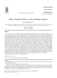
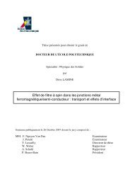
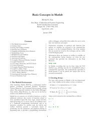
![[Diffusion-Limited Aggregation - A Model for Pattern Formation].](https://img.yumpu.com/52395246/1/190x245/diffusion-limited-aggregation-a-model-for-pattern-formation.jpg?quality=85)