The HLLC Riemann Solver

The HLLC Riemann SolverEleuterio TOROLaboratory of Applied MathematicsUniversity of Trento, Italytoro@ing.unitn.ithttp://www.ing.unitn.it/toroAugust 26, 2012

Abstract:This lecture is about a method to solve approximatelythe Riemann problem for the Euler equationsin order to derive a numerical flux for a conservative method:The HLLC Riemann solverREFERENCES:E F Toro, M Spruce and W Speares.Restoration of the contact surface in the HLL Riemann solver. Technical report CoA 9204. Department ofAerospace Science, College of Aeronautics, Cranfield Institute of Technology. UK. June, 1992.E F Toro, M Spruce and W Speares.Restoration of the contact surface in the Harten-Lax-van Leer Riemann solver. Shock Waves. Vol. 4, pages 25-34,1994.

Consider the general Initial Boundary Value Problem (IBVP)PDEs : U t + F(U) x = 0 , 0 ≤ x ≤ L , t > 0 ,ICs : U(x, 0) = U (0) (x) ,BCs : U(0, t) = U l (t) , U(L, t) = U r (t) ,with appropriate boundary conditions, as solved by the explicitconservative schemeU n+1i= U n i − ∆t∆x [F i+ 1 2The choice of numerical flux F i+12two classes of fluxes:⎫⎬⎭ (1)− F i−1 ] . (2)2determines the scheme. There◮ Upwind or Godunov-type fluxes (wave propagationinformation used explicitly) and◮ Centred or non-upwind (wave propagation information NOTused explicitly).

Godunov’s flux (Godunov 1959) isF i+12= F(U i+1 (0)) , (3)2in which U i+1 (0) is the exact similarity solution U2i+1 (x/t) of the2Riemann problem⎫U t + F(U)⎧ x = 0 ,⎪⎬⎨ U L if x < 0 ,(4)U(x, 0) =⎩⎪⎭U R if x > 0 ,evaluated at x/t = 0.

Example: 3D Euler equations.⎡ ⎤ ⎡ρρuU =⎢ ρv⎥⎣ ρw ⎦ , F = ⎢⎣Eρuρu 2 + pρuvρuwu(E + p)⎤⎥⎦ . (5)The piece–wise constant initial data, in terms of primitivevariables, is⎡ ⎤ ⎡ ⎤ρ Lρ Ru LW L =⎢ v L⎥⎣ w L⎦ , W u RR =⎢ v R⎥⎣ w R⎦ . (6)p Lp R

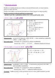
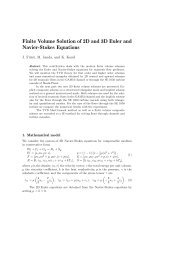
The Godunov flux F(U i+1 (0)) results from evaluation U2i+1 (x/t)2at x/t = 0, that is along the t–axis.(u-a)p*tu*(u,u,u)(u+a)ρuvwpLLLLLρvwρ*L *RL vRL0Fig. 1. Structure of the exact solution U i+1 (x/t) of the Riemann2problem for the x–split three dimensional Euler equations. Thereare five wave families associated with the eigenvaluesu − a, u (of multiplicity 3) and u + a.wRρuvwpRRRRRx

Integral RelationsConsider the control volume V = [x L , x R ] × [0, T ] depicted in Fig.2, withx L ≤ TS L , x R ≥ TS R , (7)S L and S R are the fastest signal velocities and T is a chosen time.The integral form of the conservation laws in (4) in V reads∫ xR∫ xR∫ T∫ TU(x, T )dx = U(x, 0)dx+ F(U(x L , t))dt− F(U(x R , t))dt .x L x L00(8)Evaluation of the right–hand side of this expression gives∫ xRU(x, T )dx = x R U R − x L U L + T (F L − F R ) , (9)x Lwhere F L = F(U L ) and F R = F(U R ).We call (9) the consistency condition.

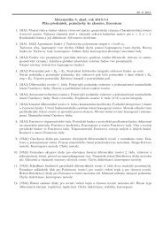
Now split left–hand side of (8) into three integrals, namely∫ xR∫ TSL∫ TSR∫ xRU(x, T )dx = U(x, T )dx + U(x, T )dx + U(x, T )dxx L x L TS L TS RSLtSRTxLTSLTSRFig. 2. Control volume [x L , x R ] × [0, T ] on x–t plane. S L and S R are thefastest signal velocities arising from the solution of the Riemann problem.xRx

Evaluate the first and third terms on the right–hand side to obtain∫ xR∫ TSRU(x, T )dx = U(x, T )dx+(TS L −x L )U L +(x R −TS R )U R .x L TS LComparing (10) with (9) gives(10)∫ TSRTS LU(x, T )dx = T (S R U R − S L U L + F L − F R ) . (11)On division through by the length T (S R − S L ), which is the widthof the wave system of the solution of the Riemann problembetween the slowest and fastest signals at time T , we have∫1 TSRU(x, T )dx = S RU R − S L U L + F L − F R. (12)T (S R − S L ) TS LS R − S L

Thus, the integral average of the exact solution of the Riemannproblem between the slowest and fastest signals at time T is aknown constant, provided that the signal speeds S L and S R areknown; such constant is the right–hand side of (12) and we denoteit byU hll = S RU R − S L U L + F L − F RS R − S L. (13)We now apply the integral form of the conservation laws to the leftportion of Fig. 10.2, that is the control volume [x L , 0] × [0, T ]. Weobtain∫ 0TS LU(x, T )dx = −TS L U L + T (F L − F 0L ) , (14)where F 0L is the flux F(U) along the t–axis. Solving for F 0L wefindF 0L = F L − S L U L − 1 T∫ 0TS LU(x, T )dx . (15)

Evaluation of the integral form of the conservation laws on thecontrol volume [0, x R ] × [0, T ] yieldsF 0R = F R − S R U R + 1 T∫ TSRThe reader can easily verify that the equalityF 0L = F 0R0U(x, T )dx . (16)results in the consistency condition (9). All relations so far areexact, as we are assuming the exact solution of the Riemannproblem.

The HLL flux F hll for the subsonic case S L ≤ 0 ≤ S R is found byinserting U hll in (13) into (15) or (16) to obtainorF hll = F L + S L (U hll − U L ) , (18)F hll = F R + S R (U hll − U R ) . (19)Use of (13) in (18) or (19) gives the HLL fluxF hll = S RF L − S L F R + S L S R (U R − U L )S R − S L(20)for the subsonic case S L ≤ 0 ≤ S R .

The corresponding HLL intercell flux for the approximate Godunovmethod is then given by⎧F L if 0 ≤ S L ,F hlli+ 1 2⎪⎨=⎪⎩S R F L − S L F R + S L S R (U R − U L )S R − S L, if S L ≤ 0 ≤ S R ,F R if 0 ≥ S R .(21)◮ Given the speeds S L and S R we have an approximate intercellflux (21) to be used in the conservative formula (2) toproduce an approximate Godunov method.◮ A shortcoming of the HLL scheme, with its two-wave model,is exposed by contact discontinuities, shear waves andmaterial interfaces, or any type of intermediate waves.

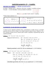
The HLLC Approximate Riemann Solver (Toro et al, 1992).◮ The HLLC scheme is a modification of the HLL schemewhereby the missing contact and shear waves in the Eulerequations are restored.◮ HLLC for the Euler equations has a three-wave modeltS L S*S RU * L U*RU L U R0Fig. 4. HLLC approximate Riemann solver. Solution in the StarRegion consists of two constant states separated from each otherby a middle wave of speed S ∗ .x

Useful Relations. Consider Fig. 2.◮ Evaluation of the integral form of the conservation laws in thecontrol volume reproduces the result of equation (12), even ifvariations of the integrand across the wave of speed S ∗ areallowed.◮ Note that the consistency condition (9) effectively becomesthe condition (12).◮ By splitting the left–hand side of integral (12) into two termswe obtain1T (S R − S L )∫ TSRTS LU(x, T )dx = U ∗L + U ∗R , (22)

where the following integral averages are introducedU ∗L =U ∗R =∫1 TS∗U(x, T )dx ,T (S ∗ − S L ) TS L∫1 TSRU(x, T )dx .T (S R − S ∗ ) TS ∗⎫⎪⎬⎪⎭(23)Use of (23) into (22) and use of (12), make condition (9)( ) ( )S∗ − SL SR − S ∗U ∗L +U ∗R = U hll , (24)S R − S L S R − S LThe HLLC approximate Riemann solver is given as follows⎧xU L , ift ⎪⎨≤ S L ,UŨ(x, t) = ∗L , if S L ≤ x t ≤ S ∗ ,U ⎪⎩ ∗R , if S ∗ ≤ x t ≤ S R ,xU R , ift ≥ S R .(25)

Now we seek a corresponding HLLC numerical flux of the form⎧F L , if 0 ≤ S L ,⎪⎨F hllc F= ∗L , if S L ≤ 0 ≤ S ∗ ,(26)i+ 1 2 F ⎪⎩ ∗R , if S ∗ ≤ 0 ≤ S R ,F R , if 0 ≥ S R ,with the intermediate fluxes F ∗L and F ∗R still to be determined, seeFig. 4. By integrating over appropriate control volumes we obtainF ∗L = F L + S L (U ∗L − U L ) , (27)F ∗R = F ∗L + S ∗ (U ∗R − U ∗L ) , (28)F ∗R = F R + S R (U ∗R − U R ) . (29)These are three equations for the four unknowns vectors U ∗L , F ∗L ,U ∗R , F ∗R .

We seek the solution for the two unknown intermediate fluxes F ∗Land F ∗R . There are more unknowns than equations and some extraconditions need to be imposed, in order to solve the algebraicproblem. We imposep ∗L = p ∗R = p ∗ ,u ∗L = u ∗R = u ∗ ,v ∗L = v L , v ∗R = v R ,w ∗L = w L , w ∗R = w R .}for pressure and normal velocity (30)}for tangential velocities(31)Conditions (30), (31) are identically satisfied by the exact solution.In addition we imposeS ∗ = u ∗ (32)and thus if an estimate for S ∗ is known, the normal velocitycomponent u ∗ in the Star Region is known.

Now equations (27) and (29) can be re–arranged asS L U ∗L − F ∗L = S L U L − F L , (33)S R U ∗R − F ∗R = S R U R − F R , (34)where the right–hand sides of (33) and (34) are known constantvectors (data). We also note the useful relationF(U) = uU + pD , D = [0, 1, 0, 0, u] T . (35)Assuming S L and S R to be known and performing algebraicmanipulations of the first and second components of equations(33)–(34) one obtainsp ∗L = p L +ρ L (S L −u L )(S ∗ −u L ) , p ∗R = p R +ρ R (S R −u R )(S ∗ −u R ) .(36)

From (30) p ∗L = p ∗R , which from (36) givesS ∗ = p R − p L + ρ L u L (S L − u L ) − ρ R u R (S R − u R )ρ L (S L − u L ) − ρ R (S R − u R ). (37)Manipulation of (33) and (34) and using p ∗L and p ∗R from (36)givesF ∗K = F K + S K (U ∗K − U K ) , (38)for K=L and K=R, with the intermediate states given as⎡1( )S ∗SK − u KU ∗K = ρ K v KS K − S ∗ ⎢[w K]⎣ E Kp K+ (S ∗ − u K ) S ∗ +ρ K ρ K (S K − u K )The final choice of the HLLC flux is made according to (26).⎤.⎥⎦(39)

Variation 1 of HLLC.From equations (33) and (34) we may write the following solutionsfor the state vectors U ∗L and U ∗RU ∗K = S K U K − F K + p ∗K D ∗S L − S ∗, D ∗ = [0, 1, 0, 0, S ∗ ] , (40)with p ∗L and p ∗R as given by (36). Substitution of p ∗K from (36)into (40) followed by use of (27) and (29) gives direct expressionsfor the intermediate fluxes asF ∗K = S ∗(S K U K − F K ) + S K (p K + ρ L (S K − u K )(S ∗ − u K ))D ∗,S K − S ∗(41)with the final choice of the HLLC flux made again according to(26).

Variation 2 of HLLC.A different HLLC flux is obtained by assuming a single meanpressure value in the Star Region, and given by the arithmeticaverage of the pressures in (36), namelyP LR = 1 2 [p L + p R + ρ L (S L − u L )(S ∗ − u L ) + ρ R (S R − u R )(S ∗ − u R )] .Then the intermediate state vectors are given by(42)U ∗K = S K U K − F K + P LR D ∗S K − S ∗. (43)Substitution of these into (27) and (29) gives the fluxes F ∗L andF ∗R asF ∗K = S ∗(S K U K − F K ) + S K P LR D ∗S K − S ∗. (44)Again the final choice of HLLC flux is made according to (26).

Remarks.◮ The original HLLC formulation (38)–(39) enforces thecondition p ∗L = p ∗R , which is satisfied by the exact solution.◮ In the alternative HLLC formulation (41) we relax suchcondition, being more consistent with the pressureapproximations (36).◮ There is limited practical experience with the alternativeHLLC formulations (41) and (44).◮ General equation of state. All manipulations, assuming thatwave speed estimates for S L and S R are available, are valid forany equation of state; this only enters when prescribingestimates for S L and S R .

Multidimensional multicomponent flow.Consider the advection of a chemical species of concentrations q lby the normal flow speed u. Then we can write the followingadvection equation∂ t q l + u∂ x q l = 0 , for l = 1, . . . , m .Note that these equations are written in non–conservative form.However, by combining these with the continuity equation weobtain a conservative form of these equations, namely(ρq l ) t + (ρuq l ) x = 0 , for l = 1, . . . , m .The eigenvalues of the enlarged system are as before, with theexception of λ 2 = u, which now, in three space dimensions, hasmultiplicity m + 3.

These conservation equations can then be added as newcomponents to the conservation equations in (1) or (4), with theenlarged vectors of conserved variables and fluxes given as⎡ ⎤ ⎡ρρuρvρwU =Eρq 1, F =. . .⎢ ρq l ⎥ ⎢⎣ . . . ⎦ ⎣ρq mρuρu 2 + pρuvρuwu(E + p)ρuq 1. . .ρuq l. . .ρuq m⎤. (45)⎥⎦

The HLLC flux accommodates these new equations in a verynatural way, and nothing special needs to be done. If the HLLCflux (38) is used, with F as in (45), then the intermediate statevectors are given by⎡⎤1S ∗v Kw K[]( )SK − u KE Kp KU ∗K = ρ K + (S ∗ − u K ) S ∗ +S K − S ∗ ρ K ρ K (S K − u K )(q 1 ) K. . .⎢(q l ) K⎥⎣. . .⎦(q m ) Kfor K = L and K = R..(46)

Wave Speed Estimates

We need estimates S L , S ∗ and S R . Davis (1988) suggestedS L = u L − a L , S R = u R + a R , (47)S L = min {u L − a L , u R − a R } , S R = max {u L + a L , u R + a R } .(48)Both Davis (1988) and Einfeldt (1988), proposedS L = ũ − ã , S R = ũ + ã , (49)ũ and ã are the Roe–average particle and sound speeds respectivelyũ =√ρL u L + √ [ρ R u R√ρL + √ , ã = (γ − 1)( ˜H − 1 1/2)] 2ũ2 , (50)ρ Rwith the enthalpy H = (E + p)/ρ approximated as˜H =√ρL H L + √ ρ R H R√ρL + √ ρ R. (51)

Einfeldt (1988) proposed the estimatesfor his HLLE solver, whereS L = ū − ¯d , S R = ū + ¯d , (52)¯d 2 =√ρL a 2 L + √ ρ R a 2 R√ρL + √ ρ R+ η 2 (u R − u L ) 2 (53)andη 2 = 1 √ √ρL ρR2 ( √ ρ L + √ ρ R ) 2 . (54)These wave speed estimates are reported to lead to effective androbust Godunov–type schemes.

One-wave model.Consider a one-wave model with single speed S + > 0.◮ Rusanov: By choosing S L = −S + and S R = S + in the HLLflux (20) one obtains a Rusanov flux (1961)F i+1/2 = 1 2 (F L + F R ) − 1 2 S + (U R − U L ) . (55)◮ Lax-Friedrichs: Another possibility is S + = S n max, the wavespeed for imposing the CFL condition, which satisfiesS n max = C cfl∆x∆t, (56)where C cfl is the CFL coefficient. For C cfl = 1, S + = ∆x∆t ,which gives the Lax–Friedrichs numerical fluxF i+1/2 = 1 2 (F L + F R ) − 1 ∆x2 ∆t (U R − U L ) . (57)

Pressure–Based Wave Speed EstimatesToro et al. (1994) suggested to first find an estimate p ∗ for thepressure in the Star Region and then take⎧⎨q K =⎩S L = u L − a L q L , S R = u R + a R q R , (58)[1 + γ + 12γ (p ∗/p K − 1)1 if p ∗ ≤ p K] 1/2if p ∗ > p K .◮ This choice discriminates between shocks and rarefactions.(59)◮ If the K wave is a rarefaction then the speed S K is the speedof the head of the rarefaction, the fastest signal.◮ If the K wave is a shock wave then the speed is anapproximation of the shock speed.

A simple, acoustic type approximation for pressure is (Toro, 1991)p ∗ = max(0, p pvrs ) , p pvrs = 1 2 (p L + p R ) − 1 2 (u R − u L )¯ρā , (60)where¯ρ = 1 2 (ρ L + ρ R ) , ā = 1 2 (a L + a R ) . (61)Another choice is furnished by the Two–Rarefaction Riemannsolver, namely[aL + a R − γ−12p ∗ = p tr =(u ] 1/zR − u L )a L /pL z + a R/pRz , (62)whereP LR =( ) z pL; z = γ − 1 . (63)p R 2γ

The Two–Shock Riemann solver givesp ∗ = p ts = g L(p 0 )p L + g R (p 0 )p R − ∆ug L (p 0 ) + g R (p 0 ), (64)whereg K (p) =for K = L and K = R.[AKp + B K] 1/2, p 0 = max(0, p pvrs ) , (65)

Summary of HLLC Fluxes◮ Step I: pressure estimate p ∗ .◮ Step II: wave speed estimates:with⎧⎨q K =⎩andS L = u L − a L q L , S R = u R + a R q R , (66)[1 + γ + 12γ (p ∗/p K − 1)1 if p ∗ ≤ p K] 1/2if p ∗ > p K .S ∗ = p R − p L + ρ L u L (S L − u L ) − ρ R u R (S R − u R )ρ L (S L − u L ) − ρ R (S R − u R )(67). (68)◮ Step III: HLLC flux. Compute the HLLC flux, according to⎧F L if 0 ≤ S L ,⎪⎨F hllc F= ∗L if S L ≤ 0 ≤ S ∗ ,(69)i+ 1 2 F ⎪⎩ ∗R if S ∗ ≤ 0 ≤ S R ,F R if 0 ≥ S R ,

F ∗K = F K + S K (U ∗K − U K ) (70)and⎡( )SK − u KU ∗K = ρ K S K − S ∗ ⎢⎣E Kρ K+ (S ∗ − u K )1S ∗v Kw K[S ∗ +p K]⎤⎥⎦ρ K (S K − u K )(71).

There are two variants of the HLLC flux in the third step, as seenbelow.◮ Step III: HLLC flux, Variant 1. Compute the numerical fluxesasF ∗K = S ∗(S K U K − F K ) + S K (p K + ρ L (S K − u K )(S ∗ − u K ))D ∗S K − S ∗,D ∗ = [0, 1, 0, 0, S ∗ ] T ,(72)and the final HLLC flux chosen according to (69).◮ Step III: HLLC flux, Variant 2. Compute the numerical fluxesasF ∗K = S ∗(S K U K − F K ) + S K P LR D ∗, (73)S K − S ∗with D ∗ as in (72) andP LR = 1 2 [p L+p R +ρ L (S L −u L )(S ∗ −u L )+ρ R (S R −u R )(S ∗ −u R )] .The final HLLC flux is chosen according to (69).(74)⎫⎪⎬⎪⎭

Numerical Results

Test problems:Test ρ L u L p L ρ R u R p R1 1.0 0.75 1.0 0.125 0.0 0.12 1.0 -2.0 0.4 1.0 2.0 0.43 1.0 0.0 1000.0 1.0 0.0 0.014 5.99924 19.5975 460.894 5.99242 -6.19633 46.09505 1.0 -19.59745 1000.0 1.0 -19.59745 0.016 1.4 0.0 1.0 1.0 0.0 1.07 1.4 0.1 1.0 1.0 0.1 1.0Table 1. Data for seven test problems with exact solution

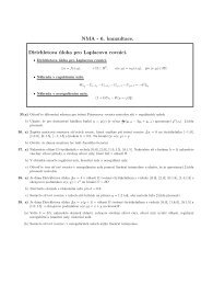
11.6Density0.5Velocity0.800 0.5 1Position00 0.5 1Position13.8Pressure0.5Internal energy00 0.5 1Position1.80 0.5 1PositionGodunov’s method with HLLC Riemann solver applied to Test 1,with x 0 = 0.3. Numerical (symbol) and exact (line) solutions arecompared at time 0.2.

12Density0.5Velocity000 0.5 1Position-20 0.5 1Position0.5Pressure0.2500 0.5 1PositionInternal energy10.500 0.5 1PositionGodunov’s method with HLLC Riemann solver applied to Test 2,with x 0 = 0.5. Numerical (symbol) and exact (line) solutions arecompared at time 0.15.

256Density3Velocity12.5000 0.5 1Position0 0.5 1Position10002500Pressure500Internal energy125000 0.5 1Position00 0.5 1PositionGodunov’s method with HLLC Riemann solver applied to Test 3,with x 0 = 0.5. Numerical (symbol) and exact (line) solutions arecompared at time 0.012.

3020Density15Velocity10000 0.5 1Position-100 0.5 1Position1800300Pressure900Internal energy15000 0.5 1Position00 0.5 1PositionGodunov’s method with HLLC Riemann solver applied to Test 4,with x 0 = 0.4. Numerical (symbol) and exact (line) solutions arecompared at time 0.035.

560Density3Velocity-2000 0.5 1Position0 0.5 1Position10002500Pressure500Internal energy125000 0.5 1Position00 0.5 1PositionGodunov’s method with HLLC Riemann solver applied to Test 5,with x 0 = 0.8. Numerical (symbol) and exact (line) solutions arecompared at time 0.012.

560Density3Velocity-2000 0.5 1Position0 0.5 1Position10002500Pressure500Internal energy125000 0.5 1Position00 0.5 1PositionGodunov’s method with HLL Riemann solver applied to Test 5,with x 0 = 0.8. Numerical (symbol) and exact (line) solutions arecompared at time 0.012.

HLL density1.41HLLC density1.410 0.5 1position0 0.5 1positionHLL density1.41HLLC density1.410 0.5 1position0 0.5 1positionGodunov’s method with HLL (left) and HLLC (right) Riemannsolvers applied to Tests 6 and 7. Numerical (symbol) and exact(line) solutions are compared at time 2.0.

Closing Remarks:

◮ We have presented HLLC for the Euler equations.◮ For the 2D shallow water equations see Toro E F Shockcapturing methods for free-surface shallow flows. Wiley andSons, 2001.◮ For Turbulent flow applications (implicit version of HLLC), seeBatten, Leschziner and Goldberg (1997).◮ For extensions to MHD equations see Gurski (2004), Li(2005), Mignone et al. (2006++).◮ For application to two-phase flow see Tokareva and Toro, JCP(2010).◮ For extensions see Takahiro (2005) and Bouchut (2007),Mignone (2005).