bundle block adjustment with 3d natural cubic splines
bundle block adjustment with 3d natural cubic splines bundle block adjustment with 3d natural cubic splines
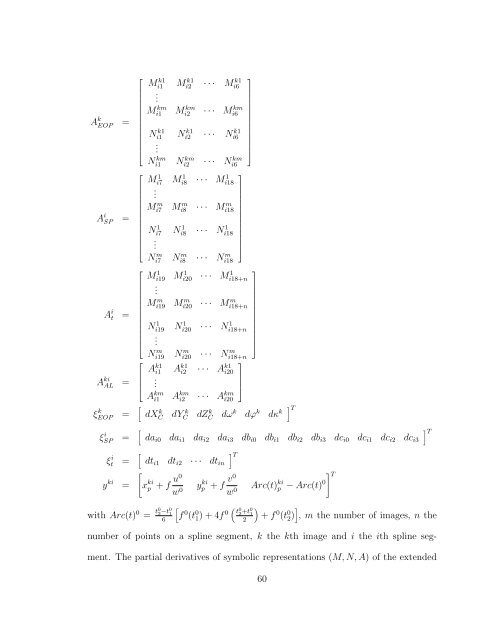
A k EOP =A i SP =A i t =A kiAL =⎡⎢⎣M k1i1.M kmi1N k1i1.N kmi1Mi2 k1 · · · Mi6k1Mi2 km · · · Mi6kmNi2 k1 · · · Ni6k1Ni2 km · · · Ni6km⎤⎡Mi7 1 Mi8 1 · · · Mi181 .M i7 m Mi8 m · · · Mi18m N i7 1 Ni8 1 · · · Ni181⎢⎣.Ni7 m Ni8 m · · · Ni18m⎥⎦⎡Mi19 1 Mi20 1 · · · Mi18+n1 .M i19 m Mi20 m · · · Mi18+nm N i19 1 Ni20 1 · · · Ni18+n1⎢⎣ .Ni19 m Ni20 m · · · Ni18+nm ⎡⎤⎢⎣A k1i1.A kmi1A k1i2 · · · A k1i20A kmi2 · · · A kmi20ξ k EOP = [ dX k C dY k C dZ k C dω k dϕ k dκ k ] T⎥⎦⎤⎥⎦⎤⎥⎦ξ i SP = [ da i0 da i1 da i2 da i3 db i0 db i1 db i2 db i3 dc i0 dc i1 dc i2 dc i3] Tξ i t = [ dt i1 dt i2 · · · dt in] Ty ki =[x kip+ f u0w 0y kip+ f v0w 0Arc(t) kip− Arc(t) 0 ] Twith Arc(t) 0 = t0 2 −t0 16[f 0 (t 0 1) + 4f ( ) 0 t 0 2 +t0 12 + f 0 (t 0 2) ] , m the number of images, n thenumber of points on a spline segment, k the kth image and i the ith spline segment.The partial derivatives of symbolic representations (M, N, A) of the extended60
collinearity model are described in appendix A. Since the equation system of theintegrated model has datum defects of seven, the control information about the coordinatesystem is required to obtain the seven transformation parameters. In a generalphotogrammetric network, the rank deficiency referred as datum defects is seven.Estimates of the unknown parameters are obtained by the least squares solutionwhich minimizes the sum of squared deviations. A non-linear least squares system isrequired in the conventional non-linear photogrammetric solution to obtain orientationparameters. Many observations in photogrammetry are random variables whichare considered as different values in the case of repeated observations such as imagecoordinates of points on images. Each measured observation represents an estimateof random variables of the image coordinates of points on images. If image coordinatesof points are measured using the digital photogrammetric workstation, thevalues would be measured slightly differently for each measurement. The integratedand linearized Gauss-Markov model and the least squares estimated parameter vectorwith its dispersion matrix arey ki = A IM ξ IM + e⎡A k EOP A i SP A i ⎤t⎢⎥A IM = ⎣⎦A kiALξ IM = [ ] TξEOP k ξSP i ξti (4.3)ˆξ IM = (A T IMP A IM ) −1 A T IMP y kiD(ˆξ IM ) = σ 2 o(A T IMP A IM ) −1with e˜N(0, σoP 2 −1 ) the error vector with zero mean and cofactor matrix P −1 , andvariance component σo 2 which can be known or not, ˆξ IM the least squares estimatedparameter vector and D(ˆξ IM ) the dispersion matrix.61
- Page 21 and 22: • Bundle block adjustment by the
- Page 23 and 24: Hessian. Interest point operators w
- Page 25 and 26: [60], Ebner and Ohlhof(1994) [16],
- Page 27 and 28: a complicated problem. The developm
- Page 29 and 30: ⎡⎢⎣x i − x py i − y p−f
- Page 31 and 32: x p = −f (X A + t · a − X C )r
- Page 33 and 34: surfaces and terrain models in 2D a
- Page 35 and 36: f(u) − e(u) = g(u)f(u) − e(u) =
- Page 37 and 38: Tankovich[69] used linear features
- Page 39 and 40: (a) 0th order continuity (b) 1st or
- Page 41 and 42: Cardinal splineA Cardinal spline is
- Page 43 and 44: 2.3.2 Fourier transformFourier seri
- Page 45 and 46: For other polyline expressions, Aya
- Page 47 and 48: Each segment of a natural cubic spl
- Page 49 and 50: ⎡⎢⎣2 11 4 11 4 1· · ·1 4 1
- Page 51 and 52: 3.2 Extended collinearity equation
- Page 53 and 54: R −1 = R T . The matrix R T (= R
- Page 55 and 56: dx p = M 1 dX C + M 2 dY C + M 3 dZ
- Page 57 and 58: In this research, the arc-length pa
- Page 59 and 60: =√∫ √√√ ()ti+1−f u′ (
- Page 61 and 62: This equation can be replaced with
- Page 63 and 64: order polynomial using Newton’s d
- Page 65 and 66: y collinearity equations, tangents
- Page 67 and 68: d tan(θ t ) = w′ (v ′ w − w
- Page 69 and 70: y each two points, which are four e
- Page 71: +M 14 db i3 + M 15 dc i0 + M 16 dc
- Page 75 and 76: [ ] [ ] [ ]N11 N 12 ˆξ1 c1N12T =N
- Page 77 and 78: systematic errors in the image spac
- Page 79 and 80: interval based on the normal distri
- Page 81 and 82: 1 ∂Φ2 ∂l= (X C + d 1 l − a i
- Page 83 and 84: about splines, their relationships,
- Page 85 and 86: cubic spline in the image and the o
- Page 87 and 88: The redundancy budget of a tie poin
- Page 89 and 90: of bundle block adjustment is requi
- Page 91 and 92: ξ kiSP = [ da i0 da i1 da i2 da i3
- Page 93 and 94: Spline location parametersImage 1 I
- Page 95 and 96: Spline location parametersImage 1 I
- Page 97 and 98: 5.3 Recovery of EOPs and spline par
- Page 99 and 100: Table 5.7 expressed the convergence
- Page 101 and 102: Iteration with an incorrect spline
- Page 103 and 104: Vertical aerial photographData 9 Ju
- Page 105 and 106: All locations are assumed as on the
- Page 107 and 108: of the Gauss-Markov model correspon
- Page 109 and 110: estimation is obstacled by the corr
- Page 111 and 112: Interior orientation defines a tran
- Page 113 and 114: + fu ( w2 31 (X i (t) − X C ) + s
- Page 115 and 116: A.2 Derivation of arc-length parame
- Page 117 and 118: +2f( t [1 + t 2) − 1 22s 12 (Y i
- Page 119 and 120: +Du ′ ( t 1 + t 22)2r 11 t + Dv
- Page 121 and 122: A 17 = t [2 − t 1 16 2 f(t 1) −
A k EOP =A i SP =A i t =A kiAL =⎡⎢⎣M k1i1.M kmi1N k1i1.N kmi1Mi2 k1 · · · Mi6k1Mi2 km · · · Mi6kmNi2 k1 · · · Ni6k1Ni2 km · · · Ni6km⎤⎡Mi7 1 Mi8 1 · · · Mi181 .M i7 m Mi8 m · · · Mi18m N i7 1 Ni8 1 · · · Ni181⎢⎣.Ni7 m Ni8 m · · · Ni18m⎥⎦⎡Mi19 1 Mi20 1 · · · Mi18+n1 .M i19 m Mi20 m · · · Mi18+nm N i19 1 Ni20 1 · · · Ni18+n1⎢⎣ .Ni19 m Ni20 m · · · Ni18+nm ⎡⎤⎢⎣A k1i1.A kmi1A k1i2 · · · A k1i20A kmi2 · · · A kmi20ξ k EOP = [ dX k C dY k C dZ k C dω k dϕ k dκ k ] T⎥⎦⎤⎥⎦⎤⎥⎦ξ i SP = [ da i0 da i1 da i2 da i3 db i0 db i1 db i2 db i3 dc i0 dc i1 dc i2 dc i3] Tξ i t = [ dt i1 dt i2 · · · dt in] Ty ki =[x kip+ f u0w 0y kip+ f v0w 0Arc(t) kip− Arc(t) 0 ] T<strong>with</strong> Arc(t) 0 = t0 2 −t0 16[f 0 (t 0 1) + 4f ( ) 0 t 0 2 +t0 12 + f 0 (t 0 2) ] , m the number of images, n thenumber of points on a spline segment, k the kth image and i the ith spline segment.The partial derivatives of symbolic representations (M, N, A) of the extended60


