bundle block adjustment with 3d natural cubic splines

Recommendations

Info

In the case of straight lines and conic sections, tangents are the additional observationsin the integrated model. Conic sections which, like points, are good mathematicalconstraints since conic sections are non-singular curves of degree 2. Second-degreeequations provide the information for reconstruction and transformation and conicsections are divided by the eccentricity e as shown in table 4.1. Since conic sectionscan adopt more constraints than points and straight line features, conic sections areuseful for close range photogrammetric applications. In addition, conic sections havethe strength in the correspondence establishment between 3D conic sections in theobject space and their counterpart features in the 2D projected image space.Eccentricity Conic forme=0 Circle0 < e < 1 Ellipsee = 1 Parabolae > 1 HyperbolaTable 4.1: Relationship between the eccentricity and the conic formJi et al.(2000) [36] employed conic sections for the recovery of EOPs andHeikkila(2000) [33] used them for camera calibration. Hough transformation reducesthe time complexity of the conic section extraction using five parameter spaces for asingle-photo resection, camera calibration and triangulation [63].x p + f u0w 0 = M 1 dX C + M 2 dY C + M 3 dZ C + M 4 dω + M 5 dϕ + M 6 dκ + M 7 da i0+M 8 da i1 + M 9 da i2 + M 10 da i3 + M 11 db i0 + M 12 db i1 + M 13 db i258
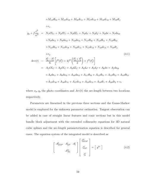
+M 14 db i3 + M 15 dc i0 + M 16 dc i1 + M 17 dc i2 + M 18 dc i3 + M 19 dt j+e xy p + f v0w 0 = N 1 dX C + N 2 dY C + N 3 dZ C + N 4 dω + N 5 dϕ + N 6 dκ + N 7 da i0+N 8 da i1 + N 9 da i2 + N 10 da i3 + N 11 db i0 + N 12 db i1 + N 13 db i2Arc(t) − t0 2 − t 0 16+N 14 db i3 + N 15 dc i0 + N 16 dc i1 + N 17 dc i2 + N 18 dc i3 + N 19 dt j+e y (4.1)[) ]f 0 (t 0 1) + 4f 0 ( t02 + t 0 12+ f 0 (t 0 2)= A 1 dX C + A 2 dY C + A 3 dZ C + A 4 dω + A 5 dϕ + A 6 dκ + A 7 da i0+A 8 da i1 + A 9 da i2 + A 10 da i3 + A 11 db i0 + A 12 db i1 + A 13 db i2 + A 14 db i3+A 15 dc i0 + A 16 dc i1 + A 17 dc i2 + A 18 dc i3 + A 19 dt 1 + A 20 dt 2 + e twhere x p , y p the photo coordinates and Arc(t) the arc-length between two locationsrespectively.Parameters are linearized in the previous three sections and the Gauss-Markovmodel is employed for the unknown parameter estimation. Tangent observation canbe added in case of straight linear features and conic sections but in this modelbundle block adjustment with the extended collinearity equations for 3D naturalcubic splines and the arc-length parameterization equation is described for generalcases. The equation system of the integrated model is described as⎡⎢⎣A k EOP A i SP A i tA kiAL⎡ξ⎤ EOPk ⎥⎦ξSPi ⎢⎣ξti⎤= [ y ] ki (4.2)⎥⎦59
Page 2:
c○ Copyright byWon Hee Lee2008
Page 7 and 8:
ACKNOWLEDGMENTSThanks be to God, my
Page 10 and 11:
3. BUNDLE BLOCK ADJUSTMENTWITH 3D N
Page 13 and 14:
CHAPTER 1INTRODUCTION1.1 OverviewOn
Page 15 and 16:
y an intersection employing more th
Page 17 and 18:
similarity of geometric properties
Page 19 and 20: straight linear features or formula
Page 21 and 22: • Bundle block adjustment by the
Page 23 and 24: Hessian. Interest point operators w
Page 25 and 26: [60], Ebner and Ohlhof(1994) [16],
Page 27 and 28: a complicated problem. The developm
Page 29 and 30: ⎡⎢⎣x i − x py i − y p−f
Page 31 and 32: x p = −f (X A + t · a − X C )r
Page 33 and 34: surfaces and terrain models in 2D a
Page 35 and 36: f(u) − e(u) = g(u)f(u) − e(u) =
Page 37 and 38: Tankovich[69] used linear features
Page 39 and 40: (a) 0th order continuity (b) 1st or
Page 41 and 42: Cardinal splineA Cardinal spline is
Page 43 and 44: 2.3.2 Fourier transformFourier seri
Page 45 and 46: For other polyline expressions, Aya
Page 47 and 48: Each segment of a natural cubic spl
Page 49 and 50: ⎡⎢⎣2 11 4 11 4 1· · ·1 4 1
Page 51 and 52: 3.2 Extended collinearity equation
Page 53 and 54: R −1 = R T . The matrix R T (= R
Page 55 and 56: dx p = M 1 dX C + M 2 dY C + M 3 dZ
Page 57 and 58: In this research, the arc-length pa
Page 59 and 60: =√∫ √√√ ()ti+1−f u′ (
Page 61 and 62: This equation can be replaced with
Page 63 and 64: order polynomial using Newton’s d
Page 65 and 66: y collinearity equations, tangents
Page 67 and 68: d tan(θ t ) = w′ (v ′ w − w
Page 69: y each two points, which are four e
Page 73 and 74: collinearity model are described in
Page 75 and 76: [ ] [ ] [ ]N11 N 12 ˆξ1 c1N12T =N
Page 77 and 78: systematic errors in the image spac
Page 79 and 80: interval based on the normal distri
Page 81 and 82: 1 ∂Φ2 ∂l= (X C + d 1 l − a i
Page 83 and 84: about splines, their relationships,
Page 85 and 86: cubic spline in the image and the o
Page 87 and 88: The redundancy budget of a tie poin
Page 89 and 90: of bundle block adjustment is requi
Page 91 and 92: ξ kiSP = [ da i0 da i1 da i2 da i3
Page 93 and 94: Spline location parametersImage 1 I
Page 95 and 96: Spline location parametersImage 1 I
Page 97 and 98: 5.3 Recovery of EOPs and spline par
Page 99 and 100: Table 5.7 expressed the convergence
Page 101 and 102: Iteration with an incorrect spline
Page 103 and 104: Vertical aerial photographData 9 Ju
Page 105 and 106: All locations are assumed as on the
Page 107 and 108: of the Gauss-Markov model correspon
Page 109 and 110: estimation is obstacled by the corr
Page 111 and 112: Interior orientation defines a tran
Page 113 and 114: + fu ( w2 31 (X i (t) − X C ) + s
Page 115 and 116: A.2 Derivation of arc-length parame
Page 117 and 118: +2f( t [1 + t 2) − 1 22s 12 (Y i
Page 119 and 120: +Du ′ ( t 1 + t 22)2r 11 t + Dv
Page 121 and 122:
A 17 = t [2 − t 1 16 2 f(t 1) −
Page 123 and 124:
1−u ′ w − w ′ u {w′ [s 21
Page 125 and 126:
BIBLIOGRAPHY[1] Ackerman, F., and V
Page 127 and 128:
[24] Haala, N., and G. Vosselman. 1
Page 129 and 130:
[49] Parian, J.A., and A. Gruen. 20
Page 131:
[73] Vosselman, G., and H. Veldhuis
show all

bundle block adjustment with 3d natural cubic splines

Create successful ePaper yourself

Delete template?

Save as template?