bundle block adjustment with 3d natural cubic splines
bundle block adjustment with 3d natural cubic splines bundle block adjustment with 3d natural cubic splines
= A 1 dX C + A 2 dY C + A 3 dZ C + A 4 dω + A 5 dϕ + A 6 dκ + A 7 da 0+A 8 da 1 + A 9 da 2 + A 10 da 3 + A 11 db 0 + A 12 db 1 + A 13 db 2 + A 14 db 3+A 15 dc 0 + A 16 dc 1 + A 17 dc 2 + A 18 dc 3 + A 19 dt 1 + A 20 dt 2 + e awith t 0 1, t 0 2, f(t 0 ) the approximate parameters by (XC, 0 YC, 0 ZC, 0 ω 0 , ϕ 0 , κ 0 , a 0 0, a 0 1, a 0 2,a 0 3, b 0 0, b 0 1, b 0 2, b 0 3, c 0 0, c 0 1, c 0 2, c 0 3, t 0 i ) and e a the stochastic error of the arc-length betweentwo locations with zero expectation. A 1 , · · · , A 20 denote the partial derivatives of thearc-length parameterization of a 3D natural cubic spline. Detailed derivations are inAppendix A.2.3.4 Tangents of spline between image and object spaceSince employing spline leads to over parameterization, geometric constraints arerequired to solve the system, such as slope, distance, perpendicularity, coplanar features.While some of the geometric constraints, slope and distance observations, aredependent on splines, other constraints increase non-redundant information in adjustmentto reduce the overall rank deficiency of the system. Tangents of splines provideadditional constraints to solve the over parameterization of 3D natural cubic splines.In case linear features in the object space are straight lines or conic sections. Tangentsare one of straight line constraints incorporated into bundle block adjustment usingthe assumption that the transformation of straight lines in the object space is straightlines as well in the image space. In linear features using collinearity equations, therelationship establishment of two corresponding properties in the image space andthe object space is possible. Since tangents are independent measurements in theimage space and the object space and the relationship between them is established52
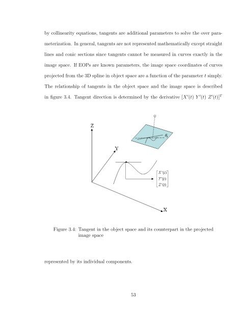
y collinearity equations, tangents are additional parameters to solve the over parameterization.In general, tangents are not represented mathematically except straightlines and conic sections since tangents cannot be measured in curves exactly in theimage space. If EOPs are known parameters, the image space coordinates of curvesprojected from the 3D spline in object space are a function of the parameter t simply.The relationship of tangents in the object space and the image space is describedin figure 3.4. Tangent direction is determined by the derivative [X ′ (t) Y ′ (t) Z ′ (t)] TFigure 3.4: Tangent in the object space and its counterpart in the projectedimage spacerepresented by its individual components.53
- Page 13 and 14: CHAPTER 1INTRODUCTION1.1 OverviewOn
- Page 15 and 16: y an intersection employing more th
- Page 17 and 18: similarity of geometric properties
- Page 19 and 20: straight linear features or formula
- Page 21 and 22: • Bundle block adjustment by the
- Page 23 and 24: Hessian. Interest point operators w
- Page 25 and 26: [60], Ebner and Ohlhof(1994) [16],
- Page 27 and 28: a complicated problem. The developm
- Page 29 and 30: ⎡⎢⎣x i − x py i − y p−f
- Page 31 and 32: x p = −f (X A + t · a − X C )r
- Page 33 and 34: surfaces and terrain models in 2D a
- Page 35 and 36: f(u) − e(u) = g(u)f(u) − e(u) =
- Page 37 and 38: Tankovich[69] used linear features
- Page 39 and 40: (a) 0th order continuity (b) 1st or
- Page 41 and 42: Cardinal splineA Cardinal spline is
- Page 43 and 44: 2.3.2 Fourier transformFourier seri
- Page 45 and 46: For other polyline expressions, Aya
- Page 47 and 48: Each segment of a natural cubic spl
- Page 49 and 50: ⎡⎢⎣2 11 4 11 4 1· · ·1 4 1
- Page 51 and 52: 3.2 Extended collinearity equation
- Page 53 and 54: R −1 = R T . The matrix R T (= R
- Page 55 and 56: dx p = M 1 dX C + M 2 dY C + M 3 dZ
- Page 57 and 58: In this research, the arc-length pa
- Page 59 and 60: =√∫ √√√ ()ti+1−f u′ (
- Page 61 and 62: This equation can be replaced with
- Page 63: order polynomial using Newton’s d
- Page 67 and 68: d tan(θ t ) = w′ (v ′ w − w
- Page 69 and 70: y each two points, which are four e
- Page 71 and 72: +M 14 db i3 + M 15 dc i0 + M 16 dc
- Page 73 and 74: collinearity model are described in
- Page 75 and 76: [ ] [ ] [ ]N11 N 12 ˆξ1 c1N12T =N
- Page 77 and 78: systematic errors in the image spac
- Page 79 and 80: interval based on the normal distri
- Page 81 and 82: 1 ∂Φ2 ∂l= (X C + d 1 l − a i
- Page 83 and 84: about splines, their relationships,
- Page 85 and 86: cubic spline in the image and the o
- Page 87 and 88: The redundancy budget of a tie poin
- Page 89 and 90: of bundle block adjustment is requi
- Page 91 and 92: ξ kiSP = [ da i0 da i1 da i2 da i3
- Page 93 and 94: Spline location parametersImage 1 I
- Page 95 and 96: Spline location parametersImage 1 I
- Page 97 and 98: 5.3 Recovery of EOPs and spline par
- Page 99 and 100: Table 5.7 expressed the convergence
- Page 101 and 102: Iteration with an incorrect spline
- Page 103 and 104: Vertical aerial photographData 9 Ju
- Page 105 and 106: All locations are assumed as on the
- Page 107 and 108: of the Gauss-Markov model correspon
- Page 109 and 110: estimation is obstacled by the corr
- Page 111 and 112: Interior orientation defines a tran
- Page 113 and 114: + fu ( w2 31 (X i (t) − X C ) + s
y collinearity equations, tangents are additional parameters to solve the over parameterization.In general, tangents are not represented mathematically except straightlines and conic sections since tangents cannot be measured in curves exactly in theimage space. If EOPs are known parameters, the image space coordinates of curvesprojected from the 3D spline in object space are a function of the parameter t simply.The relationship of tangents in the object space and the image space is describedin figure 3.4. Tangent direction is determined by the derivative [X ′ (t) Y ′ (t) Z ′ (t)] TFigure 3.4: Tangent in the object space and its counterpart in the projectedimage spacerepresented by its individual components.53


