bundle block adjustment with 3d natural cubic splines

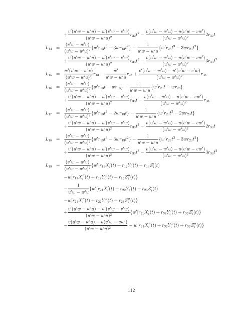
+ v′ (u ′ w − w ′ u) − u ′ (v ′ w − v ′ w)r(u ′ w − w ′ u) 2 32 t 2 − v(u′ w − w ′ u) − u(v ′ w − vw ′ )2r(u ′ w − w ′ u) 2 32 tL 14 = (v′ w − w ′ v)(u ′ w − w ′ u) 2 {w′ r 13 t 3 − 3wr 13 t 2 1} −u ′ w − w ′ u {w′ r 23 t 3 − 3wr 23 t 2 }+ v′ (u ′ w − w ′ u) − u ′ (v ′ w − v ′ w)r(u ′ w − w ′ u) 2 33 t 3 − v(u′ w − w ′ u) − u(v ′ w − vw ′ )3r(u ′ w − w ′ u) 2 33 t 2L 15 = w′ (v ′ w − w ′ v)(u ′ w − w ′ u) r w ′2 13 −u ′ w − w ′ u r 23 + v′ (u ′ w − w ′ u) − u ′ (v ′ w − v ′ w)r(u ′ w − w ′ u) 2 33L 16 = (v′ w − w ′ v)1(u ′ w − w ′ u) 2 {w′ r 13 t − wr 13 } −u ′ w − w ′ u {w′ r 23 t − wr 23 }+ v′ (u ′ w − w ′ u) − u ′ (v ′ w − v ′ w)r(u ′ w − w ′ u) 2 33 t − v(u′ w − w ′ u) − u(v ′ w − vw ′ )r(u ′ w − w ′ u) 2 33L 17 = (v′ w − w ′ v)(u ′ w − w ′ u) 2 {w′ r 13 t 2 1− 2wr 13 t} −u ′ w − w ′ u {w′ r 23 t 2 − 2wr 23 t}+ v′ (u ′ w − w ′ u) − u ′ (v ′ w − v ′ w)r(u ′ w − w ′ u) 2 33 t 2 − v(u′ w − w ′ u) − u(v ′ w − vw ′ )2r(u ′ w − w ′ u) 2 33 tL 18 = (v′ w − w ′ v)(u ′ w − w ′ u) 2 {w′ r 13 t 3 − 3wr 13 t 2 1} −u ′ w − w ′ u {w′ r 23 t 3 − 3wr 23 t 2 }+ v′ (u ′ w − w ′ u) − u ′ (v ′ w − v ′ w)(u ′ w − w ′ u) 2 r 33 t 3 − v(u′ w − w ′ u) − u(v ′ w − vw ′ )(u ′ w − w ′ u) 2 3r 33 t 2L 19 = (v′ w − w ′ v)(u ′ w − w ′ u) 2 {w′ [r 11 X ′ i(t) + r 12 Y ′i (t) + r 13 Z ′ i(t)−w[r 11 X ′′i (t) + r 12 Y ′′i (t) + r 13 Z ′′i (t)}1−u ′ w − w ′ u {w′ [r 21 X i(t) ′ + r 22 Y i ′ (t) + r 23 Z i(t)′−w[r 21 X ′′i (t) + r 22 Y ′′i (t) + r 23 Z ′′i (t)}+ v′ (u ′ w − w ′ u) − u ′ (v ′ w − v ′ w)(u ′ w − w ′ u) 2 {w ′ [r 31 X ′ i(t) + r 32 Y ′i (t) + r 33 Z ′ i(t)}− v(u′ w − w ′ u) − u(v ′ w − vw ′ )(u ′ w − w ′ u) 2 − w[r 31 X ′′i (t) + r 32 Y ′′i (t) + r 33 Z ′′i (t)}112