introduction to Mathematica - Mathematics

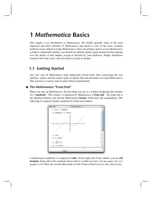
Mathematica Basics 3‡ The Documentation CenterMathematica’s Documentation Center may be accessed by selecting Documentation Centerfrom the Help menu. Among the wealth of information available through the DocumentationCenter are descriptions of all of Mathematica’s built-in functions, including examplesof their use and links to related tutorials. You can also enter commands from within theDocumentation Center. (Whatever you change there will not be saved.)The Documentation Center provides a great deal of tutorial material. If you’re a beginner,we suggest that you peruse the tutorials found by entering each of the following in theDocumentation Center search field.tutorial/UsingTheMathematicaSystemOverviewtutorial/InputAndOutputInNotebooksOverviewtutorial/BuildingUpCalculationsOverviewtutorial/EnteringTwoDimensionalExpressionsOverviewtutorial/GraphicsAndSoundOverview(Hopefully future updates to the Documentation Center will provide a more convenient wayto access these and other tutorials.)

Mathematica Basics 5‡ Parentheses, Brackets, and BracesThe syntax of Mathematica is absolutely strict and consistent (and quite simple once you getused to it). For that reason, there are some differences between Mathematica’s syntax andthe often inconsistent and sometimes ambiguous mathematical notation that we’re all usedto. For example:Parentheses are used only for grouping expressions.x Hx + 2L 2x H2 + xL 2Brackets are used only to enclose the argument(s) of a function.Cos@p ê 3D12Braces are used only to enclosed the elements of a list (which might represent a set, anordered pair, or even a matrix).81, 2, 3, 4

6 Chapter 1One way to obtain a numerical result is to use the numerical evaluation function, N.NA123 ë768 E4.43838We also get a numerical result if any of the numbers in the expression are made numericalby use of a decimal point.123. í 7684.43838Unless we cause a numerical result, Mathematica typically returns an exact form, which inmany cases is identical to the expression entered.CosB p 12 F1 + 32 2Log@2DLog@2D‡ Names and Capitalization; Basic FunctionsAll built-in Mathematica objects~functions, constants, options, etc.~have full names thatbegin with a capital letter (or in the case of certain “global” parameters, a dollar signfollowed by a capital letter).Sin@p ê 3D32PrimeQ@22 801 763 489DTrueSolveAx 2 + x - 12 ã 0, xE88x Ø -4

Mathematica Basics 9Notice that the following plot chops off high and low parts of the curve.PlotB SinA2 x2 E, 8x, 0, 10

10 Chapter 1To plot more than one function at once, we give Plot a list of functions.PlotA9x ‰ -xê2 Cos@p xD, x ‰ -xê2 Sin@p xD=, 8x, 0, 12

Mathematica Basics 11Assignments in Mathematica are made in two ways: (i) with a single equal sign, or (ii) witha colon followed by an equal sign. For simple assignments such asradius :=10. ê pit makes little difference which method is used. In this particular case, the consequence ofusing := is that radius has not yet been computed. (Also notice that no output is producedwhen := is used.) The evaluation has been delayed until we cause it to be done~for example,by enteringradius1.78412A better example to illustrate delayed evaluation with := is as follows. If we assign a plot toa variable with :=, then no plot is created. The variable is assigned the command itself, notthe result.graph := PlotBx 1 - x 2 , 8x, -1, 1

12 Chapter 1‡ Tips and ShortcutsWe end this quick tour of Mathematica with a few tips and shortcuts with respect to typingexpressions.† Entering Exponents, Radicals, and FractionsTo enter an exponent or superscript, press ‚-[6]. (Note that this is analogous to the ˜-[6] caret (^), which is used for exponentiation in InputForm.) To leave the resultingexponent “box,” press [Ø] or ‚-¯.To enter a subscript, press ‚-[-]. (This is analogous to the ˜-[-] underscore character(_), which is used to create subscripts in the T EX typesetting language.) To leave theresulting subscript “box,” press [Ø] or ‚-¯.To enter an expression involving a square root, press ‚-[2]. To leave the resulting squareroot box, press [Ø] or ‚-¯.To enter a fraction, press ‚-[/]. To move from the numerator box to the denominator box,press Í To exit the fraction, press [Ø] or ‚-¯.† Greek Letters and Other Special CharactersMany special characters and symbols can be typed easily by pressing the  key before andafter typing some easily remembered standard character(s). For instance, to type the Greekletter a (alpha), just type Âa  or Âalpha Â. Other Greek letters can be typedsimilarly.Other shortcuts for common special characters include:Âee  produces the constant ‰, the base of the natural logarithm.Âii  produces the imaginary number  = -1 .Âint  produces an integral sign Ÿ .Âpd  produces a derivative operator !.Âinf  produces an infinity symbol .Of course, you may prefer to use the buttons on the BasicInput palette.We should also point out that the familiar numbers denoted by ‰, Â, and p can be entered assuch or as E, I, and Pi, respectively.8‰ ã E,  ã I, p ã Pi

Mathematica Basics 13Ï Exercises1. Compute both an exact and a numerical value for each of the following numbers.a) I23 3 - 3 H117 - 48L 2 M ì 7 5 - 5 7 b) cos 319 p12c)83!111!d) ln 29812. Use Simplify on each of the following.a) lnI2‰ 5 M b) 1 + cos 2x c) x + Hx Hx - 1LL3 - 43. Factor each of these polynomials:x 2 + x - 6a) 6x 3 + 47x 2 + 71x - 70 b) 12x 6 - 56x 5 + 100x 4 - 80x 3 + 20x 2 + 8x - 44. Plot the function f HxL = sinHx3 Lx 3 on the interval 0 § x § 1 with:a) no options b) PlotRangeØ Allc) PlotRangeØ All, AspectRatioØ Automatic5. Create a plot containing the graphs of y = x 2 and y = x 5 over 0 § x § 2 with:a) no options b) PlotRangeØ All c) PlotRangeØ {0,2}d) PlotStyleØ {Red,Blue} e) PlotStyleØ {{Red,Thick},{Blue,Thick}}6. Look up each of the following functions in the Documentation Center, and then plot themon the indicated interval.a) Floor, 0 § x § 10 b) PrimePi, 0 § x § 1007. Use the Documentation Center to learn what RandomReal[] and RandomInteger[]do. Then enter and the following and explain the output:GraphicsRow@8Plot@RandomReal@D x, 8x, 0, 1

14 Chapter 11.2 Functions‡ Defining Functions† BlankWhen defining a function, it is essential to follow each argument by a Blank (or“underscore”). Also, recall that the arguments of a function are enclosed by brackets. Forexample, we would define the function f HxL = x 3 - 2 by enteringf@x_D := x 3 - 2 xThen we can evaluate the function at any numberf@3D21or plot its graph:Plot@f@xD, 8x, -2, 2

Mathematica Basics 15In many cases, such as in the definitions of f and g above, it makes no difference which isused. To see a simple example that indicates the importance of using Set rather thanSetDelayed, let’s suppose we want to define f HxL to be the derivative of Hx + 1L cos x. Ifwe enterf@x_D := ! x HHx + 1L Cos@xDLnotice what happens when we try to evaluate f H2L:f@2DGeneral::ivar : 2 is not a valid variable. à! 2 H3 Cos@2DLHowever, if we enterf@x_D = ! x HHx + 1L Cos@xDLCos@xD - H1 + xL Sin@xDthen f works the way we want it to:f@2DCos@2D - 3 Sin@2DWhen is it important to use SetDelayed rather than Set? Here’s a simple example:Suppose that we want to plot the graph of sin kx for several values of k and that we decide todefine a function as follows to create each of the desired plots.plotSin@k_D := Plot@Sin@k xD, 8x, 0, 2 p

16 Chapter 1The empty plot that was produced and assigned to plotSin[k_] will now be the “value”of plotsin[k] for any k; for instance:plotSin@2D1.00.5-1.0 -0.5 0.5 1.0-0.5-1.0‡ Applying Functions with @ and //Suppose that we define a simple function such asf@x_D := x Hx - 1LNaturally, we could evaluate this function at, say, x = 3, by enteringf@3D6There are two other ways to do the same thing. We can evaluate f at 3 by enteringfü3-1On the other hand, we can apply f to 3 like this:3 êê f6We will use this postfix method of function application frequently, often for the purpose ofapplying either Simplify to some expression or N to some numerical calculation. Forexample, we will use the following style when doing a symbolic calculation:2 x + x H5 x + 1L êê Simplifyx H3 + 5 xLWhen doing an exact numerical calculation, we will commonly use a style that is similar butdisplays the exact value followed by the numerical value:585 í 33% êê N65110.732933‡ Piecewise-defined Functions

Mathematica Basics 17‡ Piecewise-defined FunctionsMathematica has two primary logical functions that we can use to enter definitions ofpiecewise- defined functions. These are If and Which. If usually works best for functionswith two pieces, such asf HxL = ;x, if x § 1;x - 2, if x > 1.This function can be entered and plotted as follows.f@x_D := If@x § 1, x, x - 2DPlot@f@xD, 8x, -1, 3 1f@x_D := Which@x § -1, 1, -1 < x § 1, -x, x > 1, -1DPlot@f@xD, 8x, -3, 3

18 Chapter 1Piecewise takes a single list containing value-condition pairs, as inFor example, the functionPiecewise[ {{val 1 , cond 1 }, {val 2 , cond 2 }, …} ]f HxL =1, if x § -1-x, if - 1 < x § 1-1, if x > 1can be input as follows. Notice the automatic display of the output in “left-bracket form.”f@x_D = Piecewise@881, x § -1

Mathematica Basics 19Floor helped create each of these step functions:GraphicsRowA9PlotAH-1L Floor@xD , 8x, -2, 3

20 Chapter 16. Plot each of the functions:a) f HxL = Hx - FloorHxLL 2 b) f HxL = x H-1L FloorHxL7. The function Mod provides an easy way to create a periodic function from a simpler functionthat describes a single period. For example, the functionf0@x_D := 1 - Hx - 1L 2describes the top half of the circle with radius 1 centered at H1, 0L. Plot its graph by enteringPlot@f0@xD, 8x, 0, 2

Mathematica Basics 21Notice, however, that Mathematica returns True only when the expressions on each sideare identical. Only the most superficial simplification is done prior to the test, as in:2 x + x - 2 == 3 x + 5 - 7TrueNotice that for this equation:x 2 - 4 == Hx + 2L Hx - 2L-4 + x 2 ã H-2 + xL H2 + xLa nontrivial operation must be done to one side or the other before the expressions becometruly identical. Finally, notice that Mathematica returns an error message if we use a singleequal sign improperly.3 = 4Set::setraw : Cannot assign to raw object 3. à4The single equal sign is used only for assignments such asarea = p r 2p r 2Mathematica has three functions for solving ordinary equations. These are Solve,NSolve, and FindRoot. Solve works very well on polynomial and many other algebraicequations.SolveA6 x 3 - 23 x 2 + 25 x - 6 == 0, xE::x Ø 1 3 >, :x Ø 3 >, 8x Ø 22SolveAx 4 - 2 x 3 - x 2 + 6 x - 6 == 0, xE:8x Ø 1 - Â>SolveB x - 1 + x == 4 + x + 4 , xF88x Ø 5

22 Chapter 1Solve will also find solutions of a system of equations. The equations must be given aselements of a list, i.e., separated by commas and enclosed in braces.SolveA9x 2 - y == 1, -x + y == 1=, 8x, y

Mathematica Basics 23PlotA9x 2 , Cos@xD=, 8x, 0, 1

24 Chapter 11.4 ListsLists are ubiquitous in Mathematica. A list is anything that takes the form of a series ofobjects separated by commas and enclosed in braces, such as:8a, b, c

Mathematica Basics 2581, 2, 3< + 84, 5, 6

26 Chapter 1This uses Last to extract the last part:Last@alistD8a, b

Mathematica Basics 27† NestListNestList creates lists whose elements are terms of a recursive sequence; that is, given afunction f and a starting point a 1 , it creates a list containing a 1 , a 2, a 3 , …, a n , wherea k+1 = f Ha k L. For example, ten terms of the arithmetic sequence defined bycan be computed by first definingf@x_D := 2 x - 1and then enteringNestList@f, 3, 9Da 1 = 3, a k+1 = 2a k - 1, k = 1, 2, 3, …83, 5, 9, 17, 33, 65, 129, 257, 513, 1025

28 Chapter 1but Join does:Join@8a, 2

Mathematica Basics 29It is usually easy to avoid such a situation (by defining vol@8r_, h_

30 Chapter 11.5 RulesUnderstanding rules is essential to making efficient use of Mathematica. For example, notethat the Solve command returns its results as lists of rules:soln = SolveA9x 2 + x + y 2 == 2, 2 x - y == 1=, 8x, y

Mathematica Basics 37If we change Table to Animate, we get an animation instead, in which f goes from 0 to2p continuously. The controls allow you to start, stop, slow down, speed up, and reverse theanimation. Moreover, the slider lets you “manually” move forward or backward through theanimation.Animate@Plot@Sin@x - fD, 8x, 0, 6 p

38 Chapter 1Ï Exercises1. The following creats a Manipulate object that plots the graph of y = sinHa xL + sinHbxL formanipulable angular frequencies a and b of the individual terms. Enter the command andexperiment with the two sliders. Then describe what you observe whenever the value of a“crosses over” the value of b or vice versa.Manipulate@Plot@Sin@a tD + Sin@b tD,8t, 0, 5

Mathematica Basics 391.8 Avoiding and Getting Out of TroubleŸ A Top Eleven List: Causes of Mathematica Problems11. Forgetting that the natural log function is Log, not LnThis is not peculiar to Mathematica; many advanced texts use this convention.However, if this bothers you, you can always define Ln[x_]:= Log[x].10. Typing an equation with one equal sign (=) instead of two (==)A single equal sign is used only for assignments; an equation requires two. Recoveringfrom this mistake often requires that you Clear a variable.9. Forgetting to type a space between multiplied expressionsFor example, if you accidentally type xSin[x], Mathematica assumes that you arerefering to a function named xSin.8. Using parentheses instead of brackets or braces (or vice-versa)Parentheses, brackets, and braces have very specific and different uses. Parenthesesare used only for grouping within expressions, brackets enclose function arguments,and braces enclose members of a list.7. Forgetting to load a package before referencing something in itTo correct the “shadowing” problem that results from this, you can enterRemove[object] where object is what you tried to use prior to loading the package.6. Entering a command that relies on a previous definition that hasnot been entered during the current sessionWhenever you resume work from a previous session, be sure that you re-entercommands in order from the top of your Mathematica notebook.5. Doing an enormous symbolic computation instead of a simplenumerical computationSee † Symbolic versus Numerical Computation below.4. Making multiple definitions for one variable or function nameSee † Multiple Definitions and Using the Question Mark below.3. Spelling errors (including capitalization)Enough said.2. Forgetting to use a Blank when defining a functionSee Section 1.3.1. Forgetting to save your work before the inevitable crashA word to the wise…‡ What to Do When You Run into Trouble

40 Chapter 1‡ What to Do When You Run into Trouble„ Check for spelling mistakes, typos, and other syntax errors.„ Look for online help.You can access the Documentation Center through the Help menu or by simply pressingyour “help” key. If you want help on a particular command, option, etc., highlight that itembefore pressing “help.”„ Clear variable names.Remember that entering Clear[var1, var2,…] clears variables.„ Clear everything.Here’s a quick way to clear all previous definitions:ClearAll@"Global`*"D„ Quit and restart the kernel.Do this by choosing Quit Kernel: Local from your Kernel menu. You can then choose StartKernel: Local from your Kernel menu or simply enter a command to start a new kernelsession.„ Quit and restart Mathematica.Be sure to save your work first.„ Quit Mathematica and restart your computer.Again, be sure to save your work.„ Quit and restart your day. (Just kidding.)Seriously though, if you get frustrated, take a break!¤ Important note: Although Mathematica remembers everything you enter during a particularsession, it does not remember anything from a previous session or anything prior toclearing all variables or restarting the kernel. Since much of what you do in Mathematicadepends on previously entered commands, you must be careful to reënter the commands thatare needed after clearing all variables or restarting the kernel.‡ Interrupting CalculationsYou will occasionally enter a command that takes Mathematica a very long time to evaluate.To stop a computation, select Abort Evaluation from the Evaluation menu. The keyboardshortcut for this is Ì-. (command-period) on a Macintosh and ‚-C on an Windows PC.It is often necessary to press these keys repeated to interrupt a calculation, and sometimesthere is no alternative but to quit the kernel.‡ Interpreting Mathematica Output When Things Don’t Work

Mathematica Basics 41‡ Interpreting Mathematica Output When Things Don’t WorkIn many circumstances, Mathematica will give you a useful error message when a badcommand is entered. Here are two examples:PlotAx 2 , 80, 1

42 Chapter 1This is not exactly what we had in mind, is it? If we had asked for ten terms instead of five,the result would have filled several pages. (Try it.) If we had asked for thirty terms, and ifthe computation had eventually succeeded, the result would have contained more than 1/2billion copies of the expression Sin! (Do yourself a favor; don’t try it.)So what should we do? We simply need to coerce Mathematica into doing the calculationnumerically instead of symbolically, which is what we wanted to begin with! One simpleway to do this is to start the sequence with the real number 1. instead of the integer 1. (Canyou think of two other ways to accomplish the same thing?)f@x_D := 3 Sin@xD - x; NestList@f, 1., 30D81., 1.52441, 1.47236, 1.51312, 1.48189, 1.50626,1.4875, 1.5021, 1.49082, 1.49959, 1.49281, 1.49807, 1.494,1.49716, 1.49471, 1.49661, 1.49514, 1.49628, 1.4954,1.49608, 1.49555, 1.49596, 1.49564, 1.49589, 1.4957,1.49585, 1.49573, 1.49582, 1.49575, 1.49581, 1.49576

Mathematica Basics 43¤ Using the Question MarkTo get information on any variable or other object, just type its name after a question mark.For example, to get information on f we’ll enter? fGlobal`ff@xD = 3 x + x 2f@x_ListD := 3 xf@x_D := Which@x § -1, 1, -1 < x § 1, -x, x > 1, -1Df@x_, y_D := x + yThis shows us that multiple definitions are associated with f. In fact, we could causeMathematica to associate numerous other definitions with f:f@x_, y_D := x + yf@x_ListD := 3 xNow let’s get information on f:? fGlobal`ff@xD = 3 x + x 2f@x_ListD := 3 xf@x_D := Which@x § -1, 1, -1 < x § 1, -x, x > 1, -1Df@x_, y_D := x + yWhen Mathematica encounters an expression involving f, it looks through the definitionsassociated with f until one makes sense for that expression. For example:f@3, 5D8f@13D11f@84, 7

44 Chapter 1The question mark is also useful for getting the “usage message” for built-in objects. Hereare a few examples:? PlotPlot@ f , 8x, x min , x max

Mathematica Basics 45† Front End Memory and File SizeFront-end memory and notebook file size usually only become an issue when your notebookcontains a lot of graphics. While the computations that create a graphic are done by thekernel, the code that actually produces the graphic is stored in the front end’s memory.By deleting graphics cells~especially cells containing three-dimensional graphics orgraphics created with a high value for the PlotPoints option~you can greatly decreasethe amount of front-end memory used.When you save your work, it is information in the front end’s memory that you are saving~in the form of a Mathematica “notebook.” When a notebook becomes very large, you canusually remedy the situation by deleting graphics cells before saving. Graphics can alwaysbe reproduced, as long as the commands are saved.¤ A handy feature is the Delete All Output item in the Cell menu. This will let you quicklysave the essence of your work in a very small file.‡ Exercises1. Purposely commit each of the errors described in the eleven causes of problems outlinedabove~with the exception of numbers 4 and 1. In cases where no consequence is immediatelyevident, construct a subsequent scenario that exposes the error.1.9 Turning a Notebook into a ReportYou will likely be asked to put the work you do in Mathematica into a form that will bepresentable enough to submit to your professor. Fortunately, the Mathematica front endserves as a very versatile word processor. In fact, this entire manual was written withMathematica.‡ Cell StylesYou should always provide comments and narrative along with your calculations (whetheryou’re using Mathematica or pencil and calculator). Any cell that contains text should begiven Text Style by selecting Text from the Style submenu of the Format menu before youbegin typing text into the cell. You can also give an existing cell Text Style by highlightingthe cell bracket and selecting Text from the same menu.You should also use Title, Section, Subsection cells, etc., to organize your notebook. Theseitems are also in the Style submenu of the Format menu.Aside from resulting in much nicer looking work, this is also important because when anInput cell contains text, all kinds of errors and garbage can result if it is accidentallyevaluated.For example notice what happens when I enter this enter example For happens notice this what when

46 Chapter 1or when I enter this.Syntax::tsntxi : "this." is incomplete; more input is needed.Syntax::tsntxi : "this." is incomplete; more input is needed.Syntax::sntxi : Incomplete expression; more input is needed.Moreover, if Input cells only contain valid Mathematica commands, it is possible to evaluteall of them in order by selecting Evaluate Notebook from the Evaluation menu withoutmaking a big mess of your the notebook.‡ Page BreaksBad page breaks usually involve a large amount of blank space at the bottom of a page.Frequently this is caused by a graphic being just a little too large to fit on the current page.The default size of Mathematica graphics is larger than it usually needs to be for printing.So by resizing (i.e., shrinking) graphics, you can avoid a lot of bad page breaks. A graphiccan be resized by clicking on it and dragging a corner. Also, a good way to get smaller,consistently-sized graphics from Plot, for instance, is to use SetOptions:SetOptions@Plot, ImageSize Ø 200DHow can you tell where page breaks will occur before you print? You can select ShowPage Breaks from the Printing Settings submenu of the File menu. (In Mathematica 5.x,this is located in the Format menu.)You can also force a page break between two cells by selecting Page Break from the InsertMenu.‡ Other TipsIn the Printing Settings submenu of the File menu, you’ll see Printing Options... In theresulting dialog box, you can set margins and specify whether or not to print cell brackets.In the Style Sheet submenu of the Format menu, you can choose from among severalstandard style sheets. The choice of style sheet affects the appearance of title and sectioncells, background color, etc. Experiment to find one that you like. But don’t be surprised ifyou end up preferring the default.Ï Exercises1. Write a short but detailed report (2|3 pages) in Mathematica on any one of the followingtopics. Your report must include input, output, text, section, and title cells.a) The rational root theorem for polynomials.b) How to find the inverse of a one-to-one function.c) Even functions and odd functions.d) The unit circle and the graphs of sin x and cos x.e) The compound interest formula.f) Rational functions with slant asymptotes.1.10 Miscellaneous Advice

Mathematica Basics 471.10 Miscellaneous Advice‡ The Cube Root FunctionWhen you ask Mathematica for the cube root (or any odd root) of a negative number, itreturns a complex number. This complex number is indeed the principal value the cube rootfunction defined on the complex numbers.3-8.1. + 1.73205 ÂHowever, this is not what we want when we talk about the cube root function defined on thereal numbers. A simple remedy is to define your own cube root function as follows:Cbrt@x_D := Sign@xD3Abs@xDPlot@Cbrt@xD, 8x, -4, 4

48 Chapter 1Here are a few examples of things you might want to put in init.m:•!This sets options for Plot so that it draws thicker curves and makes plots 3 inches wide.SetOptions@Plot,8PlotStyle Ø Thickness@MediumD, ImageSize Ø 3 * 72