Population dispersion patterns I. Introduction to population dispersion

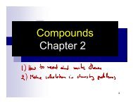
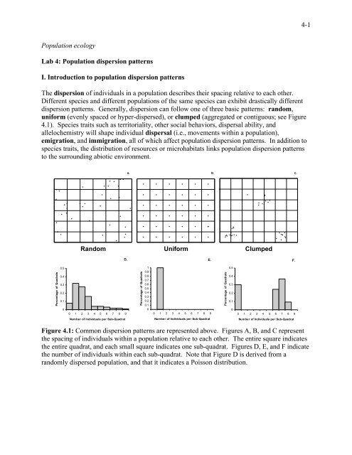
4-1Population ecologyLab 4: Population dispersion patternsI. Introduction to population dispersion patternsThe dispersion of individuals in a population describes their spacing relative to each other.Different species and different populations of the same species can exhibit drastically differentdispersion patterns. Generally, dispersion can follow one of three basic patterns: random,uniform (evenly spaced or hyper-dispersed), or clumped (aggregated or contiguous; see Figure4.1). Species traits such as territoriality, other social behaviors, dispersal ability, andallelochemistry will shape individual dispersal (i.e., movements within a population),emigration, and immigration, all of which affect population dispersion patterns. In addition tospecies traits, the distribution of resources or microhabitats links population dispersion patternsto the surrounding abiotic environment.A. B. C.Random Uniform ClumpedD.E.F.Percentage of Quadrats0.50.40.30.20.100 1 2 3 4 5 6 7 8 9Percentage of Quadrats10.90.80.70.60.50.40.30.20.100 1 2 3 4 5 6 7 8 9Percentage of Quadrats0.50.40.30.20.100 1 2 3 4 5 6 7 8 9Number of Individuals per Sub-QuadratNumber of Individuals per Sub-QuadratNumber of Individuals per Sub-QuadratFigure 4.1: Common dispersion patterns are represented above. Figures A, B, and C representthe spacing of individuals within a population relative to each other. The entire square indicatesthe entire quadrat, and each small square indicates one sub-quadrat. Figures D, E, and F indicatethe number of individuals within each sub-quadrat. Note that Figure D is derived from arandomly dispersed population, and that it indicates a Poisson distribution.

4-2II. Measuring population dispersionPopulation dispersion is commonly quantified by population ecologists. With mobile organisms,this requires intensive sampling; therefore, we will measure the dispersion patterns of less mobilespecies. Analyses of population dispersion patterns usually follow a standard method in whichobserved patterns are compared to predicted, random dispersion patterns modeled on the Poissondistribution. Deviations from the predicted, random pattern suggest that the population understudy exhibits either a uniform or clumped dispersion pattern. In today’s lab exercise, we willutilize two different techniques to characterize the dispersion pattern of our focal species: (1) aquadrat-based method and (2) a point-to-plant method.Quadrat MethodThe quadrat method involves counting the frequency of occurrences of the species of interest ineach of the 100 individual 10 X 10 cm sub-quadrats that compose the 1 m 2 quadrat. If theindividuals within the population are randomly dispersed, there will be a random number ofindividuals in each quadrat, centered about the mean (see Figure 4.1 A & D). If the individualsin the population are uniformly dispersed, there will be the same number of individuals in eachsub-quadrat (see Figure 4.1 B & E). If the individuals in the population are clumped indispersion, there will be a few quadrats with many individuals, and many quadrats with noindividuals (see Figure 4.1 C & F).To analyze the data from the quadrat method we will use a chi-square test of hypothesis. Thechi-square test compares a given distribution to the Poisson distribution. We will use anequation to generate a Poisson distribution with the characteristics that we would expect from arandomly dispersed plant species that has a mean number of plants per sub-quadrat equal to oursample population. This equation is called the ‘Poisson expression’ by Cox (2001), and it lookslike this:…where e = the base of the natural log = 2.7182818, µ = mean, and x = the frequency category.In Excel, the formula would look like this:=(µ^x)/((EXP(µ))*(FACT(x)))For example, we sample 40 sub-quadrats/cells. Nine cells have 0 individuals, 22 have 1individual, 6 have 2, 2 have 3, 1 has 4 and none of the quadrats/cells have 5 or more individuals(Table 1). Given these values, we can calculate the Poisson probability P(x i ) for each category.

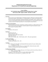
4-3Table 1: Example data -- there are 40 total sub-quadrats, 44 total individuals, and a mean of 1.1individuals per sub-quadrat.Number ofIndividuals perSub-Quadrat(x i )Number ofSub-Quadrats(f i )f i x i0 9 9 * 0 = 91 22 1* 22 = 222 6 2 * 6 = 123 2 3 * 2 = 64 1 4 * 1 = 4≥5 0 5 * 0 = 0Σ 40 441.1To calculate the mean value for data in this format use the following equation:…where f is the number of sub-quadrats and x is the number of individuals per sub-quadrat foreach row in Table 1. We can use the Poisson probabilities to generate expected probabilitieswith which we can calculate expected values for each row in Table 1.We can then use these expected probabilities to calculate expected values using the equationbelow (essentially, multiply each probability above by the total number of quadrats, in this case,40.):Use these expected values to compare with our observed values using a chi-square test. The teststatistic for the chi-square test is χ 2 :In this example, the expected values for quadrats with three or more individuals are combined forthe χ 2 analysis because those quadrats have small sample sizes (2 quadrats with 3 individuals, 1quadrat with 4 individuals, and no quadrats with 5 individuals). If the expected frequency forany category is less than 1, you must add them together, using summed fi values to calculate χ 2(see Table 2). You will also need to calculate the degrees of freedom to locate the χ 2 statistic ona table:df = k-2

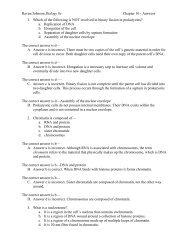
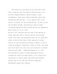
4-4…where k is the number of categories remaining after you perform any necessary adding (2 inour example, Table 2). The χ 2 statistic for our example is 5.841 (Table 2). You can look this upon the χ 2 table, or use the following Excel formula to get a precise p-value:=CHIDIST(χ 2 ,df)…where χ 2 is the test statistic you calculated and df are the degrees of freedom.Table 2. Example of a Poisson Table -- Asterisk (*) denotes that the categories for 3, 4, and 5individuals per quadrat were combined into one class in order to better meet assumptions of theχ 2 test.Number ofObservedindividualsFrequencyper quadrat(O)(x i )P(x)ExpectedFrequencyE (O-E) 2 /E0 9 0.332871 13.315 1.3981 22 0.366158 14.646 3.6922 6 0.201387 8.055 0.5243 2 0.0738424 1 0.020307 3.945* 0.226*5 0 0.004467Σ 40 1 5.841By plotting the observed and expected values from Table 2, we can see that our data conformclosely to the Poisson distribution (Graph 1).Graph 1. Graph of example data.

4-5Point-to-plant MethodThe point-to-plant distance method utilizes a ratio to detect deviation from a random dispersionpattern. We use this method to sample dispersion for organisms that cannot easily be sampledusing a 1 m 2 quadrat (like trees or species that occur much more spaced out). To collect theappropriate data, you will haphazardly select a point of origin (by throwing an object of somesort), and then measure the distance from that point to the nearest two individuals of the speciesof interest. Each team will measure 10 haphazardly selected points. These data will be used tocalculate the sample coefficient of aggregation (A):…where n = the number of sample points, and d = the distance from the selected location andtree 1 or 2. The closest tree should be recorded as d 1 .This coefficient of aggregation will always be between 0 and 1, and the expected value of A for arandomly dispersed population is 0.5. The z-equation is used to determine if A is significantlydifferent from 0.5:…where n = the number of sample points, 0.2887 = the standard deviation of A values for arandomly dispersed population. The calculated z is looked up on the z table to find a p-value forthe null hypothesis that A is not significantly different from 0.5. You can use excel to look up aprecise p-value from the z-table (z is your calculated z-value):=1-NORMSDIST(z)If A is significantly less than 0.5, the dispersion is uniform, and if A is significantly greater than0.5, the dispersion is aggregated. Note that this is very similar to the equation for a t-test fromthe first lab. The z-equation is simply a special version of the t-equation, except that the degreesof freedom are irrelevant because the number of sample points (n) must always be greater than30, and the population variance must be known.III. ObjectiveThe field portion of today’s lab will involve collecting data on the dispersion pattern ofpopulations of a small, herbaceous plant and a large tree species chosen by your TA. Theobjective of Lab 4 is determine if the dispersion patterns of the populations you investigate arerandom, uniform, or clumped.

4-6IV. InstructionsBefore setting out to sample your focal species, complete the following pre-field instructions:1) Generate several testable hypotheses as a class that you can test with today’s exercise.2) Discuss how to record the 2 different kinds of dispersion data. Set up field datasheets for your sampling procedures.3) Divide into groups and work as teams in the field. Work should be divided up so thatall team members get to experience each aspect of the exercise.4) Be sure that you have all the field sampling equipment that you will need.5) All field teams should participate in sampling all habitats. Your TA will pool datafrom all teams to generate larger datasets for each population that you investigated.Use these complete datasets for your analysis.Field instructions:Sampling for the quadrat method will involve 1 m x 1 m quadrats that are divided into 100 subquadratseach 10 cm x 10 cm. Randomly locate your group’s quadrat within the populationidentified by your TA and determine how many individuals of the species indicated by your TAyou find in your quadrat. Record data for each species by counting the number of individuals ofthe given species in all of your 100 sub-quadrats. Keep track of which grid you are counting(e.g., by using numbers to label columns and letters to label rows, then identifying each grid witha number-letter designation).To perform the point-to-plant distance method, locate the required number of random points inthe population of interest. Measure the distance from each random point to the two nearest treesof the focal species. Once you are finished, you will have two distances (in meters) for eachrandom point: the distance from the point to the nearest tree and the distance from the point tothe next nearest tree. You will use these data to calculate the coefficient of aggregation (A) foryour focal population in order carry out the z-test to determine the dispersion pattern of thepopulation.

4-7Literature CitedCox, G. W. 2001. General Ecology Laboratory Manual, 8th edition. McGraw-Hill, New York.Further ReadingCornell, H. V. 1982. The notion of minimum distance or why rare species are clumped.Oecologia 52(2):278-280.Zavala-Hurtado, J. A., P. L. Valverde, M. C. Herrera-Fuentes, A. Diaz-Solis. 2000.Influence of leaf-cutting ants (Atta mexicana) on performance and dispersion patterns ofperennial desert shrubs in an inter-tropical region of Central Mexico. Journal of AridEnvironments 46(1):93-102.