DRAFT: US-JAPAN PBEE PAPER BY CORDOVA ... - PEER

DEVELOPMENT OF A TWO-PARAMETER SEISMIC INTENSITYMEASURE AND PROBABILISTIC ASSESSMENT PROCEDUREPaul P. Cordova 1 , Gregory G. Deierlein 2 , Sameh S.F. Mehanny 3 , and C.A. Cornell 4ABSTRACTA method to evaluate the seismic collapse performance of frame structures is presented,considering uncertainties in both the ground motion hazard and inelastic structural response toextreme input ground motions. The procedure includes a new seismic-intensity scaling indexthat accounts for period softening and thereby reduces the large record-to-record variabilitytypically observed in inelastic time-history analyses. Equations are developed to combine resultsfrom inelastic time history analyses and a site-specific hazard curve to calculate the mean annualprobability of a structure exceeding its collapse limit state.1. INTRODUCTIONResearch on performance-based earthquake engineering poses many challenges, among thembeing the need for a consistent methodology to predict structural collapse as a function of theearthquake ground motion intensity. Components to an assessment methodology for collapseshould include (1) definition of the seismic hazard, (2) simulation of structural response to inputground motions, including stiffness and strength degradation, and (3) statistical interpretation ofresults. The methodology must rigorously account for variability in performance predictionarising due to uncertainties in the inherent seismic hazard and the nonlinear simulation ofstructural response.A large source of variability in seismic performance assessment arises from simplifications indefining earthquake intensity relative to the true damaging effects of ground motions onstructures. Current codes in the United States, such as the International Building Code (ICC2000), define earthquake hazard in terms of spectral response coefficients, typically spectralacceleration measured at the first mode period of vibration, S a (T 1 ). First mode spectralacceleration is the basis of equivalent lateral force design procedures, and it is often used as thedefault earthquake intensity scaling parameter for time-history analyses. While first mode1 Research Assistant, John A. Blume Earthquake Engineering Center, Stanford Univ., Stanford, CA 94305-40202 Prof., Dept. of Civil & Env.l Engrg., Stanford Univ., Stanford, CA 94305-4020, email: ggd@stanford.edu3 Simpson Gumpertz and Heger, Inc., San Francisco, CA., email: SSFMehanny@sgh.com4 Prof., Dept. of Civil & Env.l Engrg., Stanford Univ., Stanford, CA 94305-4020, email: cornell@ce.stanford.edu1

spectral acceleration is an accurate index for structures that respond elastically, this singleparameter does not reflect many of the aspects of earthquake ground motions that affect inelasticstiffness and strength degradation. An objective of this paper is to examine a new two-parameterhazard intensity index that can improve the accuracy of structural performance predictions basedon inelastic time history analyses. A related objective is the development of reliability-basedequations for interpreting the performance limit state to compare the effect of using a singleversus two-parameter intensity measure.The scope and approach of this paper is as follows. First, the general concepts of earthquakeground motion intensity measures are introduced, including an overview of traditional measuresand the development of attenuation functions for the new proposed index. Second, a series ofcase study buildings are introduced and analyzed to determine their collapse limit state usingincremented inelastic time-history analyses coupled with a post-earthquake stability analysis.Results of the case study analyses are used to calibrate the new earthquake intensity measure.Next, a probability-based assessment procedure is developed to describe the collapseperformance in terms of mean annual probability of exceedance and an equivalent load andresistance format. Finally, the probabilistic assessment procedure is demonstrated through anapplication to one of the case study buildings.2. HAZARD INTENSITY MEASURESTraditionally, building codes have quantified earthquake intensity as a function of either peakground motions (acceleration or velocity) or linear response spectrum quantities (acceleration,velocity, or displacement). As implied by their name, linear response spectrum quantities do agood job at characterizing earthquake effects in structures that respond elastically, but they donot necessarily capture inelastic behavior. More elaborate indices, which seek to improvecharacterization of earthquake ground motions, have been the subject of continuing studies. Forexample, Housner (1975) proposed combining spectral acceleration together with strong motionduration. More recently, Luco (2001) has proposed extending linear spectral quantities into thenonlinear realm through the use of inelastic spectral response demands. While they are generallymore accurate, one drawback of the nonlinear spectral values is that they imply a couplingbetween the earthquake hazard definition and the inelastic structural properties. This complicates2

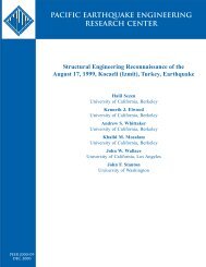
development of seismic hazard maps for general use. Another topic of recent research concernsnear fault directivity effects and whether these warrant specialized treatment in earthquakehazard characterization (e.g., Alavi & Krawinkler 2000). These are just a few examples ofresearch to investigate the damaging features of earthquake ground motions and developimproved hazard intensity measures to represent these effects.Common to most studies of improved intensity measures is the goal to characterize groundmotion hazards in a statistically meaningful way for predicting structural performance. Thisimplies that the best intensity measures are those that result in the least record-to-recordvariability, measured with respect to a common intensity index, when evaluating structuralperformance to multiple earthquake records. Of course, even with the best ground motioncharacterization, uncertainties will persist in characterizing the geologic earthquake hazard andin simulating inelastic structural performance.αImproved Hazard Intensity Measure - S a (T 1 )R SaThe International Building Code (ICC 2000) and most other earthquake engineering designstandards in the United States define hazard intensity as the spectral acceleration of the groundmotion, typically calculated at the fundamental (first mode) period of the structure. A knownshortcoming of this measure is that it does not account for inelastic lengthening of the period asthe structure softens under stiffness degradation. As illustrated in the response spectra plots ofFig. 1, two ground motionscharacterized on the basis of their firstmodespectral response may result insignificantly different inelasticresponse, depending on the slope ofthe spectra at lengthened periods. Forexample, when normalized withrespect to S a (T 1 ), record #2 willinevitably produce larger inelasticdeformations than record #1. Thistrend is not accounted for in the singlespectral quantity, S a (T 1 ).3S aRecord #1S a (T 1 )Record #2As damage occursT 1T FS a (T F )T, PeriodFigure 1 – Effects of structural softening.

A simple extension to current practice that can help capture the period shift effect is to introducea second intensity parameter that reflects spectral shape. The proposed parameter to do this is aratio of spectral accelerations at two periods,Sa( Tf)RS a= (1)S ( )aT 1where T 1 is the first mode period and T f is a longer period that represents the inelastic (damaged)structure. This ratio can then be combined with the first mode spectral acceleration, S a (T 1 ), togive the following new two-parameter hazard intensity measureαa( T 1R SaS * = S )(2)where α and the ratio T f /T 1 are determined by calibration to optimize the intensity index byminimizing the variability in computed results.Attenuation Functions for Two-Parameter IndexGiven the prevalence of linear spectral acceleration in codes and practice, most hazardassessment techniques and data are geared toward this predicting this quantity. For example,national hazard maps available from USGS define earthquake hazard in terms of spectralacceleration at two periods (roughly T = 0.2 second and 1 second) representative of short andlong period structures. In devising new intensity measures, it is convenient if they can bederived by manipulating existing models and hazard data.Since the proposed intensity measure, S * , is simply a function of the spectral acceleration at twodifferent periods (T 1 and T f ), it is relatively straightforward to modify existing attenuationfunction to accommodate this index. Equations 3 and 4 show the transformation of a singleparameter attenuation function, E[ln S a (T x )], to the modified function, E[ln S * ], where E[ln …] isread as the “expected value of the natural log of the given parameter” and other variables are asdefined previously:*ln S = (1 −α )ln Sa( T1) + α ln Sa( Tf)(3)*[ S ] (1 −α ) E[ ln S ( T )] + αE[ ln S ( T )]E ln =a 1a f(4)In addition to the expected value of S*, the standard deviation, σln S*, must also be defined. Thisin turn requires the correlation between spectral accelerations at the two periods, S aT ) and( 14

S a( T f) . Inoue (1990) provides the following empirical correlation coefficient, ρln Sa1ln Sa f, thatfills this need:ln Sa1ln Sa f( T ) − ln( 1/ T )ρ = 1−0.33ln 1/1f(5)Given this correlation expression, the standard deviation of S* can be defined as follows:σ2 22 2( 1 − α ) σln Sa+ α σln Sa+ 2ρ( )1 f ln Sa1ln Sa1 − α ασfln Saσln Sa f= (6)2ln S*1Most spectral attenuation relationships define empirical coefficients as a function of frequency orperiod that can be manipulated to calculate S* according to Eq. 4. For example, Abrahamson &Silva (1997) define an attenuation function as follows:n[ S ] a + a (m-m ) + a ( 8.5-m)+ [ a a (m-m )] ln(R)E ln =1 4 1 123+13 1(7)awhere the a-coefficients are tabulated by Abrahamsom & Silva, m is the earthquake magnitude,m 1 is a given base magnitude, and R is the distance from the epicenter to the site. SubstitutingEq. 7 into Eq. 4, one obtains the following relationship for modified coefficients that can beapplied in the otherwise standard attenuation relationship to obtain S*:a*x= a a(8)( 1−α )xT1+ αxT 2These new relationships can then be applied in a standard probabilistic site hazard analysis wherethe required performance is evaluated on the basis of this new intensity, S*.3. BUILDING TESTBEDSIn related research (Mehanny et al., 2000, 2001) several moment frame structures have beendeveloped and analyzed to exercise seismic assessment and design provisions for compositeconstruction. These frames are utilized here to provide the basis for calibrating the new intensitymeasure parameters, α and T f /T 1 , and illustrate their application in a probabilistic performanceassessment. The case study structures consist of three six-story frames and one twelve-storyframe, all of which are designed according to provisions of the International Building Code (ICC2000) and AISC Seismic Provisions (1997) for a site in a high seismic region of California. Dueto space limitations the frames are only briefly introduced here. For further details the reader isreferred to Mehanny et al. (2000, 2001).5

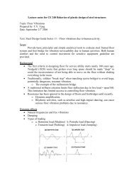
Three of the case study structures are composite moment frames composed of reinforcedconcrete columns and steel beams (referred to as RCS systems), and the forth is a steel spaceframe. An elevation of one of the frames, a six-story RCS perimeter frame, is shown in Fig. 2.Beam sizes in the frames were generally governed by drift requirements while the reinforcedcolumns were governed by the strong column weak beam criterion. As summarized in Table 1,vibration periods for the frames range from T 1 = 1.3 to 2.1 seconds (note – other data reported inTable 1 is discussed later).Inelastic static and dynamic (time history) analyses are conducted using an analysis programdeveloped by El-Tawil et al. (1996) that takes into account second-order geometric behavior andspread-of-plasticity effects in the beam-columns and connections. Inelastic componentproperties are based on the expected (as compared to nominal) material strengths, where theexpected strengths are taken as 1.15 times the nominal strengths. Static pushover and inelastictime history analyses are run simultaneously with gravity loads equal to 100% dead load and25% live load. Summarized in Table 1 are static lateral overstrengths of the frames, defined asΩ o = V u /V d where V u is the ultimate base shear and V d is the IBC design base shear. Theoverstrengths range from roughly Ω o = 2.6 for the six-story RCS perimeter frame up to Ω o = 6.1for the six-story steel space frame. The overstrengths are relatively large compared to the typicalexpected values of Ω o = 2 to 3, due to the following sources of overstrength: (1) expected versusminimum specified material strengths, (2) minimum stiffness (drift) criteria, (3) structuralredundancy, (4) strong column criterion, and (5) discrete member sizing.Frame IDFirstModePeriod,T 1 (sec)V u /V d ,ΩTable 1 – Testbed frame dataσ ln(IDR|Sa)6S_RCS_S 1.3sec 3.9 0.426S_S_S 1.3sec 6.1 0.2712S_RCS_S 2.1sec 4.4 0.246S_RCS_P 1.5sec 2.6 0.30IDA Dispersion Data for Alternative Intensity MeasuresGeneral RecordsNear Fault Recordsσ ln(IDR|SaRsa)(Optimized)0.28(1.9,0.65)0.20(1.2,2.4)0.19(1.6,0.6)0.23(1.65,0.45)σ lnIDR|SaRsa(2.0,0.5)σ ln(IDR|Sa)0.29 0.450.23 0.300.22 0.26σ ln(IDR|SaRsa)(Optimized)0.22(1.8,0.9)0.18(1.6,0.8)0.21(2.4,0.4)σ ln(IDR|SaRsa)(2.0,0.5)0.270.190.220.24 - - -6

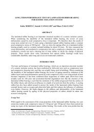
6 @ 4m = 24mW530x92W610x101W610x101600 x700mm650 x750mmS a (g)432RCS PerimeterT1 = 1.50 secIV79-A6LP89-LGLP89-LXEZ92-EZNR94-NHNR94-RSNR94-SYKB95-JM2%in50yr12 @ 6.4m 9.6m35.2m2 @ 6.4mFigure 2 –Elevation of RCSperimeter frame.00.0 0.5 1.0 1.5 2.0 2.5 3.0 3.5 4.0Period (sec)Figure 3 – Near FaultResponse Spectrum4. COLLAPSE ANALYSIS TECHNIQUESIncremented Dynamic AnalysisSeismic performance is assessed through nonlinear time history analyses using two sets ofground motions – one comprised of eight general records and another of eight near-fault recordswith forward directivity. Response spectra for the near-fault records are superimposed on the2% in 50-year design hazard spectrum used to design the case study buildings in Fig. 3.Acceleration components of the records are scaled, where the resulting ground motion intensityis reported in terms of either spectral acceleration, T ) , or the proposed new index,S a( 1aR SaαS .Shome and Cornell (1997) have demonstrated that such scaling of records will not bias theresults and is an appropriate technique for multi-level hazard analysis. More details on theground record properties and scaling issues for the records are summarized by Mehanny (2000).Results of the time history analyses are summarized by plotting the scaled intensity measureversus maximum Interstory Drift Ratio (IDR), creating what are referred to herein asIncremented Dynamic Analysis (IDA) curves. Shown in Fig. 4 are examples of the IDA curvesfor the RCS perimeter frame building subjected to the general records, where each data pointcorresponds to the peak IDR resulting from a single time history analysis. The collection of datapoints for a single ground record scaled to multiple hazard levels forms the IDA curve. Resultsare plotted in terms of the S aT ) intensity in Fig. 4a and( 1aR SaαS in Fig. 4b.7

S a (T 1 ,5%)2.52.01.51.0CM92-RIOLA92-YERLP89-HCALP89-HSPLP89-WAHOMiyagiMendocinoValparaisoS a R Saα1.51.00.5α = 0.45T F = 1.65T 10.50.00.00.00 0.02 0.04 0.06 0.08 0.10 0.12 0.00 0.02 0.04 0.06 0.08 0.10 0.12IDR MAXIDR MAX(a)(b)αFigure 4 – IDA plots for 6S_RCS_P Frame: (a) IDR vs. S a (T 1 ) (b) IDR vs. S a R saComparing the graphs in Fig. 4, it is obvious that the two-parameter intensity measure (Fig. 4b)results in significantly less record-to-record variability than S aT ) (Fig. 4a). The variability canbe quantified in terms of dispersion of the drift response conditioned on the ground motionintensity measure. Dispersion is calculated according to the following equation as the meansquared deviation of the drift data from an average response curve obtained by linear regressionin log-log space between drift and the seismic intensity (of the form, ln IDR MAX = A + B ln IM):( 1where⎡2(ln1 ,− ln ˆ ) ⎤=ln⎢∑ nIDR IDRi=MAX iMAXσIDR MAX1⎥(9)intensity measure⎢n −⎣⎥⎦IDRMAX , iis the ith response calculated for a given intensity, DRMAX12I ˆis the value from theregression curve, and n is the total number of observations (n=8 in this case).Comparing Figs. 4a and 4b, the dispersion σ ln(IDR,Sa) = 0.45 for the S a (T 1 ) index is roughly twicethat of σ ln(IDR,SaR) = 0.22 forS aR Saα. This result is based on using the optimized coefficients ofαα=0.45 and T f /T 1 =1.65 for the S index, determined by varying these factors so as toaR Saminimize the dispersion. Note that these optimal values are specific to the RCS six-storyperimeter frame under the set of eight ground motions. Reduction in the dispersion in this wayhelps reduce the number of records necessary to simulate time history response within aspecified confidence interval.8

While the two-parameter index reduces the overall dispersion, this reduction is most apparent atlarger drifts, where the structure behaves nonlinearly. In fact, comparing Figs. 4a and 4b, in theelastic range (at lower drifts), the two-parameter S index results in more variability thanSa(T 1 ). This follows from the fact that Sa(T 1 ) provides a nearly exact correlation with drift forthe linear case, whereas the period shift captured in S works best when the structurebehaves nonlinearly. This suggests that an improved index would be one where the α and T fparameters are devised to vary with the degree of inelastic action, similar in some ways to howthe period is shifted using the capacity spectrum method for calculating the target displacementfor nonlinear static pushover analyses.aR SaαaR SaαWhile the IDA’s provides useful information on the structural response, it is apparent from thecurves in Fig. 4 that the IDA’s do not reveal a definitive stability limit state. Some curves, suchas the one for the LP89-HCA record, asymptotically approach a bounding strength (in terms ofthe intensity measure), but others do not. For example, the CM92-RIO and Valparaiso plotsmaintain positive slopes at very large earthquake intensities and drifts. This reflects inherentlimitations of the inelastic time-history analysis to fully capture the strength and stiffnessdegradation at large inelastic deformations.Frame Stability Limit State DeterminationTo evaluate global instability, the authors have employed a procedure that integrates localdamage indices, computed during the time-history analysis, through a supplementary stabilityanalysis of the damaged structure. The basic procedure, described in detail by Mehanny andDeierlein (2001), entails a post-earthquake second-order inelastic stability analysis to assess theloss of gravity load capacity due to damage incurred during the earthquake. This procedure,which leads to the plot of an intensity measure versus gravity stability index λ u shown in Fig. 5,entails three basic steps. (1) Perform a nonlinear time-history analysis and calculate thecumulative damage indices. This provides the basis to quantify the localized (distributed)damage caused by a given earthquake ground motion. The damage indices are empiricalequations that track the structural damage as a function of cumulative plastic deformations. (2)Modify the analysis model based on the damage incurred during the time-history analysis. This9

involves reducing element stiffness and strengths as a function of the cumulative damage indicesand incorporating the residual (permanent) building drift into the structural topology. (3)Reanalyze the modified structural model through a second-order inelastic static analysis undergravity loads up its inelastic stability limit. The resulting stability index, λ u in Fig. 5, is definedas the ratio of the vertical load capacity to the applied gravity loads, where the gravity loads areassumed as full dead load plus 25% of the live load.The stability index, λ u , provides a global failure criterion that integrates the effect of localdamage sustained under each earthquake record and intensity. Figure 5 shows the evolution ofthe stability index for the six-story RCS space frame, where there is a one-to-one correspondencebetween stability points in Fig. 5 and the maximum interstory drifts in Fig. 4. The initial valueof λ uo = 5.5 (on the horizontal axis in Fig. 5) is the index for the undamaged structure, implyingthat the undamaged frame has sufficient lateral strength/stiffness to maintain stability under 5.5times the gravity load. This large value reflects the fact that the structure has significant gravityloadoverstrength as a result of the high seismic loads. The point where the curves cross λ u =1.0is point at which the structure can no longer sustain stability under its self-weight due toextensive seismic damage. The stability index at this point is defined as λ f and the associatedmedian value of the seismic hazard value isµˆλ f. This level is defined as the ‘capacity’ – orcollapse limit state – of the structure. Between these limits, λ uo and λ f , a third limit point isidentified at λ u = 0.95λ uo , corresponding to the point at which the lateral stability begins to2.52.01.5α = 0.45T F = 1.65T 1S a (T 1 ,5%)1.51.0S a R S a α1.00.50.5λ u = 1.0λ u = 0.95λ uo0.00 2 4 6 8 10 12 140.00 2 4 6 8 10 12 14IDR MAXIDR MAX(a)(b)Figure 5 – Stability curves versus IM, (a) IM = S a , (b) IM = S a R saα10

significantly degrade. This point, referred to as λ OD (Onset of Damage) defines where there is asharp transition in the S aT ) or( 1aR SaαS versus λ u stability curve, representing the intensity levelbeyond which the stability index degrades rapidly.Similar to the IDA plots (Fig. 4), the S aT ) index shows much larger record-to-recordα( 1variability in the λ u response than the S index. The standard deviations of S aT ) at λ ODaR Saand λ f are equal to 0.40 and 0.49, respectively, compared to 0.26 and 0.15 using( 1SaR Sareduced variability leads to a better approximation of the expected collapse performance.α. This5. DETERMINATION OF GENERAL α AND T fThe examples described above show how the proposed intensity measure,SaR Saα, cansignificantly reduce the record-to-record variability in calculating the seismic performance.What remains to determine is optimum values of α and the period multiplier, C=T f /T 1 , whichminimize dispersion for a broad class of building frames. To accomplish this, we will utilizeanalysis results of the four case study structures introduced previously.To determine the optimal calibration for α and C, IDA and λ u stability analyses are run for eachof the four structures under the sixteen ground motions (eight general and eight near fault).Next, theSa R Saαresponse data is plotted for various combinations of α and C, the averageresponse curve is fit to the data, and the dispersion is calculated. This results in many α and Cpairs for each structure, each with its own dispersion, σ lnIDR . The optimal α and C pair for eachstructure is one that yields the least dispersion. The graphs in Fig. 6 show the resultingrelationships between α, C, and the resulting dispersion for each structure and bin of groundmotions. The optimum alpha-coefficient is plotted versus the corresponding C in Fig. 6a, and theassociated dispersions for the corresponding pairs of α and C are plotted in Fig. 6b.Determination of one general pair of α and C obviously compromises the preciseness that can beachieved with multiple pairs tailored for each structure and each ground record. Nevertheless, a11

Alpha-Coefficient2.06_RCS_S, gen1.8 mean = 0.496_RCS_S, nf1.6 median = 0.45 α6_S_S, gen1.4 σ = 0.1256_S_S, nf12_RCS_S, gen1.212_RCS_S, nf1.06_RCS_P, genCase Study, Fig. 4b0.80.60.40.2(1.65,0.45)0.01.2 1.4 1.6 1.8 2.0 2.2 2.4 2.6 2.8 3.0Multiplier, C(a)Figure 6 – Optimization of S a R α Sa ,(a) Range of optimum α-C pairs and (b) Dispersion on α-C pairs.common calibration is desired to make the procedure convenient for generalized use. Referringto Fig. 6b, on average the dispersion turns out to be relatively constant over a large range of Cand α pairs. Further, from Fig. 6a we see that the optimal α (given C) is relatively stable for 2

already low when scaled by spectral acceleration alone. Comparing results for the average twoparameterindex (Eq. 10) with Sa(T 1 ), the two-parameter index reduces the range of dispersionfrom 0.24-0.45 for Sa(T 1 ) to 0.19-0.29 for SaR Sa 0.5 .S a R Saα1.00.5α = 0.5T F = 2.0T 1CM92-RIOLA92-YERLP89-HCALP89-HSPLP89-WAHOMiyagiMendocinoValparaisoαS a R Sa1.00.5α = 0.5T F = 2.0T 10.00.00 0.02 0.04 0.06 0.08 0.10 0.12IDR MAX0 2 4 6 8 10 12 14λ u(a)(b)0.5Figure 7 – Updated Behavior Curves with IM = S a R Sa(a) IDA and (b) stability curves0.06. PROBABILITY ASSESSMENT OF COLLAPSE PREVENTIONUsing the inelastic time-history and stability analysis method described above, the “collapseprevention” performance for a given set of ground motion records is defined by the stabilitylimit,µˆλ f, defined in terms of the seismic hazard intensity – either Sa(T 1 ) or SaR 0.5 Sa . The nextstep in the performance assessment is to compare the stability limit to the seismic hazard,considering the uncertainty in both the calculated response indices and the site hazard curve.Mean Annual Probability of ExceedanceDefining failure (collapse) by the likelihood of the ground motion intensity exceeding thestability limitP fµˆλ fthe mean annual probability of collapse can be described by the following:[ ≥ µˆ ]= P IM(11)λfWhere P f is the mean annual probability of failure and IM is the seismic hazard demandexpressed using an intensity measure consistent with that used to define the stability limit,µˆλ f.In this case, the two alternative intensity measures considered are S aT ) or( 1SaR Sa0.5. The13

seismic demands are expressed in terms of a probabilistic hazard curve (the annual probability ofexceeding a specified intensity measure), determined either explicitly by a probabilistic seismichazard analysis or using published hazard maps.Equation 11 can be further expanded into the following form using the total probability theorem:∞∫0Pf = HIM( u)fλ( u)du(12)fWhere u is the intensity measure, H IM (u) is the hazard curve, andλ(u)is the probabilitydensity of the structural stability limit. To permit closed-form solution of the probabilityintegral, the hazard function is assumed to take the following form:H−kIM( u)= kou(13)where k o and k are coefficients that fit Eq. 13 to the hazard data. Further, (u)is assumed as afffλ flognormal distribution with the medianµˆλ fand the dispersion δ λf (or σ ln(λf) ). Given theseassumptions, the integral solution to Eq. 12 is as follows:Pf122 2δ λ f= H ( ˆ ) e(14)IMµ λfkwhere H IM ( µˆ ) is the mean annual probability from the hazard curve evaluated at the mediancapacityλ fµˆλ f, and the other terms are as defined previously.LRFD-like Format of Collapse ProbabilityAn alternative way to envision the mean annual collapse probability is by rearranging Eq. 14 soas to compare the hazard demand to the structural capacity in a format similar to that used forLoad and Resistance Factor Design (LRFD) provisions. Setting the failure probability in Eq. 14to a maximum acceptance probability criteria, P f < P acceptance , Eq. 13 and 14 can be combined togive the design requirement:−kk δ2 λ fˆo λe

whereIM is the hazard intensity measure with the annual probability, Pacceptanc, of beingetanP accepceexceeded (i.e. P = H IM ) ). The term,acceptanceIM(P acceptanc ee122kδλ f, which reflects the variability ofthe median stability limitµˆλ f, can be moved to the left side of Eq. 16, resulting in the following:e− 1 2kδ2 λfˆ µλf≥ IMPacceptanceorφ ˆ µλf≥“seismic demand” (17)where φ = e2− 1 kδ2 λ f. This equation is similar to LRFD equations that are prevalent in codeprovisions where the “design strength” on the left side (the nominal strength reduced by a phifactor) is compared to the load effect or “seismic demand”. In this case there is no load factor onthe seismic demand since the recurrence interval of the demand is implicit in its definition.An important but perhaps misleading coincidence in Eq. 17 is that the probability associated withthe demand term (on the right side) turns out to be equal to the desired limit on the probability ofexceeding the median stability intensity,µˆλ f. This is different than saying that one is designingfor a given hazard with a specified probability of exceedance. From Eq. 15, the underlyingprobability statement implied in Eq. 17 is related to the likelihood of exceeding the stabilitycriterion,µˆλ ftaking into account both variability in the ground motion hazard and the record-torecordvariability in the stability index.Essentially, Eq. 17 enables one to establish whether a structure meets the collapse performanceobjective with a mean annual probability of exceedance, P acceptance . There are two basic inputrequirements for the procedure: (1) the “seismic demand” for the desired probability ofexceedance, IM P,acceptance , determined using either hazard maps or a probabilistic seismic hazardanalysis; and (2) the median stability limit,dispersion δλfor a representative set of ground motions.fµˆλ, of the structure and the correspondingf7. APPLICATION OF PROBABILISTIC COLLAPSE ASSESSMENTThis example will go through a collapse performance assessment for the 6-story RCS perimeterframe. The hazard analysis is based on a site at Yerba Buena Island (in San Francisco Bay)15

where the San Andreas and Hayward faults govern the seismic hazard. The seismic hazard ischaracterized two ways: (1) through an explicit probabilistic seismic hazard analysis of the siteand (2) using spectral acceleration hazard maps from building code provisions.Annual Hazard CurvesProbabilistic Seismic Hazard Analysis (PSHA): Using the Abrahamson and Silva attenuationrelationship presented in Eqs. 7 and 8, annual hazard curves for spectral acceleration, S aT ) ,and the proposed intensity measure,SaR Sa0.5( 1, can be developed through a standard probabilisticseismic hazard analysis for the Yerba-Buena Site site. Details of the hazard analysis are beyondthe scope of this paper, but basically, this analysis provides a probabilistic assessment ofearthquake magnitude and distance (M-R) pairs for the site, given its proximity to nearby faults.Code Based Technique: An alternative (simplified) technique to obtain the hazard curve is toinfer it from mapped spectral and site coefficients such as those provided by the seismic designprovisions of the International Building Code (ICC 2000). The first step is to calculate thespectral acceleration for the site using the following equation:F SSv 1a= (18)T1where F v is a tabulated site coefficient, given as a function of the site (soil) class and the spectralcoefficients, and S 1 is the spectral hazard coefficient obtained from seismic hazard maps with aan average probability of occurrence of 2% in 50-years. Implied by Eq. 18 is a 1/T spectralcurve in the long period range. Using Eq. 18, one can directly obtain the 2% in 50 year (P o =0.0004) spectral acceleration at the first mode period T 1 , i.e., S a (T 1 ). One can also approximatethe two-parameter index0.5SaR Sa, by assuming that RS a2 = Sa( T1 ) / Sa(2T1) = 2T1/ T1= . Twoapproximations inherent in this assumption are that there is full correlation between the hazardvalues of S a (T 1 ) and S a (2T 1 ) and the 1/T design spectrum accurately represents the hazardspectrum. Once the 2% in 50 year spectral values are known, the full hazard curve is constructedassuming k = 4, and then back-calculating the k o parameter.Hazard Curve Comparison: Hazard curves for T 1 = 1.5 seconds (the natural period for the sixstoryRCS perimeter frame) are shown in Fig. 8, and the corresponding hazard curve parameters16

1e-1IBC CodeY-B PSHA1e-1IBC CodeY-B PSHAMean Annual Prob. [S a >x]1e-21e-31e-41e-52% in 50 yr(a)Mean Annual Prob. [S a R 0.5 >x]1e-21e-31e-41e-52% in 50 yr(b)1e-60.0 0.2 0.4 0.6 0.8 1.0 1.2 1.4 1.6Sa T=1.5sec1e-60.0 0.2 0.4 0.6 0.8 1.0 1.2 1.4 1.6Sa T=1.5sec R 0.5Figure 8 – Site Hazard Curves (a) S a and (b) S a R 0.5 (T 1 = 1.5 seconds)are summarized in Table 2. Also summarized in Table 2 are capacity statisticsµˆλ fandλ fδ forthe frame. Referring to Fig. 8a, the 2% in 50 year value of S a (T 1 ) PSHA = 0.57g from theprobabilistic seismic hazard analysis is about 20% less than the code-value of S a (T 1 ) Code = 0.72g,and there are corresponding differences over the entire hazard curve. Presumably the PSHAresults are more accurate, but further studies would need to be done to confirm this. Referring toFig. 8b, the difference between the PSHA and code approach at the 2% in 50 year level for theS a R sa index is also about 20%,IMSaT ) 0.51R Sa PSHA( = 0.40 versus S ( aT ) 0.51R = 0.51g.Sa CodeTable 2 – Hazard curve coefficients and mean and dispersion of capacityYerba Buena Site Code Based Techniqueµˆλ fk o k k o kS a (T 1 ) 2.3x10 -5 5.0 1.1x10 -4 4 1.45 0.31S a R Sa0.51.6x10 -6 6.0 2.6x10 -5 4 0.76 0.15δλ fProbability of FailureSummarized in Table 2 are all the necessary data to compute the mean annual failureprobabilities for the six-story RCS perimeter frame using the two alternative hazard intensitymeasures, S aT ) and S( 1( ) 0.5aT1 RSa, and two alternative hazard curves (PSHA and building codeapproach). Substituting these data into Eqs. 13 and 14, the resulting collapse probabilities, P f ,are calculated and summarized in Table 3.For the code hazard spectra and the S aT ) index, the mean annual probability of exceeding the( 1stability (collapse) performance is about 0.00005 or roughly a 0.3% chance of exceedance in 5017

years. Using theSaR Sa0.5index the probability roughly doubles to a mean annual value of0.00009 or roughly a 0.5% in 50-year level. Since these probabilities are less than one-forth ofthe 2% in 50-year seismic hazard probability commonly used as the target for collapseprevention performance, these data suggest that current code provisions result in a conservativedesign for this case. Moreover, the failure probabilities are less by about a factor of five usingthe PSHA intensity data, implying an additional degree of conservatism in the design.Another interesting question raised by the results in Table 3 concerns the different resultsobtained using the S aT ) versus( 1aR Sa0.5S index. The fact that the two-parameter index resultsin higher failure probabilities suggests that for predicting collapse performance, simple scalingbased on S aT ) may be unconservative. This follows from the logic that the two-parameter( 1index more accurately represents the damaging effects of earthquakes in the hazard curve. Note,however, that the difference between the two indices is not too large for the Yerba Buena siteanalysis (PSHA) where the correlation between S a (T 1 ) and S a (T f ) is modeled more accuratelythan in the code-based technique.Table 3 – Failure probability and capacity factor design factorsYerba Buena Site Code Based TechniqueProbability of P f (S a (T 1 )) 1.19 x 10 -5 5.37 x 10 -5Failure P f (S a R 0.5 Sa ) 1.24 x 10 -5 9.29 x 10 -5IM = T )IM =S a( 1SaR Sa0.5φ 0.78 0.82φµ λf 1.13g 1.19g10%in50year 0.41g 0.48g2%in50year 0.56g 0.72gφ 0.94 0.96φµ λf 0.72g 0.73g10%in50year 0.30g 0.34g2%in50year 0.40g 0.51gFactored Capacity versus Nominal DemandAn alternate way of assessing the analysis results is through the LRFD-like approach describedby Eq. 17. Data for this method are summarized in the lower half of Table 3, where limitingvalues are reported for 2% in 50-year (0.0004) and 10% in 50-year (0.002) probability levels.Referring to Table 3, the φ factor ranges from φ = 0.78 to 0.82 for the S aT ) index and from( 1φ = 0.94 to 0.96 for theSaR Sa0.5index. The large difference between these ranges is directly18

elated to the reduced dispersion achieved using the two-parameter Sthe S aT ) index.( 1aR Sa0.5index as compared toAccording to the criteria, φ ˆ ≥ IM , the frame collapse performance limit passes the 2%µ λf P acceptanc ein 50-year and 10% in 50-year probability checks in all cases. These comparisons do reflect therelative difference in results between the S aT ) and( 1SaR Sa0.5indices that is similar to thedifference observed in the failure probabilities described previously. For example, consider theˆ λratio φ µ / IM between the factored capacity and the hazard intensity. Using data fromf P acceptanc ethe Yerba-Buena PSHA at the 2% in 50-year level, the ratios are φ ˆ / Sa2%in50= 1.13/0.56 =µ λ f2.0 for the S a( T 1) index and φ ˆ / SaR Sa 2% in50µ λ f= 0.72/0.4 = 1.8 for theaR Sa0.5S index.8. SUMMARY AND CONCLUSIONSA method to assess seismic response and probabilistic collapse performance of structures ispresented and demonstrated by application to a composite moment frame building. Included is aproposal for a new two-parameter earthquake hazard intensity measureaR Sa0.5S that reflectsboth spectral intensity and spectral shape, thus accounting for inelastic strength and stiffnessdegradation (period elongation). Data are presented which show that this proposed indexsignificantly reduces the record-to-record variability in predicted response obtained frominelastic time history analyses. This has practical implications on improving the accuracy ofseismic assessment methods and reducing the number of records necessary to obtain a givenconfidence in the results.Equations are developed to interpret the probability of collapse using data from incrementeddynamic analyses. The equations are presented in two formats, one that directly computes theprobability of failure for a structure, and another, which mimics an LRFD format by applying a“phi-factor” to the capacity of the structure and comparing it to a specified hazard.19

ACKNOWLEDGMENTSThis paper is based on research supported by the National Science Foundation (CMS-9632502and CMS-9975501), the Pacific Earthquake Engineering Research center (NSF Award NumberEEC-9701568), and Stanford University (graduate fellowship support for the first author).REFERENCESAbrahamson, N.A., and Silva, W.J. (1997), Empirical Response Spectral Attenuation Relationsfor Shallow Crustal Earthquakes, Seismological Research Letters, 68(1), 94-127.AISC (1997), Seismic Provisions for Structural Steel Buildings, American Institute of SteelConstruction, Chicago, ILAlavi, B., Krawinkler, H. (2000), Consideration of Near-Fault Ground Motion Effects in SeismicDesign, Proc. of 12 th World Conf. on Earthquake Engrg., New Zealand, 8 pg.El-Tawil, S., and Deierlein, G.G. (1996), Inelastic Dynamic Analysis of Mixed Steel-ConcreteSpace Frames, Struct. Engrg. Report No. 96-5, Cornell Univ., Ithaca, NY.Housner, G. W. (1975), Measures of severity of earthquake ground shaking, Proceedings of theU.S. National Conference on Earthquake Engineering-1975, Earthquake Engineering ResearchInst., Oakland, California, June 1975, pages 25-33.Inoue, T. (1990). Seismic Hazard Analysis of Multi-degree-of-freedom Structures, Report No.RMS-8, Stanford University, Stanford, CA.ICC (2000), International Building Code, International Code Council, contact: BOCA, CountryClub Hills, IL.Luco, N. (2001), "Probabilistic Seismic Demand Analysis, SMRF Connection Fractures, andNear-Source Effects", Ph.D. Thesis, CEE Dept., Stanford Univ., Stanford, CA.Mehanny, S.S., Deierlein, G.G. (2000), Modeling and Assessment of Seismic Performance ofComposite Frames with Reinforced Concrete Columns and Steel Beams, J.A. Blume EarthquakeEngineering Center, Technical Report No. 135, Stanford, CA.Mehanny, S.S., Cordova, P.P., and Deierlein, G.G. (2001), Seismic Design of CompositeMoment Frame Buildings – Case Studies and Code Implications, Composite Construction IV,ASCE, in press.Mehanny, S.S., Deierlein, G.G. (2001), Seismic Damage and Collapse Assessment of CompositeMoment Frames, Jl. of Structural Engineering, 127(9), ASCE, (to appear).Shome, N., and Cornell, C.A. (1997), “Probabilistic Seismic Demand Analysis of NonlinearStructures,” Report No. RMS-35, Stanford University, Stanford, CA, 320 pgs.20