1 Laplace's Equation in Cartesian Coordinates and Satellite ...

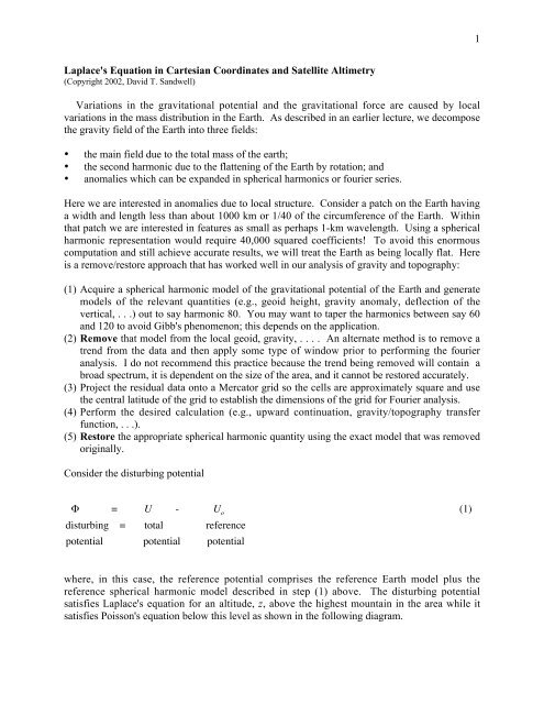
1Laplace's Equation in Cartesian Coordinates and Satellite Altimetry(Copyright 2002, David T. Sandwell)Variations in the gravitational potential and the gravitational force are caused by localvariations in the mass distribution in the Earth. As described in an earlier lecture, we decomposethe gravity field of the Earth into three fields:• the main field due to the total mass of the earth;• the second harmonic due to the flattening of the Earth by rotation; and• anomalies which can be expanded in spherical harmonics or fourier series.Here we are interested in anomalies due to local structure. Consider a patch on the Earth havinga width and length less than about 1000 km or 1/40 of the circumference of the Earth. Withinthat patch we are interested in features as small as perhaps 1-km wavelength. Using a sphericalharmonic representation would require 40,000 squared coefficients! To avoid this enormouscomputation and still achieve accurate results, we will treat the Earth as being locally flat. Hereis a remove/restore approach that has worked well in our analysis of gravity and topography:(1) Acquire a spherical harmonic model of the gravitational potential of the Earth and generatemodels of the relevant quantities (e.g., geoid height, gravity anomaly, deflection of thevertical, . . .) out to say harmonic 80. You may want to taper the harmonics between say 60and 120 to avoid Gibb's phenomenon; this depends on the application.(2) Remove that model from the local geoid, gravity, . . . . An alternate method is to remove atrend from the data and then apply some type of window prior to performing the fourieranalysis. I do not recommend this practice because the trend being removed will contain abroad spectrum, it is dependent on the size of the area, and it cannot be restored accurately.(3) Project the residual data onto a Mercator grid so the cells are approximately square and usethe central latitude of the grid to establish the dimensions of the grid for Fourier analysis.(4) Perform the desired calculation (e.g., upward continuation, gravity/topography transferfunction, . . .).(5) Restore the appropriate spherical harmonic quantity using the exact model that was removedoriginally.Consider the disturbing potentialΦ = U - U o(1)disturbing = total referencepotential potential potentialwhere, in this case, the reference potential comprises the reference Earth model plus thereference spherical harmonic model described in step (1) above. The disturbing potentialsatisfies Laplace's equation for an altitude, z, above the highest mountain in the area while itsatisfies Poisson's equation below this level as shown in the following diagram.

z2∆ 2 Φ = 0yair∆ 2 Φ = -4πGρrockxΦ(x,y,z) -- disturbing potential (total - reference)G -- gravitational constantρ -- density anomaly (total - reference)Laplace's equation is a second order partial differential equation in three dimensions.2 2 2∂ Φ ∂ Φ ∂ Φ+ + = 0, z > 0 (2)2 2 2∂x ∂y ∂zSix boundary conditions are needed to develop a unique solution. Far from the region, thedisturbing potential must go to zero; this accounts for 5 of the boundary conditionslim Φ= 0, lim Φ= 0, lim Φ= 0 (3)x →∞ y →∞ z→∞At the surface of the earth (or at some elevation), one must either prescribe the potential or thevertical derivative of the potential.Φ( xy , , 0) = Φ ( xy , ) - - Dirichleto∂Φ∂z= −∆gxy( , ) - - Neumann (4)To solve this differential equation, we'll use the 2-D fourier transform again where the forwardand inverse transform are∞ ∞∫ ∫−i2π( kx ⋅ ) 2F(k) = f( x)e d x (5)−∞ −∞∞ ∞∫ ∫i2π( kx ⋅ ) 2f(x) = F( k)e d k−∞ −∞

4The upward continuation physics is the same for the potential and all of its derivatives. Forexample, if one measured gravity anomaly at the surface of the earth ∆g(x,0), then to computethe gravity at an altitude of z, one takes the fourier transform of the surface gravity, multiplies bythe upward continuation kernel, and inverse transforms the result. This exponential decay of thesignal with altitude is a fundamental barrier to recovery of small-scale gravity anomalies from ameasurement made at altitude. Here are two important examples.i) Marine gravity - Consider making marine gravity measurement on a ship which is 4 km abovethe topography of the ocean floor. (Most of the short-wavelength gravity anomalies aregenerated by the mass variations associated with the topography of the seafloor.) At awavelength of say 8 km, the ocean surface anomaly will be attenuated by 0.043 from theamplitude of the seafloor anomaly.ii) Satellite gravity - The typical altitude of an artificial satellite used to sense variations in thegravity field is 400 km so an anomaly having a 100-km wavelength will be attenuated by a factorof 10 -11 ! This is why radar altimetry (below), which measures the geoid height directly on theocean surface topography is so valuable.Derivatives of the gravitational potentialThis solution to Laplace's equation can be used to construct all of the common derivatives ofthe potential. Suppose one has a complete survey over a patch on the surface of the earth so afourier method can be used to convert among the different representations of the gravity field.This is particularly true for computing gravity anomaly from geoid height or deflection of thevertical. The general relation between the potential in the space domain (at any altitude) and thefourier transform of the surface potential is.∞ ∞− k z i ( ⋅ )Φ( x, z) = ∫ ∫ Φ( k,0)e 2 π kxe 2 πd2 k−∞ −∞The following table uses equation (10) and the definitions of the derivatives of the potential toconstruct the variety of anomalies. Before examining these relationships however, lets reviewsome of the definitions in relation to what can be measured.(10)Gravitational potentialFirst derivative of potentialN - geoid height - Since the ocean surface is an equipotentialsurface, variations in gravitational potential will produce variationsin the sea surface height. This can be measured by a radaraltimeter.∆g - gravity anomaly - This is the derivative of the potential withrespect to z. It can be measured by an accelerometer such as agravity meter.η, ξ - deflection of the vertical - These are the derivatives of thepotential with respect to x and y, respectively. These are also

5forces, however, they are usually measured by recording the tinyangle between a plumb bob and the vector pointing to the center ofthe earth. Over the ocean this is most easily measured by takingthe along-track derivative of radar altimeter profiles.2 2 2⎡∂Φ ∂ Φ ∂ Φ ⎤⎢ 2∂x ∂∂ x y ∂∂ x z⎥⎢22 ⎥∂ Φ ∂ ΦSecond derivative of potential- ⎢⎥- gravity gradient - This is a symmetric2⎢ ∂y∂∂ y z ⎥⎢2∂ Φ ⎥⎢⎥2⎣⎢∂z⎦⎥tensor of second partial derivatives of the gravitational potential.A direct way of making this measurement is to construct a set ofaccelerometers each spaced at a distance of ∆ in the x, y, and zdirections. What is the minimum number of accelerometersneeded to measure the full gravity gradient tensor? What can yousay about the trace of this tensor when the measurements are madein free space? Below we'll develop an alternate method ofmeasuring ∂ 2Φover the ocean using a radar altimeter.2∂zTable 1. Relationships among the various representations of the gravity field in free space.space domainwavenumber domaingeoid height from thepotentialN( x) ≅ 1 Φ( x, 0)N( k) ≅ 1 Φ ( k, 0)(11)gggravity anomaly from thepotentialdeflection of the verticalfrom the potential (east slopeand north slope)Φ∆g( x, z) ≅− ∂ ( x, z)∂z∂N1 ∂Φη( x)=− ≅−∂x g ∂x∂N1 ∂Φξ( x)=− ≅−∂y g ∂y−2πz∆g( k, z) ≅ 2πkekΦ( k, 0)i2πkxη( k) ≅− Φ( k, 0)gi2πkyξ( k) ≅− Φ( k, 0)g(12)(13)gravity anomaly fromdeflection of the vertical[Haxby et al., 1983][ ]ig∆g( k) = kxη( k) + kyξ ( k)(14)kvertical gravity gradientfrom the curvature of theocean surface2 2∂g⎛ ∂ N ∂ N ⎞= g⎜+ ⎟ (15)2 2∂z⎝ ∂x∂y⎠

6As an exercise, use Laplace's equation and the various definitions to develop gravity anomalyfrom vertical deflection (equation 14) and vertical gravity gradient from ocean surface curvature(equation 15).Here is a practical example. Suppose one has measurements of geoid height N(x)over a largearea on the surface of the ocean and we wish to calculate the gravity anomaly, ∆g(x,z) at altitude.The prescription is:(1) remove an appropriate spherical harmonic model from the geoid;(2) take the 2-D fourier transform of Ν(x);−2πk(3) multiply by g2πk e ;(4) take inverse 2-D fourier transform;(5) restore the matching gravity anomaly calculated from the spherical harmonic model ataltitude.Conversion of geoid height to vertical deflection, gravity anomaly, and vertical gravitygradient from satellite altimeter profilesAs described above, geoid height N(x) and other measurable quantities such as gravityanomaly g(x) are related to the anomalous gravitational potential Φ(x,z) through Laplace'sequation. It is instructive to go through an example of how measurements of ocean surfacetopography from satellite altimetry can be used to construct geoid height, deflection of thevertical, gravity anomaly, and vertical gravity gradient.The surface of the ocean is displaced both above and below the reference ellipsoidal shape ofthe Earth (Figure 2). These differences in height arise from variations in gravitational potential(i.e., geoid height) and oceanographic effects (tides, large-scale currents, el Nino, eddies, . . .).Fortunately, the oceanographic effects are small compared with the permanent gravitationaleffects so a radar altimeter can be used to measure these bumps and dips. At wavelengths lessthan about 200 km, bumps an dips in the ocean surface topography reflect the topography of theocean floor and can be used to estimate seafloor topography in areas of sparse ship coverage.Radar altimeters are used to measure the height of the ocean surface above the referenceellipsoid (i.e., the satellite above the ellipsoid H * minus the altitude above the ocean surface H).A GPS, or ground-based tracking system, is used to establish the position of the radar H * (as afunction of time) to an accuracy of better than 0.1 m. The radar emits 1000 pulses per second atKu-band. These spherical wave fronts reflect from the closest ocean surface (nadir) and return tothe satellite where the two-way travel times is recorded to an accuracy of 3 nanoseconds (1-mrange variations mostly due to ocean waves). Averaging thousands of pulses reduces the noise toabout 30 mm. If one is interested in making an accurate geoid height map such, as shown inFigure 4, then many sources of error must be considered and somehow removed. However, ifthe final product of interest is one of the derivatives of the potential then it is best to take the

7along-track derivative of each profile to develop along-track sea surface slope. In this case, thepoint-to-point precision of the measurements is the limiting factor.Figure 2. Schematic diagram of a radar altimeter orbiting the earth at an altitude of 800 km.

8Figure 3. Ground tracks for two radar altimeters that have provided adequate coverage of the oceansurface. This is a 1500-km by 1000-km area around Hawaii. Geosat/ERM (US Navy) is the exact repeatorbit phase of the Geosat altimeter mission (US Navy, 1985-89). These ground tracks repeat every 17days to monitor small changes in ocean surface height caused by time-varying oceanographic effects.Geosat/GM ground tracks were acquired during a 1.5-year period when the orbit was allowed to drift.Similarly ERS/GM was a European Space Agency phase of the ERS mission that acquired non-repeatprofiles for 1 year. ERS/ERM is the 35-day repeat phase of the ERS mission.Figure 4. Geoid height above the WGS84 ellipsoid in meters (5-m contour interval) derived fromaltimeter profiles in Figure 3. The geoid height is dominated by long-wavelengths so it is difficult toobserve the small-scale features caused by ocean-floor topography. These can be enhanced by computingeither the horizontal derivative (ocean surface slope) or the vertical derivative ( gravity anomaly).To avoid a crossover adjustment of the data, ascending and descending satellite altimeterprofiles are first differentiated in the along-track direction resulting in geoid slopes or alongtrackvertical deflections. These along-track slopes are then combined to produce east η andnorth ξ components of vertical deflection [Sandwell, 1984]. Finally the east and north verticaldeflections are used to compute both gravity anomaly and vertical gravity gradient. Thealgorithm used for gridding the altimeter profiles is an iteration scheme that relies on rapidtransformation from ascending/descending geoid slopes to north/east vertical deflection and viceversa. The details for converting along-track slope into east and north components of deflectionof the vertical are provided in the Appendix and also in a reference [Sandwell and Smith, 1997].You probably don't need to know these details unless you plan to do research in marine gravity.

9Figure 5. East component of sea surface slope η(x) derived from Geosat and ERS altimeter profiles. Notethis component is rather noisy because the altimeter tracks (Figure 3) run mainly in a N-S direction.Figure 6. North component of sea surface slope ξ(x) derived from Geosat and ERS altimeter profiles.Note this component has lower noise because the altimeter tracks (Figure 3) run mainly in a N-Sdirection.To compute gravity anomaly (Figure 7) from a dense network of satellite altimeter profiles ofgeoid height (Figure 2), one constructs grids of east η and north ξ vertical deflection (Figures 5and 6). The grids are then Fourier transformed and Eq. (5) is used to compute gravity anomaly.At this point one can add the long wavelength gravity field from the spherical harmonic model to

10the gridded gravity values in order to recover the total field; the resulting sum may be comparedwith gravity measurements made on board ships. A more complete description of gravity fieldrecovery from satellite altimetry can be found in [Hwang and Parsons, 1996; Sandwell andSmith, 1997; Rapp and Yi, 1997].Figure 7. Gravity anomaly ∆g(x) derived from east and north components of sea surface slope usingequation (14). (50 mGal contour interval)Figure 8. Vertical gravity gradient dg(x)/δz derived from east and north components of sea surface slopeusing equation (15). Note this second derivative of the geoid amplifies the shortest wavelengths; comparewith the original geoid (Figure 3). Noise in the altimeter measurements has been amplified resulting in anartificial texture. (100 Eotvos contour interval)

11There is an important issue for constructing gravity anomaly from sea surface slope that isrevealed by a simplified version of equation (14). Consider the sea surface slope and gravityanomaly across a two-dimensional structure which depends on x but not y. The y-component ofslope is zero so conversion from sea surface slope to gravity anomaly is simply a Hilberttransform:∆g( k) igsgn( k)η k(16)= ( )x x xNow it is clear that one µrad of sea surface slope maps into 0.98 mGal of gravity anomaly andsimilarly one µrad of slope error will map into ~1 mGal of gravity anomaly error. Thus theaccuracy of the gravity field recovery is controlled by the accuracy of the sea surface slopemeasurement.APPENDIX - Vertical Deflections from Along-Track SlopesConsider for the moment the intersection point of an ascending and a descending satellitealtimeter profile. The derivative of the geoid height N with respect to time t along the ascendingprofile isN a ≡ ∂Na∂tand along the descending profile is= ∂N θ a + ∂N φ a∂θ ∂φ(B1)N d = ∂N∂θ θ d + ∂N∂φ φ d(B2)where is θ geodetic latitude and φ is longitude. The functions θ and φ are the latitudinal andlongitudinal components of the satellite ground track velocity. It is assumed that the satellitealtimeter has a nearly circular orbit so that its velocity depends mainly on latitude; at thecrossover point the following relationships are accurate to better than 0.1%.θ a = -θ d φ a = φ d (B3)The geoid gradient (deflection of the vertical) is obtained by solving (B1) and (B2) using (B3).

12∂N= 1 ∂φ 2φ∂N∂θ = 12θNa + N dNa - N d(B4)(B5)It is evident from this formulation that there are latitudes where either the east or northcomponent of geoid slope may be poorly determined. For example, at ±72˚ latitude, the Seasatand Geosat altimeters reach their turning points where the latitudinal velocity θ goes to zero andthus (B4) becomes singular. In the absence of noise this is not a problem because the ascendingand descending profiles are nearly parallel so that their difference goes to zero at the same ratethat the latitudinal velocity goes to zero. Of course in practice altimeter profiles contain noise, sothat the north component of geoid slope will have a signal to noise ratio that decreases near ±72˚latitude. Similarly for an altimeter in a near polar orbit, the ascending and descending profilesare nearly anti-parallel at the low latitudes; the east component of geoid slope is poorlydetermined and the north component is well determined. The optimal situation occurs when thetracks are nearly perpendicular so that the east and north components of geoid slope have thesame signal to noise ratio.When two or more satellites with different orbital inclinations are available, the situation isslightly more complex but also more stable. Consider the intersection of 4 passes as shown inthe following diagram.2 41 3The along-track derivative of each pass can be computed from the geoid gradient at the crossoverpoint

13N 1θ 1 φ 1∂NN 2=N 3N 4θ 2 φ 2θ 3 φ 3θ 4 φ 4∂θ∂N∂φ(B6)or in matrix notationN = Θ ∇N(B7)Since this is an overdetermined system, the 4 along-track slope measurements cannot be matchedexactly unless the measurements are error-free. In addition, an a-priori estimate of the error inthe along-track slope σ i measurements can be used to weight each equation in (B6) (i.e. divideeach of the four equations by σ i ). The least squares solution to (B7) is∇N = Θ t Θ -1 Θ t N(B8)where t and -1 are the transpose and inverse operations, respectively. In this case a 2 by 4system must be solved at each crossover point although the method is easily extended to three ormore satellites. Later we will assume that every grid cell corresponds to a crossover point of allthe satellites considered so this small system must be solved many times.In addition to the estimates of geoid gradient, the covariances of these estimates are alsoobtained2σ θθ2σ φθ2σ θφ2σ φφ= (Θ t Θ) -1 (B9)Since Geosat and ERS-1 are high inclination satellites, the estimated uncertainty of the eastcomponent is about 3 times greater than the estimated uncertainty of the north component at theequator. At higher latitudes of 60˚-70˚ where the tracks are nearly perpendicular, the north andeast components are equally well determined. At 72˚ north where the Geosat tracks run in awesterly direction, the uncertainty of the east component is low and the higher inclination ERS-1tracks prevent the estimate of the north component from becoming singular at 72˚.Finally, the east η and north ξ components of vertical deflection are related to the two geoidslopes by

14η = - 1 ∂Na cos θ ∂φ(B10)where a is the mean radius of the earth.ξ = - 1 a∂N∂θ(B11)REFERENCESHaxby, W. F., Karner, G. D., LaBrecque, J. L., and Weissel, J. K. (1983). Digital images ofcombined oceanic and continental data sets and their use in tectonic studies. EOS Trans.Amer. Geophys. Un. 64, 995-1004.Hwang, C., and Parsons, B. (1996). An optimal procedure for deriving marine gravity frommulti-satellite altimetry. J. Geophys. Int. 125, 705-719.Rapp, R. H., and Yi, Y. (1997). Role of ocean variability and dynamic topography in therecovery of the mean sea surface and gravity anomalies from satellite altimeter data. J.Geodesy 71, 617-629.Sandwell, D. T. (1984). A detailed view of the South Pacific from satellite altimetry. J.Geophys. Res. 89, 1089-1104.Sandwell, D. T., and Smith, W. H. F. (1997). Marine gravity anomaly from Geosat and ERS-1satellite altimetry. J. Geophys. Res. 102, 10,039-10,054.Yale, M. M., D. T. Sandwell, and W. H. F. Smith, Comparison of along-track resolution ofstacked Geosat, ERS-1 and TOPEX satellite altimeters, J. Geophys. Res., 100, p. 15117-15127, 1995.