Over-Soft Clay

More documents

Recommendations

Info

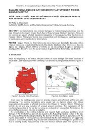
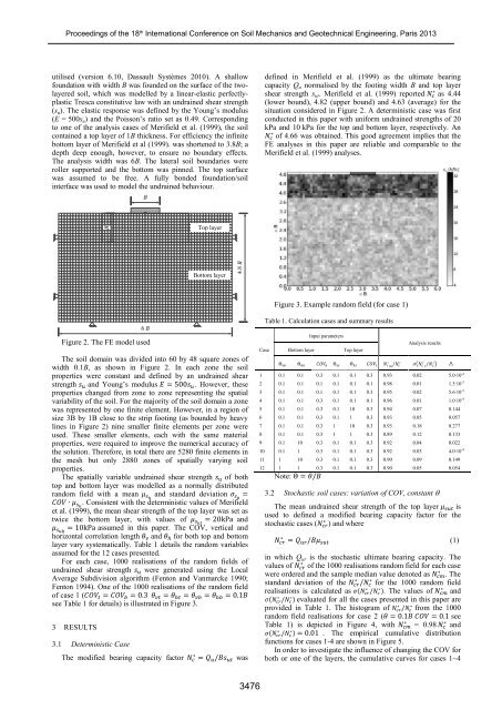
Proceedings of the 18 th International Conference on Soil Mechanics and Geotechnical Engineering, Paris 2013Proceedings of the 18 th International Conference on Soil Mechanics and Geotechnical Engineering, Paris 2013utilised (version 6.10, Dassault Systèmes 2010). A shallowfoundation with width B was founded on the surface of the twolayeredsoil, which was modelled by a linear-elastic perfectlyplasticTresca constitutive law with an undrained shear strength(s u ). The elastic response was defined by the Young’s modulus(E = 500s u ) and the Poisson’s ratio set as 0.49. Correspondingto one of the analysis cases of Merifield et al. (1999), the soilcontained a top layer of 1B thickness. For efficiency the infinitebottom layer of Merifield et al (1999). was shortened to 3.8B; adepth deep enough, however, to ensure no boundary effects.The analysis width was 6B. The lateral soil boundaries wereroller supported and the bottom was pinned. The top surfacewas assumed to be free. A fully bonded foundation/soilinterface was used to model the undrained behaviour.Bdefined in Merifield et al. (1999) as the ultimate bearingcapacity Q u normalised by the footing width B and top layershear strength s ut . Merifield et al. (1999) reported as 4.44(lower bound), 4.82 (upper bound) and 4.63 (average) for thesituation considered in Figure 2. A deterministic case was firstconducted in this paper with uniform undrained strengths of 20kPa and 10 kPa for the top and bottom layer, respectively. Anof 4.66 was obtained. This good agreement implies that theFE analyses in this paper are reliable and comparable to theMerifield et al. (1999) analyses.BTop layerBottom layer4.8 BFigure 3. Example random field (for case 1)6 BFigure 2. The FE model usedThe soil domain was divided into 60 by 48 square zones ofwidth 0.1B, as shown in Figure 2. In each zone the soilproperties were constant and defined by an undrained shearstrength and Young’s modulus . However, theseproperties changed from zone to zone representing the spatialvariability of the soil. For the majority of the soil domain a zonewas represented by one finite element. However, in a region ofsize 3B by 1B close to the strip footing (as bounded by heavylines in Figure 2) nine smaller finite elements per zone wereused. These smaller elements, each with the same materialproperties, were required to improve the numerical accuracy ofthe solution. Therefore, in total there are 5280 finite elements inthe mesh but only 2880 zones of spatially varying soilproperties.The spatially variable undrained shear strength of bothtop and bottom layer was modelled as a normally distributedrandom field with a mean and standard deviation. Consistent with the deterministic values of Merifieldet al. (1999), the mean shear strength of the top layer was set astwice the bottom layer, with values ofandassumed in this paper. The COV, vertical andhorizontal correlation length and for both top and bottomlayer vary systematically. Table 1 details the random variablesassumed for the 12 cases presented.For each case, 1000 realisations of the random fields ofundrained shear strength were generated using the LocalAverage Subdivision algorithm (Fenton and Vanmarcke 1990;Fenton 1994). One of the 1000 realisations of the random fieldof case 1 (see Table 1 for details) is illustrated in Figure 3.3 RESULTS3.1 Deterministic CaseThe modified bearing capacity factorwasCaseTable 1. Calculation cases and summary resultsBottom layerInput parametersTop layerAnalysis results( ) 1 0.1 0.1 0.3 0.1 0.1 0.3 0.93 0.02 5.0∙10 -42 0.1 0.1 0.1 0.1 0.1 0.1 0.98 0.01 1.3∙10 -33 0.1 0.1 0.1 0.1 0.1 0.3 0.95 0.02 5.6∙10 -34 0.1 0.1 0.3 0.1 0.1 0.1 0.96 0.01 1.0∙10 -45 0.1 0.1 0.3 0.1 10 0.3 0.94 0.07 0.1446 0.1 0.1 0.3 0.1 1 0.3 0.93 0.05 0.0577 0.1 0.1 0.3 1 10 0.3 0.93 0.18 0.2778 0.1 0.1 0.3 1 1 0.3 0.89 0.12 0.1339 0.1 10 0.3 0.1 0.1 0.3 0.92 0.04 0.02210 0.1 1 0.3 0.1 0.1 0.3 0.92 0.03 4.0∙10 -411 1 10 0.3 0.1 0.1 0.3 0.90 0.09 0.14912 1 1 0.3 0.1 0.1 0.3 0.90 0.05 0.054Note:3.2 Stochastic soil cases: variation of COV, constant The mean undrained shear strength of the top layer isused to defined a modified bearing capacity factor for thestochastic cases ( ) and wherein which Q ur is the stochastic ultimate bearing capacity. Thevalues of of the 1000 realisations random field for each casewere ordered and the sample median value denoted as . Thestandard deviation of the for the 1000 random fieldrealisations is calculated as ( ). The values of and( ) evaluated for all the cases presented in this paper areprovided in Table 1. The histogram of from the 1000random field realisations for case 2 (seeTable 1) is depicted in Figure 4, with = 0.98 and( ) . The empirical cumulative distributionfunctions for cases 1-4 are shown in Figure 5.In order to investigate the influence of changing the COV forboth or one of the layers, the cumulative curves for cases 1~4(1)3476
Technical Committee CFMS / Comité technique CFMSProceedings of the 18 th International Conference on Soil Mechanics and Geotechnical Engineering, Paris 2013are shown in Figure 5. In these cases the horizontal and verticalcorrelation lengths of both top and bottom layers were keptconstant as . As shown in the figure, the averagebearing capacity factor for all of the stochastic cases(represented by ) is less than the deterministic case. This isconsistent with the reports of Nobahar and Popescu (2000),Griffiths et al. (2002) and Cassidy et al. (2012). Further, whenthe COV of both layers is increased from 0.1 to 0.3 the averagebearing capacity reduces from 0.98 to 0.93 and the normalisedstandard deviation increases from 0.01 to 0.02. This is asexpected and is shown in the two extremity curves of Figure 5.Comparing the cases where the COV of only the top layer (case3: COV b =0.1, COV t =0.3) and only the bottom layer (case 4:COV b =0.3, COV t =0.1) provides more insight into themechanisms of failure. We can see from Figure 5 that the COVof the top layer has a more significant effect with case 3trending towards case 1 where both layers are 0.3. Moreover,the similarity of the shapes of case 2 and case 4 as well as case3 and case 1 implies that the top layer COV determines thevariation (standard deviation) of the curves.it provides a measure of the unconservatism in usingdeterministic bearing capacity factors, i.e., in neglectinguncertainty and spatial variability. In only 6 cases out of the 12analyzed, output samples resulted to be lognormal at the 95%confidence level using the Anderson-Darling test. Hence,estimating the probability of exceedence of unity fromcumulative values of fitted lognormal samples would not allowconfident assessement for all cases. Empirical cumulativedistribution functions were calculated for each sample. Theempirical probability P e of exceedence of unity for each case isnoted in the rightmost column in Table 1.The failure mechanisms of three selected realizations of case1 ( ) are shown in Figure 6. Theserepresent the minimum, median and maximum cases andare shown alongside the deterministic failure mechanism(uniform and mean parameter values). In all three cases theexistence of the random field results in a non-symmetric failuremechanism, with the minimum bearing capacity case mostunsymmetrical. With the increasing of bearing capacity, thefailure mechanism tends to resemble the deterministic case. Theimportance of spatial variability in the top layer can beobserved, with the majority of the failure mechanism residing inthat layer. Further, with higher variability and potential forweaker zones the mechanism for lower bearing capacity is bothmore unsymmetric and shorter (pulling it further into the toplayer).(a)(b)Figure 4 Histogram of for case 2(c)(d)Figure 6. Failure mechanisms from finite element analysis for(a) lowest, (b) median and (c) highest bearing capacity, and (d)deterministic uniform case (for clarity only a section of 3Bwidth and depth 2B show)Figure 5 Cumulative probability curves for varying COV ofcases 1 to 4The output samples of stochastic bearing capacity factornormalized by the deterministic value were analysed with theaim of estimating the frequentist probability of exceedence ofunity, i.e., the probability that the stochastic bearing capacityfactor exceeds the deterministic bearing capacity factor. Thisassessment is important in the context of engineering design, as3.3 Stochastic soil cases: variation of correlation length intop layerWith the top layer determined to play a more significant rolein the problem configuration of this paper further concentrationon the effect of top layer correlation length is discussed. Theresults for correlation length varying from 0.1B to 10B arepresented as cumulative probability curves in Figure 7. Theserepresent cases 5, 6, 1, 7 and 8 in Table 1. As for thecases (cases 5, 6 and 1), the largest bearing capacitycorresponds to the largest horizontal correlation length(case 5) while the minimum corresponds to(case 6). This is consistent with the observation of Griffiths etal. (2002) for the single layer case. In general, a largecorrelation length results in greater standard deviation of thebearing capacity, i.e. the foundation becomes more “non-3477
Page 4: Proceedings of the 18 th Internatio

Over-Soft Clay

You also want an ePaper? Increase the reach of your titles

Delete template?

Save as template?