Phthalates and Nonylphenols in Roskilde Fjord

[Blank page]

Ministry of Environment and EnergyNational Environmental Research InstituteThe Aquatic EnvironmentPhthalates andNonylphenolsin Roskilde FjordA Field Study and Mathematical Modellingof Transport and Fate in Water and SedimentNERI Technical Report No. 339February 2001Jørgen VikelsøePatrik FauserPeter B. SørensenLars CarlsenDepartment of Environmental Chemistry

Data sheetTitle:Phthalates and Nonylphenols in Roskilde FjordSubtitle:A Field Study and Mathematical Modelling of Transport and Fate in Water andSediment. The Aquatic EnvironmentAuthorsJørgen Vikelsøe, Patrik Fauser, Peter B. Sørensen & Lars CarlsenAnalytical laboratory:Elsebeth JohansenDepartment:Department of Environmental ChemistrySediment samples:Rikke HansenSerial title and no.: NERI Technical Report No. 339Publisher:Ministry of Environment and EnergyNational Environmental Research Institute ©URL:http://www.dmu.dkDate of publication: February 2001Referee:Henrik Søren Larsen, Danish Environmental Protection AgencyLayout:Jørgen Vikelsøe, Patrik Fauser & Majbritt Pedersen-UlrichPlease cite as:Vikelsøe, J., Fauser, P., Sørensen, P.B. & Carlsen, L. (2001): Phthalates and Nonylphenolsin Roskilde Fjord. A Field Study and Mathematical Modelling of Transportand Fate in Water and Sediment. The Aquatic Environment. National EnvironmentalResearch Institute, Roskilde. 106pp. NERI Technical Report. No. 339Reproduction is permitted, provided the source is explicitly acknowledged.Abstract:The aim of the study has been to investigate the occurrence, sources, transport andfate of nonylphenols and phthalates in the aquatic environment of Roskilde Fjord. Itwas further intended to find the temporal as well as the spatial variation of these xenobioticsin the fjord and stream water. Further, to investigate nonylphenols andphthalates in sediment in the fjord including a sediment core in the southern part, expectedto yield clues regarding the historical variation of the concentration of xenobiotics,as well as some streams and lakes. Finally, an important aim was to make amass balance for the fjord system, including sources, transport and the mechanismsof elimination, and to make a mathematical model describing the fate of the substancesin the fjord system.Keywords:Phthalates, PAE, Nonylphenols, NPE, DEHP, analysis, estuary, fjord, water, sediment,mathematical model, mass balance.ISBN: 87-7772-585-9ISSN (print): 0905-815XISSN (electronic): 1600-0048Paper quality and print: Cyclus Office, 100 % recycled paper. Grønager’s Grafisk Produktion AS.This publication has been marked with the Nordic environmental logo "Svanen".Number of pages: 106Circulation: 200Price:DKK 75,- (incl. 25% VAT, excl. freight)Internet-version:The report is also available as a PDF-file from NERI’s homepageFor sale at:2National Environmental Research InstitutePostboks 358Frederiksborgvej 399DK-4000 RoskildeTel.: +45 46 30 12 00Fax: +45 46 30 11 14MiljøbutikkenInformation and BooksLæderstræde 1DK-1201 Copenhagen KDenmarkTel.: +45 33 95 40 00Fax: +45 33 92 76 90e-mail: butik@mem.dkwww.mem.dk/butik

ContentsSummary 5Resumé 71 Introduction 92 Purpose 113 Experimental 133.1 Monthly samples of fjord water 133.2 Seasonal sampling plan 133.3 Samples of fjord sediment 164 Analytical 194.1 Sampling 194.2 Extraction of water samples. 204.3 Extraction of sediment samples 204.4 Blanks 204.5 Standards and spikes 214.6 Gaschromatography/mass spectrometry (GC/MS) 224.7 Performance test of analytical method for water 224.8 Performance test of sediment method 245 Results and statistics 275.1 Fjord water 275.1.1 Abundance of substances 275.1.2 Temporal and spatial variation 285.1.3 Monthly samples in Roskilde Vig and Bredning 325.1.4 Analysis of variance 345.1.5 Discussion 345.1.6 Analysis of correlation 355.2 Fjord sediment 395.2.1 Abundance of substances 395.2.2 Horizontal distribution 405.2.3 Vertical distribution in sediment core 435.3 Streams and lake 455.3.1 Water 455.3.2 Sediment 485.3.3 Correlation analysis of streams and lake 515.4 Deposition 526 Mathematical data interpretation 556.1 Physico-chemical processes 556.1.1 Microbial degradation 566.1.2 Sorption and solvation 576.1.3 Sedimentation 586.1.4 Vertical transport in the sediment 616.1.5 Horizontal transport in the water 633

6.2 Sources 646.3 Model parameters 656.4 Model set-up 666.4.1 Steady-state box-model 686.4.2 Numerical models (water and sediment model) 686.4.3 Dynamic solution to the diffusion and sedimentationproblem in the sediment 736.4.4 Steady-state solution to the diffusion, sedimentationand degradation problem in the sediment 736.5 Discussion of experimental and analytical results in thesediment 746.6 Discussion of experimental and analytical results in thewater compartment 777 Conclusions 818 References 839 Abbreviations 8710 Variables 8911 Acknowledgements 9312 Appendix A. Analytical performance test 9512.1 Detection limits 9512.2 Figures, method for water 9612.2.1 Linearity of method for water 10012.3 Figures, method for sediment 10112.3.1 Linearity of method for sediment 104National Environmental Research Institute 105NERI Technical Reports 1064

SummaryThe occurrence sources, transport and fate of nonylphenols and phthalatesin the aquatic environment of a fjord was investigated. The substancesanalysed were: NP, NPDE, DBP, DPP, BBP, DEHP, DnOP andDnNP. The analytical methods were specifically developed for the investigation,using high resolution GC/MS. The investigation comprisedmeasurements of water and sediment in the fjord as well as in sources.The level and the temporal and spatial variation of the xenobiotics in thewater of the fjord were studied during three seasonal campaigns, involvingwidespread different locations. Very low concentrations were found.DEHP was the most abundant substance, followed by much lower concentrationsof DBP, BBP, DPP and NP. NPDE was not found. The concentrationsof the higher phthalates were highly significantly intercorrelated.On a large geographical scale the spatial variation was insignificant,but a significant seasonal variation was present, indicated by amaximum for June and a minimum for December, confirmed by analysisof variance. The largest seasonal variation and a significant short-termvariation were present at the narrow middle location, where the currentvelocity is high. The broad innermost part, near Roskilde, was most constant.Sediment was investigated in the innermost part of the fjord (RoskildeVig). Much higher concentrations were found than in the water, DEHP,DBP NP and NPDE being most abundant. A decreasing gradient fromthe WWTP outlet to a location 6 km away was observed, approaching theconcentrations found in the other less polluted fjord, Isefjord. Thus, horizontaltransport through the water is limited to some kilometres, and themain transport process seems to be sedimentation, or binding to sedimentin the fjord bottom.The sediment investigation including a core 22 cm deep (~80 y old) fromRoskilde Vig. A decreasing tendency with depth/age was observed forDEHP and BBP, reflection the historical development in consumption ofphthalates. For NP and NPDE, a more complicate pattern was found,characterised by low concentrations in the upper/youngest part and twodeeper maxima, probably caused by variation in the use of NPEs .The seasonal sampling further comprised three streams and a lake, includingwater and sediment. In the water of the streams, the DEHP concentrationsranged up to the triple of the fjord. The spatial and temporalvariations were more pronounced and random, certainly because thestreams - unlike the fjord - are hydraulic and geographic separate entitieshaving different sources and flows. The lake sediment indicated a significantsedimentation of all substances – in particular NP and NPDE –in the deepest part of the lake.Numerical models were set up in order to describe the fate of the substancesin the water and sediment compartments of the fjord. Only DEHPdata was used since DEHP was the most abundant substance and the onlyone to occur in concentrations that are of environmental significance.5

The physico-chemical processes in the fjord that were considered to influencethe fate of DEHP, were: 1 st order degradation of dissolvedDEHP, adsorption to particulate matter, sedimentation of particulatematter, vertical diffusion in the sediment and dispersive mixing in thewater. DEHP sources to the fjord were streams, wastewater treatmentplant discharges and atmospheric deposition. Water exchange with thesurrounding sea removes DEHP, since the DEHP concentrations is negligiblein the sea.In order to establish a simple robust model, the seasonal variations werenot considered. More data concerning the growth and wilting cycle of thevegetation and the influence of changing emission patterns from consumersand wastewater treatment plants were needed and therefore meanannual conditions were simulated based on constant flows and concentrations.The numerical models were validated with analytical expressions. Theexperimental sediment core data was used to calibrate the sedimentmodel yielding a sedimentation rate of 2.5 mm pr. year, correspondingwell to a rate previously found for the fjord. Furthermore a distributioncoefficient equal to 10000 litre pr. kg dm and a 1 st order degradation rateof 2 ⋅ 10 -5 sec -1 were found.The sediment simulations showed that it is the sedimentation process thatgoverns the vertical transport of substance in the sediment. Diffusion isonly significant in the theoretical upstart of the system, where the concentrationgradient is large at the surface. This fact has further been investigatedin Sørensen et al. (2000), in relation to evaluating the genericcompartment model, SimpleBox, comprised in the European Union Systemfor the Evaluation of Substances, EUSES.The water model was made by dividing the fjord into two sections of totalmixing along the horizontal axis, where the surface areas were largeand into a narrow dispersive section where the horizontal flow was high.The shallow water was considered to be totally mixed along the verticalaxis in the whole fjord. The experimental water concentrations were approximatelyconstant only displaying minor spatial variations that couldnot be modelled, probably because of short-term effects such as tidalflow. The mean experimental concentration was a factor of 5 higher thanthe mean calculated concentration.Freshwater from streams were the predominant DEHP source to thefjord, followed by atmospheric deposition and wastewater treatmentplants. Sedimentation was the predominant removal mechanism followedby water exchange with the sea and degradation.In spite of the deviation between the experimental and calculated DEHPconcentrations in the water, the used modelling approach is considered tosimulate the complex interactions that take place in a system such as RoskildeFjord, satisfactorily. However, in order to employ the model as arisk assessment tool it is necessary to further investigate analytical detectionlimits, source contributions and temporal variations of the system.6

ResuméForekomst, kilder, transport og skæbne af nonylphenoler og phthalater idet akvatiske miljø af Roskilde Fjord blev undersøgt.Der blev analyseret for stofferne NP, NPDE, DBP, DPP, BBP, DEHP,DnOP og NP. De analytiske metoder var udviklet specielt for undersøgelsen,og anvendte højtopløsende GC/MS. Undersøgelsen omfattedemålinger af vand og sediment i fjorden samt kilder.Forekomst og variation i tid og rum af de miljøfremmede stoffer blev undersøgti tre årstid prøvetagninger, der omfattede lokaliteter vidtstraktlangs fjorden. Der blev fundet meget lave koncentrationer i fjordvandet.DEHP forekom i højest koncentration, fulgt af DBP i meget lavere koncentration,og minimale mængder af BBP, DPP og NP. NPDE kunne ikkepåvises. Der var en højsignifikant korrelation mellem de højerephthalater. I geografisk stor skala var de rumlige variationer ikke signifikante,men der var en signifikant årstidsvariation tilstede, kendetegnetved et maksimum i juli og et minimum i december, bekræftet ved variansanalyse.Den største variation og en betydelig korttidsvariation fandtesi den snævre midterste sted, hvor strømningshastigheden er høj. Deninderste del, nær Roskilde, var mere konstant.Der blev undersøgt sediment i den inderste del af fjorden (Roskilde Vig).Her fandtes meget højere koncentrationer end i vandet, idet DEHP, DBP,NP og NPDE var mest forekommende. En aftagende gradient fandtes fraudløbet af rensningsanlægget til en position i 6 km afstand, hvor koncentrationennærmede sig koncentrationen i Isefjorden, der anses for mindreforurenet. Horisontal transport gennem vandet er således begrænset tilnogle få kilometer, og hovedtransportprocessen synes at være sedimentation,eller binding til sediment på fjordbunden.I sedimentundersøgelsen indgik en kærne 22 cm dyb (ca. 80 år gammel)fra Roskilde Vig. I denne sås en aftagende koncentration med dybde/alderaf DEHP og BBP, hvilket afspejler den historiske udvikling iforbruget af phthalater. For NP og NPDE blev fundet et mere kompliceretmønster, kendetegnet ved to dybere maxima, som formentlig er forårsagetaf ændringer i forbruget af NPE.Årstids prøvetagningen omfattede tillige vand og sediment i tre åer og ensø. I åvandet gik DEHP koncentrationen op til det tredobbelte af fjordvandet.Variationerne i tid og sted var mere udtalte og tilfældige, hvilketkunne forventes fordi åerne i modsætning til fjorden er hydraulisk og geografiskadskilte enheder med forskellige kilder og strømning. Søsedimentetantydede en betydelig sedimentation af alle stoffer – særlig NP ogNPDE – i den dybeste del af søen.Numeriske modeller blev lavet med det formål, at beskrive skæbnen afstofferne i henholdsvis fjordens vand og sediment. Det var kun DEHPkoncentrationerne der var tilstrækkeligt høje til at have miljømæssig betydningog derfor blev disse kun anvendt.7

De fysisk-kemiske processer i fjorden, der ansås at være af betydning forDEHP’s skæbne, var: 1 ste ordens nedbrydning af opløst DEHP, adsorptiontil partikulært materiale, sedimentation af partikler, vertikal diffusion isediment og dispersiv opblanding i vandfasen. DEHP kilder til fjordenvar åer og vandløb, rensningsanlæg og atmosfærisk deposition. Vandudvekslingmed havet (Kattegat) fjernede DEHP, da koncentrationerne varubetydelige i havet.For at kunne fastlægge en simpel og robust model blev der ikke tagethøjde for de tidslige variationer i systemet. En større mængde data omkringplanters og dyrs vækstcyklus og betydningen af skiftende emissionerfra såvel forbrugere som rensningsanlæg ville være nødvendigt i denhenseende. Derfor blev årsmiddelværdier med konstante vandmængderog koncentrationer anvendt.De numeriske modeller blev valideret med analytiske udtryk. De eksperimentelledata for sedimentkernen blev brugt til at kalibrere sedimentmodellen, hvilket gav en sedimentationsrate på 2.5 mm pr. år, som svaredegodt til tidligere undersøgelser for fjorden. Derudover blev der fundeten fordelingskoefficient på 10000 liter pr. kg tørstof og en 1 ste ordensnedbrydningsrate på 2 ⋅ 10 -5 sek -1 .Sediment beregningerne viste, at sedimentationsprocessen er bestemmendefor den vertikale transport af stof i sedimentet. Diffusion er kunbetydende i den teoretiske opstartsfase af systemet, hvor koncentrationsgradientenved sedimentoverfladen er meget stor. Dette er undersøgtyderligere i Sørensen et al. (2000), i forbindelse med en evaluering afden generiske compartmenmodel, SimpleBox, som indgår i ”EuropeanUnion System for the Evaluation of Substances, EUSES”.Vandmodellen blev lavet ved at inddele fjorden i to dele med fuldstændigopblanding, hvor overfladearealet var stort og i en smal passage med dispersion,hvor den horisontale vandstrømning var høj. Den lavvandedefjord ansås at være fuldstændigt opblandet i dybden. De eksperimentellevandkoncentrationer var tilnærmelsesvist konstante og udviste kun mindrevariationer som funktion af stedet. Disse blev ikke modelleret, da desandsynligvis skyldtes korttids effekter såsom tidsvandsstrømninger. Dengennemsnitlige eksperimentelle koncentration var en faktor 5 højere endden gennemsnitlige beregnede koncentration.Ferskvand fra vandløb og åer var den dominerende DEHP kilde, efterfulgtaf atmosfærisk deposition og rensningsanlæg. Sedimentation varden dominerende fjernelsesmekanisme, efterfulgt af vandskifte med havetog nedbrydning.På trods af afvigelsen mellem de eksperimentelle og beregnede DEHPkoncentrationer i vandet, må den opstillede model anses for at simulerede komplekse interaktioner i Roskilde Fjord tilfredsstillende. For at anvendemodellen som et risikovurderingsværktøj vil det imidlertid værenødvendigt at undersøge forhold omkring detektionsgrænser for de betragtedestoffer samt kildetilførsler og tidslige variationer mere indgående.8

1 IntroductionThe finding of octyl-phthalates in wastewater at high concentrations severalyears ago (Miljøstyrelsen 1994) caused considerable concern, becausesome phthalates just by then had been recognised as possibly oestrogen-likeor carcinogenic, making them harmful to human health. Sincethen, many investigations of Danish waste water and sewage sludge haveconfirmed the presence of phthalates, (PAE) as well as nonylphenolethoxylates(NPEs), PAHs and an array of other pollutants. The emissionof chemicals into the environment leads to the risk of human exposure.The most severe effects ascribed to oestrogen-like substances seem onthe human reproductive health, causing reduced sperm quality and testicularcancer in men, and breast cancer in as well men as women (andother forms of cancer). Although the oestrogen-like effects for the nonylphenolsand phthalates are weak compared to many other substances andto oestrogen itself, the concentrations of these compounds in wastewaterare high compared to other xenobiotics (Toppary et al. 1995). Hence,nonylphenols and phthalates presumably play a significant role for thetotal oestrogen-like effect of sludge and wastewater.This line of thought initiated a series of investigations of the sources,transport and fate of xenobiotics, sponsored by the Danish EnvironmentalProtection Agency (DEPA), carried out by NERI. These investigationwere limited to the local community of Roskilde city and surroundings.The present investigation is a part of the series.In the previous investigations of the project, the emissions to wastewaterfrom an array of pre-selected industries and institutions pre-selectedsources were studied. The deposition of nonylphenols and phthalates wasmeasured in a nearby ground station, assumed to represent the fjord surfacereasonably well. Also, nonylphenols and phthalates in some streamswere investigated (Vikelsøe et al. 1998). However, in that study onlyabout one tenth of the total sources for wastewater was found. The substancesare to a large extent removed from wastewater by wastewatertreatment plants (WWTPs), but nevertheless some residual substancesremain in the outlet. This has been measured in connection with thesource project, and again in the WWTP modelling project (Fauser et al.2000).The present investigation sets the focus on Roskilde Fjord as a recipientof NPE and PAE, involving sources, transport and fate. It continues theabove mentioned source study, and includes measurements of the fjordwater itself. The sources of relevance for the fjord are the wastewatertreatment plan outlet, the deposition, and some small streams runninginto the fjord. Furthermore, sediment from the fjord is investigated, sincesediments play an important role in the transport and fate of xenobioticsin the aquatic environment of the fjord.9

2 PurposeThe aim of the study has been to investigate the occurrence, sources,transport and fate of nonylphenols and phthalates in the aquatic environmentof Roskilde Fjord. It was further intended to find the temporal aswell as the spatial variation of these xenobiotics in the fjord and streamwater. Further, to investigate nonylphenols and phthalates in sediment inthe fjord including a sediment core in the southern part, expected to yieldclues regarding the historical variation of the concentration of xenobiotics,as well as some streams and lakes. Finally, an important aim was tomake a mass balance for the fjord system, including sources, transportand the mechanisms of elimination, and to make a mathematical modeldescribing the fate of the substances in the fjord system.11

3 Experimental3.1 Monthly samples of fjord waterMonthly water samples were taken at two locations, one in the Southernpart (Roskilde Vig) near the city of Roskilde, and one further North (RoskildeBredning). County of Roskilde Authority took these samples froma boat, as an extension of the routine fjord-monitoring program, Table 1.Table 1 Monthly water samples taken in the southern part of Roskilde Fjord 1998Location Dir Sampling dates(station)24 21 19 23 16 18km Mar Apr May Jun Jul AugRoskilde Vig (St. 2) N 2 W W W W W W W W WRoskilde Bredning (St. 60) N 7 W W W W W W W W W WDir = direction and distance from Roskilde Harbour W = water sample6Oct19Oct20Nov21Dec3.2 Seasonal sampling planFurthermore, the experimental plan involved three seasonal samplingcampaigns, shown in overview in Table 2. Each campaign comprisedsampling of fjord water at the mouth of the fjord and at a narrow and abroader place at the middle. These samples were taken from the beach, abank or a bridge. In the June sampling session, some samples were takenthe same day with a time interval of 6 hours, corresponding to differenttide, and hence current direction in the narrowest part of the fjord. Ineach seasonal campaign, water samples were further taken in a brook(Helligrenden), two streams (Maglemose Å and Hove Å) and a lake(Gundsømagle Sø), which Hove Å flows through. In Hove Å and GundsømagleLake, some sediment samples were also taken. The lake is involvedin the Danish national monitoring program, NOVA.Table 2 Seasonal sampling, overviewLocation Type Dir Sampling dateskm Mar 98 Jun 98 Sep 98 Dec 98 Nov 99Skuldelev Fjord N 16 W W WFrederiksund Fjord N 21 W * W WKulhuse (mouth of fjord) Fjord N 37 W * W WHelligrenden mouth Brook E 12 W W W WMaglemose Å mouth Stream N 7 W WHove Å upstream lake Stream W S W W W SLake Gundsømagle Lake W W S W W S W SHove Å mouth Stream N 8 W W S W W SW = water S = sediment * Sampled twice with 6 hours interval13

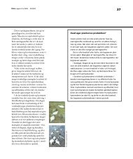
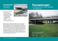
In Table 3 the flow in the streams 1998 on the sampling dates as well asthe monthly means are given according to hydrometric information fromRoskilde County (1999).Table 3 Flow in streams 1998Flow l/s Jan Feb Mar Apr May Jun Jul Aug Sep Oct Nov DecHove Å ups S 52.7 41.0 313M 243 368 438 464 135 48.3 64.0 57.5 45.1 138 363 373Hove Å dns S 510 54.2 41.0 774M 239 389 621 585 141 42.6 69.6 59.0 36.3 83.0 577 552Maglemose Å S 117 34.2M 86.6 149 212 230 36.7 16.4 35.1 29.0 13.3 70.1 124 148Helligrenden S 71.4 11.0 4.0 48.8M 62.0 82.4 93.6 99.8 25.9 11.1 9.2 5.8 4.0 29.9 45.9 66.9S = Sampling day M = Month mean ups = upstream the Lake dns = downstreamThe sampling locations are shown on the overview map in Figure 1.14

KulhuseSkuldelevRoskilde BredningGundsøHove ÅMaglemose ÅLille ValbyBramsnæsTempelkrogRoskilde VigHelligrenden).Figure 1Map in scale 1/200,000 showing the sampling locations.(Colour of circles: Fjord blue, streams and lake red, deposition black15

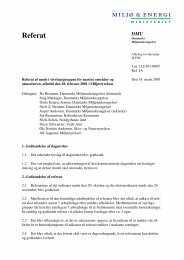
3.3 Samples of fjord sedimentFinally, sediment samples in the fjord was taken during 1996, most ofthem in Roskilde Vig in a fan-shaped geometry near the outlet from RoskildeWWTP (map Figure 2).NSludgeamendedfieldStation 2Roskilde Vig⊗∆WWTP outletFigure 21 kmRoskildeharbourLocal map of Roskilde Vig, 1:25000, showing locations of sedimentsampling sites and sources.x Sampling sites ⊗ Sediment core∆ WWTP outlet ∇ Sludge dumping site∇Roskilde CityThe sampling design is based on investigations carried out 1994-95 forRoskilde County Authority and Roskilde Municipality by Danish HydraulicInstitute and Water Consult. According to these reports the currentis circulating in the Vig mainly driven by the wind, the tide playing aminor role. The wind is predominantly in the West direction, leading toan South-East water current in the area having a velocity of 2-6 cm/sec.The WWTP average outlet of waste water is 19000 m 3 /day.Some samples were taken further North in Roskilde Vig and in RoskildeBredning, on the same locations as the monthly water samples. Thesediment also included samples from the neighbouring fjord Isefjord, believedto be lesser polluted, for comparison. These fjord sediment sampleswere taken by a diver. All sediment samples were taken in the upper2-5 cm of the sediment, with the exception of the core, which reached adepth of about 22 cm into the sediment. An overview of these samples isshown in Table 4.16The sampling methods are described more detailed in the AnalyticalChapter.

Table 4 Overview of samples of fjord sediment taken 1996Location Dir, km nRoskilde Vig, near WWTP outlet E 1 * 13Roskilde Vig, Station 2 N 2 1Roskilde Vig, Station 2044 N 4 1Roskilde Bredning, Station 60 N 6 1Isefjord, Tempelkrog & Bramsnæs 2Dir = direction and distance from Roskilde n = number of samples* including the core, counted here as one sample.17

4 AnalyticalThe following substances were analysed:NP, NPDE, DBP, DPP, BBP, DEHP, DnOP and DnNP.The analytical methods used are improvement of the methods used in theprevious parts of the project for water and soil (Vikelsøe et. al. 1998 &1999). A general problem encountered during analysis of phthalates islaboratory contamination, especially with DBP and DEHP, leading to ahigh analytical background (blank). The high background level impairsthe precision of the analysis and elevates the limits of determination,which is a particularly severe problem for samples in very low concentrations,such as the fjord water. As shown in the previous studies, themain cause for this is contaminated glassware. Hence, exclusively newglassware, annealed at 450°C, was used for sampling and laboratory procedures.All solvents used were HPLC grade.4.1 SamplingThe water was sampled in 2 l glass bottles, fastened in a special bottleholder mounted on a 3 m long pole. During sampling, the bottle mouthwas kept upstream, and the bottle was rinsed twice in the water beforethe final sampling. During boat sampling, the boat was sailing slowlyforward, and the sample taken near the prow. After the sampling, thevolume was adjusted to about 1.2 l. The sample was frozen in the bottlein horizontal position, and stored in the bottles.The sediment in the streams and the lake were sampled in new annealedthick-walled 1 l glass beakers fastened in a specially made beaker holdermounted on the pole. The bottom was scraped horizontally until thebeaker was filled. The samples were stored in the beakers, covered withaluminium foil.A diver sampled the fjord sediment, using stainless steel tubes 6.5 cm ininternal diameter, reaching about 5 cm into the fjord bottom, and disregardingsand. These samples were transferred to glass bottles with screwcaps for storage. The fjord sediment core 21 x 6.5 cm was sampled byhammering the stainless steel tube into the fjord bottom. It was stored inthe steel tube.All samples were frozen and stored at -20°C prior to analysis.Before analysis, the fjord sediment core was carefully removed from thesteel tube in the frozen state, and sawed in sections by means of sawblades cleaned by solvent rinsing. The operation was performed in thefreezing room. The sections were 0.5 cm high for the upper 10 cm, and 1cm sections for the lower 10 cm. The sediment was very hard, and difficultto slice. The uppermost 2 cm, which had a loose sandy texture, couldnot be sliced and was treated as an entity.19

4.2 Extraction of water samples.The water samples and their sampling bottles was treated as entities,since there may be a significant adsorption to the glass walls. Hence, itwas not allowed to divide the samples, or to take subsamples. Afterthawing at room temperature, the volume of water present in the samplingbottle was measured. A volume of 0.1 ml extraction spike solutioncontaining 0.1 µg of three deuterium labelled phthalates (Table 5) wasadded, the bottle was shaken and left for 15 min to equilibrate the extractionspikes with the water and the glass surfaces. The sample was extractedby shaking 5 min with 100 ml CH 2 Cl 2 after addition of 2 ml 5MHCl. When the phases were separated, a sub-extract of 50 ml was taken,concentrated to near dryness by evaporation and the remanence dissolvedin 0.1 ml syringe spike solution (Table 6) containing 0.1 µg D 4 -DnOP.4.3 Extraction of sediment samplesAfter thawing at laboratory temperature the samples were air-dried for 48hours on filter paper. About 5 g of dried sample was weighed accuratelyinto a 250 ml wide-necked Pyrex bottle. A volume of 0.1 ml extractionspike solution (Table 5) was added, distributed in the sample by shakingand left for 15 min to equilibrate the extraction spikes with the sampleand the glass surfaces, and allow the ethanol in the spike solution toevaporate. A volume of 100 ml dichloromethane was added, and the bottlewas closed by a screw-lid covered by aluminium-foil. The sample wasextracted at laboratory temperature by shaking for 4 hours in a shakingapparatus (Heidolph Unimax 2010 at 200 shakes/min). When the phaseswere separated, a sub-extract of 10 ml was concentrated by carefulevaporation under N 2 , and the remanence re-dissolved in a volume of 1ml syringe spike solution, Table 6.The extracts were analysed directly by high-resolution GC/MS withoutfurther clean up. If necessary, the samples were diluted appropriatelywith syringe spike solution.All sediment samples were extracted and analysed in duplicates.4.4 BlanksEvery day empty laboratory glassware was extracted for determination ofthe blank values, i.e. one blank for about every 10 samples. Care wastaken to treat the blanks in any way as samples, using same batches ofsolvents, glassware etc. The blanks were subtracted from the results onan amount per sample basis for each analytical series.20

4.5 Standards and spikesThe labelled spikes are used for identification, quantification and for calculationof the extraction recovery. Extraction spikes are added beforethe extraction, syringe spikes before GC/MS analysis.Table 5 Extraction spike solutionSubstance Acronym Label Waterµg/mlDibutylphthalateD 4 -DBPBenzylbutylphthalateD 4 -BBPDi-(2-ethylhexyl)phthalate D 4 -DEHPn-HexaneSolventSedimentµg/mlD 4 1.0 10Table 6 Syringe spike solutionSubstance Acronym Label Waterµg/mlSedimentµg/mlDi(n-octyl)-phthalate D 4 - DnOP D 4 1.0 0.1n-HexaneSolventStandard solutions are used for quantification and identification (Table 7)analysed by GC/MS for about every 5 samples.Table 7 Phthalate standard solutions for GC/MSSubstance Acronym Type µg/mllowNonylphenolNPStandard0.01Nonylphenol diethoxylate NPDE-0.05Di(n-butyl)phthalateDBP-0.01DipentylphthalateDPP-0.01D 4 -DibutylphthalateD 4 -DBP Extraction spike 0.1BenzylbutylphthalateBBP Standard0.01D 4 -Benzylbutylphthalate D 4 -BBP Extraction spike 0.1Di-(2ethylhexyl)-phthalateDi-(n-octyl)-phthalateDi-(n-nonyl)-phthalateD 4 -Di-(2ethylhexyl)-phthalateDEHPDnOPDnNPD 4 -DEHPStandard--Extraction spike0.010.010.010.1µg/mlhigh0.10.50.10.10.10.10.10.10.10.10.1D 4 -Di-(n-octyl)-phthalate D 4 -DnOP Syringe spike 0.1 0.1n-HexaneSolventThe table sectioning indicate the spikes used for calculation of the results,thus NP, NPDE, DBP and DPP are calculated from D 4 -DBP etc.Labelled NP and NPDE was not commercially available, hence, D 4 -DBPwas used as spike for these compounds in spite of the chemical difference.This is not quite as good as chemical identical spikes, as alsoshown in the analytical performance test described in section 4.7 and 4.8and Appendix A.21

4.6 Gaschromatography/mass spectrometry (GC/MS)GaschromatographInjection:Pre-column:Column:Carrier gas:Temperature program:Mass spectrometer:Resolution:Ionisation:Interface:Calibration gas:Scan:Hewlett-Packard 5890 series IICTC autosampler. 2 µl split/splitless 270°C,purge closed 40 sec.Chrompack Retention Gap. Fused silica, 2.5 m x0.32 mm i.Ø,J&W Scientific DB-5MS. Fused silica, 30 m x0.252 mm i.Ø, crosslinked phenyl-methyl silicone0.25 µm film thicknessHe, 120 Kpa40 sec at 80°C, 10°C/min to 290°C, 15 min at290°CKratos Concept 1S high resolution10,000 (10% valley definition)Electron impact 45 - 55 EV depending on tuning,ion source 270°C250°C direct to ion sourcePerfluorokerosene (PFK)0.6 sec per scan (about 0.1 sec per ion) in SelectedIon Monitoring (SIM) mode (Table 8).Table 8 Masses for high resolution mass spectrometrySubstance Acronym m/zNonylphenols NP 135.0809Unlabelled phthalates PAE 149.0239D 4 -labelled phthalates (spikes). D 4 -PAE 153.0490Lock mass PFK 130.99204.7 Performance test of analytical method for water22The performance of the analytical method for water was evaluated by arepeated standard addition experiment carried out on fjord water sampledspecifically for the test at the Risø pier at the East side of Roskilde Bredning.Since low concentrations were anticipated, the test was designed tostudy the range below 0.5 µg/l. A test standard solution in ethanol wasprepared, containing the unlabelled substances in Table 7. This wasadded to 1 litre of the fjordwater in volumes of 0, 100 and 500 µl, respectively.The analysis was carried out in triplicates, making in totalnine test samples and three laboratory blanks. The samples prepared inthis way were analysed as described above.

In Table 9 the results of the test experiment are shown as the mean, standarddeviation, and coefficient of variation. In the lower rows, the overallstandard deviation is given, calculated from the pooled variance excludingzero variances, and the detection limits (calculation mentioned inAppendix A). In case of zero averages, the coefficient of variation is notdefined. The levels in the Table 9 refer to the added µl test solution,which is approximately the concentration in ng/l. The blank has not beensubtracted.Table 9 Statistics of performance experiment for fjordwaterStatistics ng/l NP NPDE DBP DPP BBP DEHP DnOP DnNPBlankBlank mean 15 30 205 0 7 70 6 0sd 13 9 42 0 3 26 6 0CV% 85 31 20 u 41 38 100 uLevel 0Added ng/l 0 0 0 0 0 0 0 0Found mean 0 0 143 0 5 110 3 0sd 0 0 25 0 2 28 1 0CV% u u 17 u 34 26 21 uLevel 100Added ng/l 123 929 80 82 95 37 87 49Found mean 114 536 226 94 105 117 130 54sd 7 40 2 3 2 4 12 4CV% 6 7 1 3 2 3 10 7Level 500Added ng/l 613 4647 399 409 475 187 433 243Found mean 345 2563 493 441 454 227 502 232sd 79 855 28 25 36 38 23 17CV% 23 33 6 6 8 17 5 7Summary statisticsPooled sd 46 494 28 18 18 27 13 12Detection limits 10 40 30 3 3 25 9 4u = undefinedIt is noted from Table 9 that the coefficients of variation for the ”workinglevels “ 100 and 500, are 6-23 % for nonylphenols, about 17-38 % forDBP and DEHP and 2-7 % for the other phthalates. This difference occureven if the chemical properties of, say, DEHP and DnOP are virtuallyidentical with respect to solubility in water, extraction efficiency, responsefactor in the mass spectrometer etc. These substances are just theones which display a high blank (“high blank phthalates”). Hence, a significantpart of the variation for these substances must be ascribed torandom variations in the contamination background of the individualsamples, in contrast to the “low blank phthalates”. Furthermore, for mostsubstances the standard deviations increase with the concentration, exceptfor DBP and DEHP, where it is higher and more constant. This isexpected if the major part of the variation is due to the (concentrationindependent)blank for these substances. It is further observed that thelaboratory blanks in several cases are higher than the 0-level results. A23

chemical explanation for this may be that the phthalates contaminatingthe bottle is extracted more efficient in an empty bottle, which brings thesolvent (dichloromethane) in closer contact with the glass surfaces thanin a water filled bottle. For this reason is has previously been attemptedto use distilled water or tap water in the blanks. However, it was not possibleto obtain water with sufficiently low phthalate concentrations.(Vikelsøe et al. 1998), hence the use of distilled-water blanks was abandoned.No significant deviations from linearity were found as mentioned in AppendixA, which describes the performance experiment further.244.8 Performance test of sediment methodThe analytical method for sediment is essentially the same as the soilmethod described by Vikelsøe et al. 1999. The performance of the sedimentmethod was evaluated by a similar repeated standard addition experimentas that for water, carried out on a sediment sample from themiddle of Roskilde Vig. A test standard solution in ethanol 10 timesstronger than that used for the water experiment was added to 5 g of wetsediment (about 3.5 g of dm) in volumes of 0, 150 and 300 µl, respectively.Table 10 Statistics of performance experiment for fjordsedimentStatistics, ng/g NP NPDE DBP DPP BBP DEHP DnOP DnNPBlankBlank mean 29 123 68 0 0 126 0 0sd 4 64 5 0 0 1 0 0CV% 15 52 7 u u 1 u uLevel 0Added ng/g 0 0 0 0 0 0 0 0Found mean 608 689 287 19 6 923 3 7sd 272 437 48 30 10 5 5 11CV% 45 63 17 160 173 1 173 173Level 500Added ng/g 525 3983 342 351 407 160 371 208Found mean 959 2581 531 385 334 865 389 297sd 255 533 149 69 34 109 81 71CV% 27 21 28 18 10 13 21 24Level 1000Added ng/g 1050 7966 685 702 814 320 742 417Found mean 1074 4209 781 803 663 1221 700 437sd 384 1242 188 298 114 234 47 61CV% 36 30 24 37 17 19 7 14Summary statisticsPooled sd 309 820 141 178 69 151 54 54Detection limits 272 439 48 30 10 43 5 11u = undefined

The analysis was carried out as described above in triplicates, making intotal nine test samples and three blanks.The statistics of the sediment performance experiment is given in Table10 calculated in the same way as the water experiment. As seen, moresubstance is found than is added, certainly because of naturally occurringsubstances in the sample. Unlike the water experiment, these dominateover the blank. The coefficient of variation for the “working level” 500 is10-28%, higher than for the water method. This may be due to differencesin extraction efficiency, or to incomplete homogenisation of thesample.No significant deviations from linearity were found. The analytical performanceexperiment is further described in Appendix A.25

5 Results and statistics5.1 Fjord water5.1.1 Abundance of substancesThe average concentrations and standard deviations measured in the fjordwater for the total experiment is shown for each location in Table 11,which also contains the total mean and standard deviation for all samples.Table 11 Concentration in Fjord water, all samples. Mean and standard deviation, ng/lLocation n Stat NP NPDE DBP DPP BBP DEHP DnOP DnNPRoskilde Vig 9 mean 5 0 4 0.38 2.2 74 2.6 9.2sd 10 0 11 0.51 1.3 37 4.6 21Roskilde Bredning 10 mean 9 0 2 0.16 2.5 71 1.0 1.5sd 15 0 5 0.18 2.1 25 0.9 2.8Skuldelev 3 mean 0 0 0 0.28 1.5 97 2.5 6.6sd 0 0 0 0.30 2.1 75 1.7 7.5Frederikssund 4 mean 8 0 31 0.11 7.1 191 4.0 15sd 16 0 43 0.14 9.9 211 5.5 30Kulhuse 4 mean 0 0 5 0.13 2.0 76 0.7 1.4sd 0 0 9 0.11 1.6 62 0.9 0.9Total 30 mean 6 0 6 0.23 2.9 91 2.0 6.130 sd 12 0 18 0.32 3.9 87 3.3 160 = not detectedAs noted from Table 11, DEHP was by far the most abundant phthalate,followed by considerably lower concentration of DBP, DnNP and DnOP,and minute amounts of BBP and DPP. NP is found on the same concentrationlevel as DBP, but no NPDE was found. The total averages andstandard deviations, i.e. of all fjordwater samples, are shown as bargraphs in Fig 3.27

100Concentration ng/l9080706050403020100MeanSDNP NPDE DBP DPP BBP DEHP DnOP DnNPFigure 3Mean and standard deviations for all samples of fjord waterIt is evident from Figure 3 that only DEHP display a significant concentration,which may be of environmental significance. All other substancesdisplay concentrations that are extremely low, and can be detectedonly due to their considerable lower detection limits, which aredue to their low laboratory blank. Furthermore, it is seen that the standarddeviation for NP, DBP, and DnNP is about the double of the mean,whereas for DEHP, the standard deviation is of the same magnitude asthe mean. It must be stressed that these standard deviations reflect as wellthe natural variation in the fjord water as the analytical error. The reasonfor the larger relative standard deviations of these substances may be thatthe concentrations are closer to the detection limits. Also, the naturalvariation in the fjord water might be larger for those substances comparedto DEHP, but is difficult to see a rational reason why this should bethe case. The correlation between different substances is evaluated in acorrelation analysis described in section 5.1.6.5.1.2 Temporal and spatial variationIn Figure 4, the spatial and seasonal variation of the DEHP concentrationin the fjord water is shown as bar graphs. From the monthly samplestaken in Roskilde Vig, those have been selected which are most close intime to the seasonal fjord samples. Station 2 is the innermost position,Frederikssund is located in a narrow passage, and Kulhuse is located atthe mouth of the fjord. There are two June samples, taken inFrederikssund and Kulhuse the same day with 6 hours interval, correspondingto different tide, and hence current direction. The average ofthe locations is shown in the front right row and the average of seasons inthe back right row (black).28

500400DEHP ng/l3002001000JunJunSepDecMeanMeanKulhuseFrederikssundSkuldelevRoskilde BredningRoskilde VigFigure 4Seasonal and spatial variations of DEHP in fjord water.As noted from Figure 4, the two June results from Frederikssund andKulhuse sampled the same day during opposite current directions (Northin the left row) indicate a significant short-term variation. At Frederiksundthe passage is narrow and the current velocity is high, which probablyalso is the reason for the more pronounced pattern of seasonal variationobserved at this location compared to the others. This observationmay be caused by the suspension of sediments by turbulence. The sedimentcontains large amounts of substances, as mentioned in section5.2.1. It is further noted that the two innermost locations at Station 2 inRoskilde Vig near Roskilde and Station 60 in Roskilde Bredning (6 kmfurther North) seem to be more constant than the middle and mouth locations.The means of all seasons for each location (front right row) are almostidentical, showing that on an annual average scale the geographical differencesare insignificant. On the other hand, in the means for each season(back right row) a maximum for June and a minimum for Decemberis seen. This indicates that a seasonal variation is discernible. These seasonaland spatial variations are further tested statistically by an analysisof variance described in section 5.1.4.Similar diagrams for DBP, DPP, BBP and DnOP are shown in Figs. 5 - 8.29

400300DBP ng/l2001000JunJunSepDecMeanMeanKulhuseFrederikssundSkuldelevRoskilde BredningRoskilde VigFigure 5Seasonal and spatial variations of DBP in fjord water.0.80.6DPP ng/l0.40.20JunJunSepDecMeanMeanKulhuseFrederikssundSkuldelevRoskilde BredningRoskilde VigFigure 6Seasonal and spatial variations of DPP in fjord water.30

2520BBP ng/l151050JunJunSepDecMeanMeanKulhuseFrederikssundSkuldelevRoskilde BredningRoskilde VigFigure 7Seasonal and spatial variations of BBP in fjord water.161412DnOP ng/l1086420JunJunSepDecMeanMeanKulhuseFrederikssundSkuldelevRoskilde BredningRoskilde VigFigure 8Seasonal and spatial variations of DnOP in fjord water.As can be seen from Figs. 5 – 8, the seasonal and spatial variations displayedis considerably more erratic in comparison to DEHP in Figure 4,with the exception of BBP, Figure 7, which shows an almost identicalpattern. This impression is confirmed by the statistical analysis mentionedbelow.31

5.1.3 Monthly samples in Roskilde Vig and BredningMonthly samples were taken at the two southernmost locations at station2 and 60. Station 60 near the middle of Roskilde Bredning is used by theRoskilde Amt Authority as a sampling station for monitoring other parameters,such as salinity, temperature, turbidity and many others. InFigure 9 the averages for Station 2 and Station 60 for all substances areshown.120100Mean conc. ng/l80604020024-Mar19-May16-Jul06-OctDate20-NovNPDnNPDnOPDEHPBBPDPPDBPNPDEFigure 9Temporal variation of all substances in fjordwater, mean concentrationsof Station 2 and 60.As noted from Figure 9, BBP and DEHP display a continuos pattern,whereas the patterns for the other substances are discontinuous andseemingly random. This impression is statistically confirmed in the correlationanalysis mentioned below. Hence, the interest is concentrated onDEHP in the mathematical modelling, BBP being of lesser importance asa pollutant.In Figs. 10 and 11 the individual results for Stations 2 & 60 are shown forDBP and DEHP, respectively, as a function of time.32

160120St.2St.60DEHP ng/l8040021-Mar 10-May 29-Jun 18-Aug 07-Oct 26-NovFigure 10 Temporal variation of DEHP in fjordwater at Station 2 and 60.765St.2St.60BBP ng/l4321021-Mar 10-May 29-Jun 18-Aug 07-Oct 26-NovFigure 11 Temporal variation of BBP in fjordwater at Station 2 and 60.As can be seen from Figs. 10 and 11, the concentrations at the two stationsfor a particular substance follow each other with few exceptions.This is evaluated statistically by a correlation analysis in a later section.Furthermore, the BBP curve has a pronounced minimum, whereas theDEHP-curve seems more erratic. However, a weak summer maximumcan be seen.33

5.1.4 Analysis of varianceTo evaluate whether the temporal and spatial variations were statisticallysignificant, an analysis of variance was performed. In Table 12, the resultsfor the test of spatial variation is shown. In this case, all data forfjord water were used.Table 12 Analysis of variance for spatial variationStatistics df NP NPDE DBP DPP BBP DEHP DnOP DnNPBetween locations variance 4 50 0 389 0.05 12 6605 5 99Within locations variance 24 145 0 277 0.11 15 6913 11 254F between/within 4/24 0.35 u 1.40 0.46 0.80 0.96 0.45 0.39p 0.84 u 0.26 0.77 0.54 0.45 0.77 0.81df = degree of freedom u = undefinedThe between locations variance is the variance of the location-means,weighted by number of measurements at each location, an expression ofthe spatial variance for the fjord. The within location variance is calculatedby pooling the seasonal variances for all locations. F is the ratiobetween these variances, which are compared by means of the F-test. If Fis above a critical value it indicates significant (p < 0.05) spatial variation(i.e. a spatial variation so large that it can be seen in the “blur” of seasonalvariation). p is the level of significance. Since all p > 0.05, no significantspatial variations were found for any substance.The seasonal variation was tested by an analysis of variance comparingthe variance of the season means (i.e. the between season variance) withthe pooled within season variance, Table 13. In this case a subset had tobe used for station 2 and 60, corresponding to the timing of the other locations,the same subset displayed in Figure 12 to Figure 16. Due to occurringzero variances, the analysis could not be carried out for NP andNPDE.Table 13 Analysis of variance for seasonal variationStatistics df NP NPDE DBP DPP BBP DEHP DnOP DnNPBetween seasons variance 2 369 0 169 0.05 10 9664 12 341Within seasons variance 8 u 0 188 0.05 2 2185 15 256F between/within u u 0.90 1.15 6.02 4.42 0.82 1.33p u u 0.44 0.36 0.03 0.05 0.47 0.32df = degrees of freedom u = undefinedAs noted from the p-row, statistically significant seasonal variations werefound for BBP and DEHP. This may be seen in Figs. 4 and 7 in seasonalmean row (black), which as already mentioned display a visible timetrend, summer maximum and winter minimum. This trend, of course,cannot be tested by the analysis of variance, since variances do not dependon sequence.345.1.5 DiscussionThe lack of spatial variation is surprising, since a priori a descendinggradient was expected to occur from the innermost part of the fjord to the

mouth. In chapter 6 on mathematical data interpretation this finding istaken ad notam.The seasonal variations found for BBP and DEHP are characterised byhigher summer concentrations. This should be expected due to a highersolubility at higher temperatures, and also a higher dissociation from thesediment at the fjord bottom, which is addressed in section 6.1. However,also the seasonal variation in the mass flow from the sources, and degradationrate must be taken into account for a complete understanding ofthe temporal variation. For these reasons, a mathematical model of thetemporal variation would be very complicated, and it would furthermorebe difficult to verify since many of the needed parameters would be unknownor only known approximately. Hence, such a model has not beenattempted in the present investigation.5.1.6 Analysis of correlationAn analysis of correlation was performed by calculating the coefficientsof correlation for all locations and between all substances (“substancecorrelations”), Table 14. Correlation coefficients > 0.42 (r crit.) are significantly(p < 0.01) different from 0.Table 14 Substance correlations for all fjord water samples (n = 30, r crit = 0.42, p

Table 15 Correlations at Stations 2 & 60 (n=10, r crit = 0.71, p

160St.2 St.2 St.60 St.60120r = 0.08 (ns) r = 0.04 (ns)DEHP ng/l804000 5 10 15 20T degr CFigure 12DEHP versus temperature at station 2 & 60. No significant correlationswere found160St.2 St.2 St.60 St.60120r = 0.19 (ns)r = 0.23 (ns)DEHP ng/l8040010 11 12 13 14 15Salinity dg/YFigure 13DEHP versus salinity at Station 2 & 60. No significant correlations werefoundIt is noted that the DEHP concentrations are evenly scattered over thetemperature range. In contrast, they are clumped together in the highersalinity range, with exception of two low points.Significant substance correlations are shown in the following figuresbetween DEHP and BBP and DnOP, respectively.37

500r = 0.86 (p=0.01)400DEHP ng/l all locations30020010000 5 10 15 20 25BBP ng/l all locationsFigure 14 DEHP versus BBP for all locations. Highly significant correlation due toone point.500400r = 0.59 (p=0.04)DEHP ng/l all locations30020010000 4 8 12 16DnOP ng/l all locationsFigure 15DEHP versus DnOP for all locations. Significant correlation.As can be seen from Figure 14 and Figure 15, the data points clumps togetherin the lower left corner. The high correlation coefficient are inthese cases due to only one high point. Hence, in spite of the high significancethe correlation is uncertain, since one high point in a dataset maybe an outlyer.In Figure 16 is shown a positional correlation between Station 2 and Station60 for BBP.38

76r = 0.80 (p=0.03)5BBP ng/l St.6043210-10 1 2 3 4BBP ng/l St.2Figure 16Station 60 versus Station 2 for BBP. Significant correlation.As can be seen from Figure 16, a good linear relationship exists for BBPbetween the two locations. It is somewhat surprising that this is found forBBP, and not for the much more abundant substances DBP and DEHP.There is no obvious environmental explanation for this observation.5.2 Fjord sediment5.2.1 Abundance of substancesIn the sediment much higher concentrations were found than in the water.In Table 16, the results for the sediment are shown as mean and standarddeviation for the Roskilde Vig near the WWTP outlet, and averagefor the positions further away Station 2, Station 2044 and Station 60.Furthermore, the results for the two stations in the Isefjord are shown forcomparison. “d” is the mean distance from the WWTP outlet in meters.39

Table 16 Concentrations in fjord sediment, ng/g dm, mean and standard deviationLocation Station d, m n Stat NP NPDE DBP DPP BBP DEHP DnOP DnNPVig WWTP 210 26 mean 147 180 143 0.4 7.0 724 8.9 17sd 150 133 178 0.5 4.7 375 10.2 11Vig St 2 1883 2 mean 347 276 78 0.6 5.4 161 9.9 25sd 22 68 18 0.6 4.0 37 4.6 19Bredning St 2044 3981 2 mean 176 118 59 0 3.6 133 5.7 8.1sd 23 30 21 0 3.0 53 1.8 2.3Bredning St 60 6374 2 mean 149 23 46 0.8 4.4 52 1.8 1.7sd 45 32 6 0.5 0.3 5 0.7 2.4Isefjord Bramsnæs 2 mean 214 0 44 0 2.7 80 1.1 0.6sd 9 0 5 0 0.3 28 0.1 0.9Isefjord Tempelkrog 2 mean 49 0 43 2.0 4.6 21 2.4 2.4sd 9 0 4 0.5 2.0 12 0.2 0.2Total 36 mean 158 153 118 0.5 6 548 8 15sd 139 134 156 0.6 4 429 9 12d = distance from WWTP outletAs seen from Table 16, DEHP and DBP were the most abundant phthalatesin the fjord sediment. The mean of DEHP in Roskilde Vig was 724ng/g dm, but the individual concentrations ranged up to nearly 2000 ng/gdm. NP was found in higher concentrations than DBP, and in contrast tothe fjordwater, also NPDE was found, in concentrations almost identicalto those of NP.5.2.2 Horizontal distributionThe mean concentrations for all phthalates - with the exception of DPP -displayed a general decreasing tendency from the locations nearest to theWWTP outlet through station 2 and 2044 average 3 km away to the farthestlocation Station 60 6 km to the North. The concentrations at Station60 are comparable with the concentrations found in Isefjord, where thelowest concentrations are found in the inner part, Tempelkrog.The individual results for DEHP in sediments of Roskilde Fjord areshown in Figure 17 and for NP and NPDE in Figure 18 versus the distanceto the WWTP outlet. The point labels e, m and w refer to the East,middle and West positions, respectively, of the fan-shaped sampling layout(shown on map in Figure 2).40

Concentration, ng/g150010005000emmwweeemmwwbVigDEHPSt 2 St 2044BredningSt 60Depthcm-5000 1 2 3 4 5 6 7Distance from outlet, kmFigure 17 DEHP in sediments of Roskilde Fjord versus distance to WWTP outlet.600bBredning500VigConcentration, ng/g400300200100emwm wwem eeSt 2St 2044NPNPDESt 600Depthcm-100 -5000 1 2 3 4 5 6 7Distance from outlet, kmFigure 18 NP and NPDE in sediments of Roskilde Fjord versus distance to WWTP outlet.In Figure 17 an almost monotonous descending gradient is observed forDEHP. Thus, for the sediments a significant spatial variation can be seen,unlike the fjordwater, where no such gradient was found. An importantprocess going on is thus sedimentation of substances bound to particlesand binding of dissolved substances to sediment in the fjord bottom. It isseen that essentially all DEHP has been carried to the bottom within theshallow depths of the first few kilometres. Further away the concentra-41

tion levels off, ultimately approaching a level comparable with the referencesediment samples in the less polluted Isefjord. This concept is to beevaluated in further detail in the mathematical model described in section6.1.3.The horizontal transport of particle bound DEHP is thus short-ranged andseems to be insignificant on a geographical scale larger than some kilometres.This observation is consistent with the very hard texture of thesediments: As soon as the substances are incorporated into the sediments,they are essentially fixed in position. Neither does DEHP dissolved in thewater significantly contribute to the horizontal transportation, since thiswould have resulted in a levelling of the concentrations at different locations.This is consistent with the low concentrations occurring in the water.NP and NPDE shown in Figure 18 display a more complicated pattern,since a concentration maximum is found a distance of about 1 km fromthe outlet, followed by a monotone decline at larger distances. Also inthis case, the concentrations at large distances approach those in Isefjord.In the lake sediment mentioned in section 3.5.2, an analogous pattern forNP and NPDE is seen. It seems that the NP/NPDE is carried to the bottomsediments more slowly than DEHP, perhaps because these substancesare detergents which exist in micelle form, keeping them suspendedin the water. The micelles are eventually broken by dilution inthe water, but this is a slow process.In the sediments very close to the WWTP outlet (the “near-field”), acomplicated pattern is observed in Figs. 17 and 18. To illustrate the concentrationsfound at the individual sample positions in that region, Figure19 shows a column-map plot of the DEHP concentrations, seen fromSouth. The WWTP outlet is located on the East-axis near the 100 m position.42

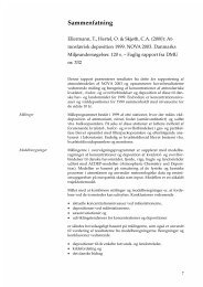
400DEHPConcentration, ng/g d.m.3002001000Depth, cm0 5 10 15 20 25Age, y TwentyForty Sixty EightyFigure 20DEHP in the core of fjord sediment near the WWTP outlet.In Figure 20 a general decreasing tendency of DEHP concentration withdepth can be observed. There is a large scatter of the points, and thereseem to be weak local maxima occurring at depths of 11 and 17 cm. It isevident that old sediment layers contain lesser xenobiotic substance thannewer ones, reflecting a history of increasing pollution.76BBPConcentration, ng/g d.m.543210Depth, 0 cm5 10 15 20 25Age, y TwentyFortySixty EightyFigure 21BBP in sediment coreAs observed in Figure 21, BBP display the same general pattern asDEHP, but with more random variation. More pronounced maxima areseen, occurring roughly at the same depths as for DEHP.44

200NPNPDEConcentration, ng/g d.m.150100500Depth, cm0 5 10 15 20 25Age, yTwentyFortySixty EightyFigure 22NP and NPDE in sediment coreFor NP and NPDE, a very different and interesting pattern is observed inFigure 22, which display two pronounced maxima occurring at depths of7 and 18 cm, respectively. These maxima coincides approximately – butnot precisely - with those observed for DEHP and BBP. A probable explanationfor this observation may be a long-term variation in the consumptionof NPE, since these by an agreement between the detergent industryand the environmental authorities has been phased out in 1989.For the variation with depth, another factor of significance is the new andmore efficient WWTP, taken into operation in 1995. The current efficiencyis described by Fauser et al. (2000).For a more complete understanding of the variation with depth, a modeltaking care of the transport, adsorption and desorption as well as degradationwill be described in section 6.1.4. The model treats only the fateof DEHP, being the most abundant substance.5.3 Streams and lake5.3.1 WaterIn Table 17 the abundances of the substances in the stream and the lakewater are shown as mean and standard deviation of all samples45

Table 17 Abundance of substances in stream and lake water. Mean and standard deviation all samples,ng/lWater, ng/l n Stat NP NPDE DBP DPP BBP DEHP DnOP DnNPHove Å upstream lake G. 4 mean 17 201 0 0.4 2.3 313 4.1 0.5sd 33 402 0 0.8 2.7 218 3.7 1.0Lake Gundsømagle Sø 5 mean 19 230 11 1.6 13 408 20 8sd 43 514 21 2.2 19 428 39 16Hove Å downstream lake G. 4 mean 0 0 0 1.3 4.5 405 108 699sd 0 0 0 1.0 5.4 510 216 1399Maglemose Å near mouth 2 mean 0 0 0 0.2 2.3 158 0.7 0sd 0 0 0 0.1 1.5 139 1.0 0Helligrenden near mouth 4 mean 13 0 0 0.1 1.9 107 1.3 0sd 26 0 0 0.1 1.3 140 2.7 0Total 19 mean 11 103 3 0.8 5.1 298 29 149sd 28 313 11 1.3 9.7 336 100 6410 = not detected.The total means and standard deviations from Table 17 of all stream andlake water samples are shown as bar graphs in Figure 23.700600meanConcentration, ng/l500400300200sd1000NP NPDE DBP DPP BBP DEHP DnOP DnNPFigure 23 Total mean and standard deviations of water in streams and lake.In the water of the streams and the lake, the most abundant phthalateswas DEHP, DnNP and DnOP followed by very low amounts of BBP andDBP as seen from Table 17 and Figure 23. DEHP occurred overall inabout the triple concentrations of those occurring in the fjord. NP occurredin significant concentration, and in contrast to the fjord water, alsoNPDE was found.NPDE was found in Lake Gundsømagle and in Hove Å upstream thelake. These substances thus seem to be removed by sedimentation in thelake, a view supported by the sediment measurements mentioned below.DBP occurred only in the lake and only at low concentrations. Contraryto expectations, an increasing concentration gradient for most phthalates46

was observed in the flow direction in the Hove Å system through thelake. Remarkably, DnOP and DnNP were found at very high concentrationsin Hove Å downstream the lake (near the mouth), indicating a localpollution.The water of the nearby stream Maglemose Å displayed significantlylower concentrations of all substances measured (about the half forDEHP). The water in Helligrenden on the other side of the fjord locatedin a more rural area displayed still lower abundances, approaching thelevel in the fjord water. The spatial and temporal variation of DEHP isshown in Figure 24 and for BBP in Figure 25.The spatial and temporal variations of DEHP and BBP in the water of thestreams as seen from Figs. 24 and 25 were more pronounced and seemedmore random in comparison to the fjord water. This must be expectedsince the streams – unlike the fjord – are hydraulic separate entities locatedin different geographical areas, fed by different sources and havingdifferent flows, which display large variations due to the deposition.12001000DEHP ng/l8006004002000Mar-98Jun-98Sep-98Dec-98Nov-99MeanHove Å ups.Gundsømagle SøÅ Hove downstreamMaglemose Å mouthHelligrenden mouthMeanFigure 24 Spatial and temporal variation of DEHP in water of streams and lake47

5040BBP ng/l3020100Mar-98Jun-98Sep-98Dec-98Nov-99MeanHove Å ups.Gundsømagle SøÅ Hove downstreamMaglemose Å mouthHelligrenden mouthMeanFigure 25 Spatial and temporal variation of BBP in water of streams and lake5.3.2 SedimentIn Table 18 the abundances of the substances in the stream and the lakesediments are shown as mean and standard deviation of all samples. Onlysediment from the Hove Å system was sampled. Within the lake there arethree sampling positions at different distances from the inlet of Hove Å(in the East end of the lake) and near the South bank, respectively.Table 18 Abundance of substances in stream and lake sediment. Mean and standard deviation, allsamples, ng/g dmSediment, ng/g dm n Stat NP NPDE DBP DPP BBP DEHP DnOP DnNPHove Å upstream lake G. 2 mean 32 9 17 0.9 3.8 75 3.6 7.0sd 5 13 23 1.3 0.01 20 0.02 2.3Gundsømagle Sø 100 m W 2 mean 416 341 38 0.4 5.5 93 2.7 5.8sd 19 113 14 0.6 0.5 11 2.1 4.3Gundsømagle Sø 200 m W 2 mean 2362 2278 67 0 2.2 124 1.0 4.2sd 335 425 42 0 0.3 3.7 1.4 1.7Gundsømagle Sø S bank 2 mean 223 0 3 0 1.4 14 1.5 0sd 57 0 2 0 2.0 6.6 2.2 0Hove Å downstream lake G. 6 mean 110 240 3 0.8 1.7 180 2.6 9.2sd 47 251 5 1.5 3.1 115 1.6 6.2Total 14 mean 480 479 19 0.5 2.6 121 2.4 6.4sd 812 797 28 1.1 2.5 94 1.6 5.20 = none detectedThe total means and standard deviations from Table 18 of all sedimentsamples from the streams and the lake are shown as bar graphs in Figure26.48

1000800meanConcentration, ng/g dw600400sd2000NP NPDE DBP DPP BBP DEHP DnOP DnNPFigure 26 Mean and standard deviations of all sediment samples in streams and lake.A prominent feature in Figure 26 is the very high almost equal abundanceof NP and NPDE in the stream and lake sediment, followed byDEHP and much lower concentrations of DBP, DnNP and DnOP.The spatial and temporal variations of DEHP, NP and NPDE in thestream and lake sediment are shown in Figs. 27 to 29, respectively.400DEHP ng/g dw3002001000Jun-98Sep-98Dec-98Nov-99MeanHove Å ups.Lake G. 100 m WLake G. 200 m WLake G. S bankHove Å downstr.Figure 27 Seasonal and spatial variations of DEHP in stream and lake sediment49

400NP ng/g dw3002001000Jun-98Sep-98Dec-98Nov-99MeanHove Å ups.Lake G. 100 m WLake G. 200 m WLake G. S bankHove Å downstr.Figure 28 Seasonal and spatial variations of NP in stream and lake sediment400NPDE ng/g dw3002001000Jun-98Sep-98Dec-98Nov-99MeanHove Å ups.Lake G. 100 m WLake G. 200 m WLake G. S bankHove Å downstr.Figure 29 Seasonal and spatial variations of NPDE in stream and lake sedimentTemporal variationStream gradient50As seen from Figs. 27 - 29, there is a significant temporal variation of theconcentrations in Hove Å downstream the lake Gundsømagle Sø, whichis the only complete seasonal series. Such a variation was also observedfor the water. The variation of the concentration in the sediment at thatposition must be due to a large exchange of substances between waterand sediment due to the high flow velocity, causing suspension of thesediment by turbulence.The mean, shown in the front right row of Figs 27-29, is an expression ofthe spatial variation. This spatial variation in sediment is further illustratedin Figure 30, showing the mean and standard deviation of NP,

NPDE and DEHP in the Hove Å system as bar graphs for the samplingpositions in the flow direction (East to West).30002500NP NPDE DEHPConcentration, ng/g dm200015001000Flow5000Hove Åupstr.Lake G.100 m WLake G.200 m WLake G.S bankHove Ådowns.Figure 30 Mean and standard deviation of most abundant substances in sedimentalong the flow direction of Hove Å system.As noted from Figure 30, DEHP follows a monotonously increasing tendencyin the flow direction, with the exception of the South bank, inwhich very low amounts of all substances occur. This is probably due tothe sandy character of the bottom at that position, in contrast to the organiccharacter at the two other lake positions. The difference may bedue to the action of waves near the bank. Furthermore, assuming themain input to the lake is through Hove Å, the main sedimentation shouldoccur in the line connecting the inlet and outlet in the lake, which is adistance to the North of the South bank. Remarkably, the tendency forNP and NPDE is strongly increasing until the 200 m position in the lake,followed by much lower amounts downstream. The same tendency isseen for DBP and BBP in Table 18.The same trend for these substances was found in the water. An interpretationof these observations would be that the main sedimentationprocess of all substances occurs at the 200m position in the lake, wherethe lake is broad and deepest and the water velocity low. Hence, the substancesare depleted downstream the lake, occurring in considerablylower concentrations in water as well as sediment. DEHP, however, deviatesfrom this pattern, since larger amounts are found downstream.Probably new sources downstream the lake are present.5.3.3 Correlation analysis of streams and lakeIn Table 19 the significant correlations between substances in all lakeand stream water samples are shown (N=19, r crit. = 0.53, p < 0.01). Itappears that the higher phthalates from BBP and up are correlated withDEHP. The same correlations are found in the fjord water, but for that51

matrix, some more correlations were found. This is hardly surprising,given the more diverse character of the different streams, which - unlikethe fjord – are hydraulic separate entities.Table 19 Significant substance correlations in water of streams andlaker BBP DnOP DnNPDEHP 0.65 0.71 0.61p

µg/m²/y000800600400200013-Nov27-Nov12-Dec08-Jan05-Feb05-Mar1996 199702-Apr30-Apr28-May25-Jun09-Jul20-Aug10-Oct24-Oct07-NovDBPDEHPDnOPBBPFigure 31 Deposition of most abundant substances at Lille Valby meteorologicalstation.As observed from Figure 31, for DEHP a minimum occurred in Februaryand a maximum in July. For DBP the minimum and maximum seem tooccur later. This variation reflects the air concentration, which probablyprimarily is driven by the evaporation depending on the temperature.However, also the use of the substances may be of importance.As discussed by Vikelsøe et al. (1999), wind speed and direction seemedto be of lesser significance for the phthalate deposition. This indicatedthat point sources and other local differences played a minor role, longrange transport being more important. Hence, the deposition is approximatelydistributed evenly over the fjord. Further, the specific depositionof the phthalate per area unit g/km 2 /y seemed to be rather independent ofthe wet deposition (rainfall).The mean wind speed and direction is shown for the 1 year sampling periodin the rosette diagram Figure 32.53

Mean wind speed,m/s2 0315 45 N1270090225135180Figure 32 Wind rosette diagram for period of deposition sampling.The wind is primarily blowing from the West across Roskilde Bredning.The single sampling station is therefore believed to represent the depositionof nonylphenols and phthalates in the Bredning with good approximation.54

6 Mathematical data interpretationIn this section the experimental data is interpreted through model simulations.The experimental results show that only DEHP occur in a concentrationthat is of environmental significance. Therefore the physicochemicalprocesses determining the fate of xenobiotics in the watersedimentsystem are identified only for DEHP.Numerical models are set up to assess the fate of DEHP in the sedimentand water compartment of the fjord, respectively. The experimentalsediment core measurements are used to calibrate the sediment modeland a theoretical validation is performed with analytical solutions. Asteady-state mass balance for the water compartment, comprising theDEHP fluxes in the fjord system, is validated with the experimental fjordwater concentrations.6.1 Physico-chemical processesThe considered physico-chemical processes that involve the fate ofDEHP in the water and sediment systems respectively are (cf. Figure 33)Atmospheric depositionh(x)52 1• C w P3WWTPdischarge andfreshwaterrunoff•4C s P241C w = Dissolved conc. in waterC s = Dissolved conc. in porewaterP = Degradation producth(x) = Water depth at distance xxFigure 33 Physico-chemical processes in Roskilde Fjord.1. Microbial degradation.2. Adsorption of molecular xenobiotics to suspended particulate matter.3. Sedimentation of particulate matter.4. Vertical transport of molecular substances and particulate matter insediment.5. Mixing of water volume and transport of molecular substances andparticulate matter in water.55

6.1.1 Microbial degradationThe substance can occur in different phases: As free dissolved molecules,as micelles or microdroplets, as adsorbed to dissolved organic matter(DOM) or adsorbed to fixed organic matter. Only the free dissolvedcompound is accessible for microbial degradation. The phthalates primarilyoccur as micelles due to low solubility and high hydrophobicityand hence only a small fraction of the total substance is biodegradable.The bio-degradation rate is based on the Monod-expression (e.g.Schnoor, 1996) and can be expressed through 1 st order reaction kineticsdCdt=where-⎡ mg ⎤k1 ⋅ C ⎢ ⎥(1)⎣liter⋅sec.⎦k 1 is the pseudo 1 st order degradation rate [sec -1 ].C is the dissolved free molecular concentration of the substance [mg ⋅ litre-1 ].The 1 st order kinetic holds under the following conditions• The concentration of the dissolved degradable substance is muchsmaller than the half saturation constant.• The biomass specific to the actual substance is assumed to be active atall times and the concentration is constantly low in time and homogeneousin the different compartments.• The yield coefficient of the micro-organisms is constant regardless ofthe biomass and substance concentrations. This approximation is veryrough and is only true within narrow concentration limits (Mikkelsen,1994).Different reaction rates can be employed for the degradation of DEHP inthe Fjord water and sediment respectively. In the water phase the concentrationof active biomass is very small and as a rough estimate a reactionrate equal to a factor of 1000 (Furtmann, 1996) lower than the aerobicrate found in the WWTP, k 1N = 10 sec (Fauser et al. 2000) is ex--5 -1pected.In the aerobic sediment surface layer about the same degradation rate asin the WWTP is expected. This layer originates from oxygen diffusionfrom the water to the sediment and/or from mixing through bioturbationof benthic macro-fauna under favourable conditions. The thickness of thelayer can be varying, mainly due to wind conditions and a probable meanvalue will be around 5 cm.Below this layer anoxic (nitrate or sulphate reducing) conditions prevailand a degradation rate of 10% of the aerobic rate is anticipated.56

6.1.2 Sorption and solvationIn the model set-up it is assumed that the adsorption-desorption processesare instantaneous, reversible and linear in concentrations. Comparedto other processes in the system the sorption reactions reachchemical equilibrium quickly and the kinetic relationships related to adsorptioncan therefore be assumed to be steady-state. The reversibility istrue in some cases, but for the phthalates the adsorption is very strongand it is questionable whether the desorption is of any importance. 1 st orderirreversible adsorption has been shown to describe soil adsorptionmore satisfactorily (Sørensen, 1999).Different regimes for simulating adsorption capacities can be employed.The Langmuir adsorption model is defined by a maximum adsorption capacitythat is related to a monolayer coverage of surface sites, which isrepresentative of a wide range of equilibrium sorption isotherms for organicadsorbates in natural waters (Schnoor, 1996).When the number of available sites is large compared to the number ofoccupied sites there is usually a linear relationship between the concentrationof dissolved substance, C (mg ⋅ litre -1 ), and the concentration ofadsorbed substance, C X (mg ⋅ litre -1 ). For a specific adsorbate the concentrationof available sites can be expressed through the particulate drymatter concentration, C XB (kg DM litre -1 ). The adsorption constant specificfor this adsorbate, is expressed through the constant K d .⎡ mg ⎤CX= Kd ⋅ C ⋅ CX B ⎢ ⎥(2)⎣litre⎦K d [litre ⋅ (kg DM) -1 ] is a measure of the actual partition in natural watersthat can be empirically derived from the fraction of organic carbon presentin the particulate matter, f oc , and the organic carbon/water partitioncoefficient for the compound, K oc . This is valid when the organic carboncontent is larger than 0.05 - 0.1 % in environmental matrices. When theorganic content is lower there is an increasing tendency for adsorption tothe inorganic parts of the matrix. This phenomenon is more pronouncedfor polar organic substances.The K d value is characteristic for specific adsorbates. It is assumed thatthere exist different “species” of particulate matter in the system, i.e. atthe WWTP outlet and in the water phase of the Fjord the organic fractionof the particulate matter is relatively high and in the sediment it is lowerdue to degradation. This implies a lower K d value in the sediment. However,K d is defined under steady-state conditions and since it is questionablewhether the retention time in the water is long enough for steadystateto occur, a reduction of K d is appropriate here. On the other hand,the substance entering the Fjord through discharge and deposition will alreadybe adsorbed to DOM and therefore it is more a problem of desorptionin the diluted Fjord water.At the sediment surface the organic fraction will be higher than in thedeeper layers. The sediment density is, however, assumed to be constantthroughout the depth although there will be an increase caused by pressurebuild-up. The former will result in a decreasing retention factor andthe latter in an increasing retention factor for increasing depths.57

Microbial degradation of organic matter can release adsorbed substance.Digestion of organic matter by benthic organisms will remove adsorbedsubstance and degrade or incorporate it in the tissue. The substance willthen be released as adsorbed substance when the organism dies. Theformer process will result in a decreasing K d value and the latter an increasingK d value.As a consequence of these complex interactions only one K d value is assignedto the total system. In the WWTP a K d value for DEHP was foundto be approximately 13000 litre ⋅ kgDM -1 (Fauser et al., 2000). In thiswork K d is set to 10000 due to the lower organic fraction in the particulatematter.For substances that are only sparingly soluble, such as the phthalates, it isnecessary to consider the solubility properties in relation to micelle formationthat removes the compound from its molecular unimeric dissolvedstate to a state of non-degradability. Due to the hydrophobicity ofthe phthalates the dissolved state generally comprises micelles (or microdroplets)even at very low concentrations (Thomsen et al., 2000). Thepresence of detergents will, however, increase the apparent solubility bymicelle formation. With densities close to that of water these micelleswill not form a bulk phase but rather form a colloidal suspension in theaqueous phase.Based on the definition of the dissolved fraction, the regimes in Table 22can be set up.Table 22 Influence of definition of dissolved fraction on the degradationand diffusion processes.“Dissolved” fraction Degradation DiffusionFree moleculesMicellesOverestimatedOverestimatedAdsorbed to DOMFree moleculesOverestimatedRealisticMicellesFree molecules Realistic UnderestimatedThe experimentally found concentrations in the water and sediment aretotal concentrations. A differentiation in dissolved and adsorbed fractionsin the model is based on the K d value found in Fauser et al. (2000) wherethe samples are centrifuged yielding a settled fraction comprising substanceadsorbed to large and small particles (DOM) and a dissolved fractioncomprising free molecules and micelles. In the model calculationsthis will result in an overestimation of the degradation and a realistic estimationof the diffusion in the sediment, cf. Table 22.586.1.3 SedimentationSedimentation is a transport mechanism where particles are brought tothe sediment surface by gravitational settling. Due to turbulence resuspensionof surface layer particles will occur. The resuspended particlesare assumed to comprise the same concentration of adsorbed substanceas the particles in the water phase. It is therefore sufficient to considerthe net sedimentation.

Different standard methods can be used to define the vertical transport ofmatter through the water phase. The sedimentary fraction can be foundfrom standing in e.g. 2 hours (DS/R 233 1973) and the suspended fractionfrom filtering (DS/R 233 1973). The remaining amount is either dissolved(molecular) or colloid. No standardised methods exist that canidentify the transition between these last two groups.The total sedimentary fraction is obtained through centrifugation wherethe sedimentary fraction, suspended fraction and some of the colloidalmatter is comprised. If the particulate matter is defined as particles withdiameters larger than 1 µm the following materials are the predominantcontributors in the sedimentation process.Table 23 Properties for suspended particulate matter (Harremoës etal., 1990).Diameter[µm]Density[g ⋅ cm -3 ]Inorganic: Clay particles 1 - 2 2.5 - 2.7Silt, fine 2 - 6 2.5 - 2.7Silt, medium 6 - 20 2.5 - 2.7Silt, coarse 20 - 60 2.5 - 2.7Organic: Algae 1 - approx. 50 1.01 - 1.03The sedimentation process can be described by a pseudo 1 st order removalof particulate matter from the water phase. Thus, the removal ofadsorbed xenobiotics isdCdtw⋅ Xw⋅ Kdw=- k1sed⋅Cw⋅Xw⋅Kdw⎡⎢⎣mglitre⎤⋅ sec. ⎥⎦(3)wherek1sedv=hsedm1≈hour3 m= 0.331hours= 81daysis the sedimentation constant and v sed is the sedimentation velocity suggestedby Harremoës et al., (1990), h is the water depth. X w is the concentrationof particulate matter in the water. In the following a sedimentationconstant fitted for the present data is found.Extraction is a process whereby the non-sedimentary organic matter canbe transported to the sediment. It comprises adsorption of colloids to thesediment and absorption of molecular substances in micro-organismspresent in the sediment. The resulting concentration gradient across theboundary layer is followed by a vertical diffusive transport from the totallymixed water to the sediment.59

The extraction process can be described by a pseudo 1 st order removal ofdissolved and colloid matter from the water phasedCdtw⋅ θ=- k1ext⋅Cw⋅θ⎡ mg ⎤⎢ ⎥⎣litre⋅ sec. ⎦(4)wherek1extv=hext0.5 - 23 mmday= 0.17 - 0.671daysis the extraction constant and v ext is the extraction velocity (Harremoës etal., 1990).The overall vertical transport can be expressed asdCdtw⋅( θ + X ⋅ K ) = - C ⋅ ( k ⋅θ+ k ⋅ X ⋅ K ) ⇒wdww1ext1sedwdwdCdtw⋅ ( θ + X ⋅ K )=wdwmg⎢⎣liter⋅sec.⎡ ⎤( θ + X ⋅ K ) = - C ⋅ k ⋅ R⎥ ⎦- C w ⋅ k1vert⋅w dww 1vert wThe retention factor R w will be close to unity, i.e. low particulate concentrationsprevail in the water, and therefore k 1vert is approximatelyequal to k 1ext .The extraction process is defined for organic matter that is present inabundant concentrations in the water compartment such as proteins, sugarsand other easily degradable and hydrophilic compounds. For thesecompounds the predominant removal mechanism in the sediment is 1 storder microbial degradation and accordingly this can be related to a 1 storder transfer from the water to the sediment (cf. Equation 4).In this work xenobiotics that appear in very low concentrations and thatare practically insoluble are investigated. The degradation rates are lowand the governing removal/transport mechanism in the sediment is diffusion,which in turn is related to a similar removal rate from the waterphase. The approach is therefore to define the vertical transport of nonsedimentarysubstance in terms of a “suction” caused by molecular concentration-gradientconditioned diffusion in the sediment (cf. Equation19).The transport of sedimentary adsorbed substance can be derived fromEquation 3, where the sedimentation of particles isdXdtw=- k1sed⋅Xw⎡ mg ⎤⎢ ⎥⎣liter⋅ sec. ⎦(5)60

Introducing the concentration of sedimentary particulate matter X w = 10 ⋅10 -6 kg dm ⋅ litre -1 (Larsen, 1999) and an adjusted sedimentation constant,k 1sed = 0.36 days -1 , the sedimentation rate becomesdXdtw=- 0.363651year1010-6kg dm.= -13.2litre10-4kg dmlitre yearThe 23 cm sediment core taken at a position 130 meters from the shoreand WWTP outlet is divided into 0.5 cm sections. It shows a mean watercontent of θ = 0.55 ± 0.13 litre water ⋅ (litre total) -1 and a mean dry mattercontent of X s = 1.06 ± 0.26 kg dm ⋅ (litre total) -1 yielding a solids densityof 1.06 / 0.45 = 2.35 kg dm ⋅ (litre dm) -1 .The sedimentation interacts with resuspension and assuming a net sedimentationrate of 13.2 ⋅ 10 -4 kg dm ⋅ (litre ⋅ year) -1 the annual net accumulationrate, S, at the sediment surface amounts to13.2S =kg dm-410litre yearkg dm1.58litre30 dmmm= 2.5year(6)Where the water depth is 3 m and the dry matter content at the surface is1.58 kg org. dm ⋅ litre -1 . Madsen et al. (1979) found linear accumulationrates in the inner Fjord in the interval 1.2 - 5.8 mm ⋅ year -1 . The historicalsubstance load and hence the substance accumulation rate can be derivedfrom the particle accumulation rate and the substance concentration inthe sediment. However, this is beyond the scope of this report.The total downward transport of substance is thus found from a combinationof diffusive concentration gradient conditioned transport andsedimentation of adsorbed particulate substance.6.1.4 Vertical transport in the sedimentOnce the substances have reached the sediment the dissolved fraction canbe transported further vertically and horizontally. The flux in the sedimentis governed by molecular diffusion. Advection and convection arenegligible processes that are primarily relevant in connection with hydraulicgradients in groundwater studies. Diffusion is not only relevantfor dissolved substances but it has been suggested that also substance adsorbedto dissolved organic matter (DOM) is susceptible to macro moleculardiffusion. This will probably have diffusion coefficients that areconsiderably smaller than the free molecules. According to the previousdefinition only the free molecules and micelles are comprised in the dissolvedfraction in the experimental measurements and adsorption toDOM will therefore not be dealt with here.61

The diffusivity of a molecule depends on the random movements(Brownian motion) which again is dependant on the kinetic (or internal)energy. The kinetic energy is defined as ½ ⋅ m ⋅ v 2 stating that largermolecules have lower mean velocities than smaller molecules, givenequal energy levels. Furthermore the increased cross sectional areas reducethe mean free path in the carrier medium resulting in a lower mobilityof larger molecules compared to smaller molecules.This relationship between molecular size and diffusivity can be used topredict diffusivities of compounds from known diffusivities of othercompounds based alone on the molecular masses, cf. Equation 7(Schwarzenbach et al., 1993)DDunknownknownmassknown≈ (7)massunknownThis requires that the carrier media are the same and that the chemicalstructures are related. Benzene can be used as a model compound forcalculating the diffusivity of DEHP that also contain a benzene ring inaddition to the alkyl chains and ester groups. Schwarzenbach et al.(1993) have found a diffusion coefficient in water for benzene (M w = 78g ⋅ mol -1 ) of approximately 10 -9 m 2 ⋅ sec -1 .DDEHP= Dbenzene⋅mmbenzeneDEHP=1 ⋅ 10-92msec.⋅78391= 5 ⋅ 10-102msec.Fick’s 1st law can describe the vertical substance flux in the sedimentdCS⎡ mg ⎤sz= θ ⋅ Ddisp,sz ⋅dz ⎢⎣m⋅ sec. ⎥(8)⎦N2where θ is the porosity of the sediment and D disp,sz is the dispersion coefficient,defined as2⎡ m ⎤Ddisp, sz= α ⋅ vp+ Dsz⎢ ⎥(9)⎣sec.⎦where α is the longitudinal dispersivity, v p is the advective pore watervelocity (≈ 0) and D sz is the molecular diffusion coefficient.Schwarzenbach (1993) suggests the following empirical relationshipD=D=5100.55=2102msec.1.5-101.5-10(10)disp, szszAdditionally, under favourable conditions, the redistribution of sedimentparticles by benthic macro fauna can occur by a variety of processes.This bioturbation can influence the transport and fate of hydrophobic xenobioticsin the surface layer. The particle reworking and the pumping ofpore water can create a mixed layer where the adsorbed and dissolved62

substances migrate more rapidly than can be accounted for by moleculardiffusion.The extension of the mixing layer is dependent on the macro organism.For lugworm Arenicola marina, which is the predominant benthic organismin the inner Fjord, a 5 to 10 cm bioturbation zone in depths of approximately15 cm can be expected. However, the sediment core wasextremely hard and therefore it is expected that the influence from bioturbationis negligible. This is confirmed by the DEHP concentrationprofile in the sediment core.Thus neglecting the influence from bioturbation, the horizontal concentrationgradient is much smaller than the vertical concentration gradientand the horizontal diffusion can be omitted in the mass balance for amodel sediment volume.6.1.5 Horizontal transport in the waterThe hydraulic effect from the sea will cause a high flow through the narrowparts in the middle of the Fjord. This combination of saline intrusionsand fresh water discharges causes a salinity gradient ranging from20 ‰ in the northern entrance to 14.5 ‰ in the inner parts of the Fjord(Harremoës et al., 1990).In the preceding section it is assumed that the convective flow in thesediment is zero. This excludes the influence of percolation of groundwaterthrough the sediment into the Fjord. This is an assumption that willnot hold at local spots where freshwater intrusions will enter the salineFjord and lower the salinity on a local scale. The approach in this work isto consider net deposition, streams and anthropogenic outlets as the onlyfreshwater sources to the fjord.Due to an effective large scale mixing of the water volumes, which enhancesthe vertical transport of dissolved and particulate matter, the verticalconcentration gradient is negligible, resulting in a mean depth integratedconcentration in the water column. The large scale mixing, whichis caused by a combination of turbulence and convection, is also the predominantprocess in the horizontal transport of water and substances inthe shallow Fjord.The salinity mixing data can be used to calculate an effective longitudinaldispersion coefficient for the narrow part of the Fjord. Assuming auniformly distributed freshwater supply along the shore of 1.16 ⋅ 10 -4 m 3 ⋅(m ⋅ sec) -1 , a mean cross sectional area of 2610 m 2 , a length of 28 km andsalinities of 20 ‰ in the northern entrance and 14.5 ‰ in the Bredning,the effective dispersion coefficient can be calculated from the salinitygradient (Harremoës et al., 1990)Dwx=-4 m1.16 ⋅ 10 ⋅sec.22 ⋅ 2610 m ⋅2( 28000 m)20.0ln14.52=542msec.(11)63

The longitudinal salinity gradient is only constant in the narrow part ofthe Fjord and therefore the dispersion coefficient is only representative ofthis section. In the inner Fjord the salinity is approximately constant andthe horizontal transport is based on other criteria, such as turbulence andconvective mixing.In the inner Fjord, i.e. Roskilde Vig and Bredning, where the dischargefrom Bjergmarken WWTP is situated, the horizontal velocity will be minordue to the larger surface areas. Hydraulic effects from wind andfreshwater sources will govern the mixing. Strong western winds are ableto create water level fluctuations up to 170 cm above mean sea level inthe inner Fjord compared to only ± 10 cm resulting from tidal variations.Therefore, it is not relevant to consider the transport in the Vig andBredning in relation to dispersion, but rather to consider them as mixedbasins.6.2 SourcesDifferent sources contribute to the DEHP concentrations in the Fjord (cf.Figure 2).• The wastewater treatment plant (WWTP) effluent is discharged as apoint source to the surface water at the shore in the inner part of RoskildeFjord (Vig). The flow is 492 ± 356 m 3 ⋅ day -1 with a mean concentrationof 0.7 µg DEHP ⋅ m -3 (Fauser et al., 2000).• The point sources to the Bredning and narrow passage of the Fjord,i.e. WWTP discharges from four smaller cities, are estimated to accountfor the same concentration (C WWTP ) and flow rate (Q WWTP ) as theWWTP in the Vig. The total load from the point sources is distributeduniformly along the horizontal axis (cf. Table 24 and Figure 34).• For Roskilde Bredning and the narrow passage contributions fromfreshwater sources from streams and lakes must be included. Thefreshwater runoff is higher per length unit in the Bredning than in thenarrow passage.• Atmospheric deposition is considered to be uniformly distributed withrespect to time and surface area. The dry deposition rate is 230 µgDEHP ⋅ (m 2 ⋅ year) -1 (cf. Table 21).• For a period of 25 years, ending in 1991, all of the sludge produced inearlier WWTP’s in Roskilde was used for amendment on an agriculturalfield adjacent to the WWTP discharge in the shore. Since 1991the produced sludge has been stored in an intermediary deposit closeto the sludge amended area and shore. Leaching from the sludgeamended soil as well as wash out from the sludge deposit, in case ofheavy rainfall, will contribute to the load in to the Fjord (Vikelsøe etal., 1999).64

• In 1969 in connection with work on the Roskilde harbour, the sedimentwas dumped on the site marked ∇ on the map in Figure 2. Thishas since then been a source of leaching to the Fjord water. The loadhas decreased with time and is today estimated to be negligible comparedto the WWTP discharge.• The flux of saline water from the sea to the Fjord is 3 to 4 times largerthan the freshwater flux to the Fjord (Hedal et al, 1999). In Table 24the three water exchange rates are stated.6.3 Model parametersThe following model parameters are required in the models.Calculated and measured state variablesC w : Concentration of dissolved substance in water phase [mg ⋅ litre -1 ].C s : Concentration of dissolved substance in sediment phase [ng ⋅ g -1 ].Measured model inputsX w : Concentration of suspended particulate matter in water phase= 10 ⋅ 10 -6 kg DM ⋅ (litre total) -1X s : Concentration of dry matter in sediment= 1.06 kg DM ⋅ (litre total) -1θ s : Water fraction in sediment= 0.55 litre water ⋅ (litre total) -1Q WWTP :Discharge flow from WWTP= 492 ± 356 m 3 ⋅ hour -1C WWTP : Concentration of dissolved DEHP in WWTP discharge= 0.7 µg DEHP ⋅ litre -1R WWTP : Retention factor for WWTP discharge= 1.05C tot,dep : Atmospheric bulk deposition= 7.29 ⋅ 10 -15 kg DEHP ⋅ (m 2 ⋅ sec) -1C tot,f : Concentration of mean total substance in freshwater from streams= 0.2 µg DEHP ⋅ litre -1Calibration parametersK d :Distribution coefficient between water and organic matter in wateror sediment [litre water ⋅ (kg DM) -1 ].k 1N : Aerobic pseudo 1 st order removal rate [sec -1 ].k 1D : Anaerobic pseudo 1 st order removal rate [sec -1 ].S: Annual sediment accumulation rate [mm ⋅ year -1 ].Estimated model inputsParameters in Table 24.D wx : Horizontal dispersion coefficient in narrow part of Fjord= 54 m 2 ⋅ sec -1D sz : Molecular diffusion coefficient in sediment= 2 ⋅ 10 -10 m 2 ⋅ sec -1The hydraulic and geographical key data for Roskilde Fjord are shown inTable 24.65

Table 24. Data for Roskilde Vig, Bredning and narrow passage.Vig Bredning Narrow passageSurface area A vig =A bred =A narr =4 km 2 48 km 2 73 km 2Length - L bred =(10 km)Mean depth h =3 mDiffuse freshwaterflowPoint sourceflowWater exchangeQ f,vig =0h =3 mQ f,bred =3.60L narr =28 kmh =3 mq f,narr =1.16 ⋅ 10 -4m 3 ⋅ sec -1 m 3 ⋅ (m ⋅ sec) -1Q p,vig =136.7 ⋅ 10 -3m 3 ⋅ sec -1 Q p,bred =36.0 ⋅ 10 -3m 3 ⋅ sec -1 q p,narr =3.60 ⋅ 10 -6m 3 ⋅ (m ⋅ sec) -1Q bred-vig =Q narr-bred = Q sea-narr =m 3 ⋅ sec -1 m 3 ⋅ sec -1 m 3 ⋅ sec -1(0.5⋅Q f-sea )3.4 (2⋅Q f,sea )13.7 (3⋅Q f,sea )20.5The mean residence time for the entire Fjord is approximately 3 months.6.4 Model set-upRoskilde Vig and Bredning are considered to be totally mixed whereasthe transport in the narrow part of the Fjord is more appropriately describedwith dispersion.66

SeaDispersion modelBox-modelsIsefjordL narrA bredh bredA vigh vigQ sea-narrA narrh narrQ narr-bred Q 2BredningQ 3Q bred-vigQ 1Vig5 kmq f,narr , C f,narr+q p,narr , C p,narrQ f,bred , C f,bredQ p,bred , C p,bredQ f,vig = 0Q p,vig , C p,vigGeneral processes(µg ⋅ (m 2 ⋅ sec) -1 ):Atm. dep.: C depSedim.: S ⋅ R s ⋅ C wDegr.: k 1 ⋅ h ⋅ C wQ 1 = Q sea-narr +(q f,narr +q p,narr )⋅L narr +Q f,bred +Q p,bred +Q p,vigQ 2 = Q narr-bred +Q f,bred +Q p,bred +Q p,vigQ 3 = Q bred-vig +Q p,vigFigure 34 Schematic view of Roskilde Fjord. Symbols and notations are explainedin Table 24.Two model scenarios are set-up that in combination will describe the dynamicand steady-state concentrations based on the processes in the waterand sediment of Roskilde Fjord.Water model:Steady-state box-models of Roskilde Vig and Bredningcombined with a dynamic numerical model of thenarrow passage of the Fjord. Experimental results areused to validate the model. The models are designed toaccount for the overall mass balances in the differentregions of the Fjord.Sediment model: Numerical model including diffusion, sedimentationand degradation. Analytical expressions and experimentalresults are used to validate the model.The models are set up based on the following assumptions• Constant discharge flow (Q WWTP ), freshwater flow (Q f ) and deposition(Q dep ).• Constant discharge concentration (C WWTP ), freshwater concentration(C f ) and deposition concentration (C dep ).• Constant water depth (h).67

• Constant concentrations of suspended matter in water and sediment(X w , X s ).• Equilibrium between dissolved and adsorbed substance (K d ).• Water volume is totally mixed along the vertical axis.• Only vertical diffusive flows in sediment (D sz ).• Dissolved concentration in sediment surface layer is equal to the dissolvedwater concentration.• 1 st order degradation of dissolved substance in water and sediment(k 1 ).• Increasing sediment depth in time due to sedimentation (S).6.4.1 Steady-state box-modelThe values in Table 24 and the model parameters are inserted in the generalsteady-state Equation 12.0 = Point sources + Freshwater sources +Water exchange +Atmospheric deposition + Sedimentation + Degradation ⇒ (12)For Roskilde Vig the mass balance becomes0 = CWWTP⋅ R WWTP ⋅ Q WWTP + C tot,f ⋅ Qf,vig( Q + Q Q ) +C w, vig ⋅ R w ⋅ bred-vig p,vig +Ctot, depvigw,vigvigf, vig⋅ A - C ⋅ S ⋅ A ⋅ R - k ⋅ C ⋅ A ⋅ h (13)sThe equations for Roskilde Bredning and narrow passage are describedanalogously. In the Vig equation C w,bred is unknown. In the Bredningequation C w,vig and C w,narr (boundary) are unknown and in the equation forthe narrow passage C w,bred is unknown. Through iteration in the watermodel the unknowns are determined.The calculated contributions and mean water concentrations are summarisedin Table 25.1-w,vigvigvig6.4.2 Numerical models (water and sediment model)The mass balance for the water compartment of the Vig and Bredning areas shown in Equation 13. The water balance in the narrow passage is describedwith the expressions below. Transport in the sediment is describedbelow irrespective of the model for the water.In Figure 35 a vertical section of the water-sediment system is shown.The considered horizontal and vertical mass fluxes are stated for eachcompartment.68

AtmosphericdepositionxdxN wx + ∂ N wx ⋅ dx∂ xC w (x)N wxhN szzC s (x,z)•dzN sz + ∂ Nsz ⋅ dz∂ zFigure 35 Vertical sectional view of the water-sediment system in the narrow passageof Roskilde Fjord.The time incremental mass balance for a water volume dx ⋅ b ⋅ h and asediment volume dx ⋅ b ⋅ dz isdC A ⋅ R ⋅ dx ⋅ b ⋅ dz =dt⎛N b dz - N + dN x ⎞x ⋅ ⋅ ⎜ x ⋅ dx ⎟ ⋅ b ⋅ dz +⎝ dx ⎠⎛N dx b - N + dN z ⎞z ⋅ ⋅ ⎜ z ⋅ dz ⎟ ⋅ dx ⋅ b +⎝ dz ⎠∑k 1i ⋅ C A ⋅ dx ⋅ b ⋅ dz ⇒ (14)dCdt= - dN dx1R - dN 1dz R - k⋅ ⋅ ∑ ⋅ C A(15)RA x z 1where N x and N z are the mass fluxes [g ⋅ (m 2 ⋅ sec) -1 ] along the x and zaxis respectively of substance A with dissolved concentration C A . k 1 is apseudo 1 st order process constant. Equation 15 is the result of twodimensionalmodelling assumptions and can be formulated for the waterand sediment compartment respectively.Water (narrow passage):The horizontal flux is a result of advection and dispersionQ∂ Cnarrw,narrNwx= ⋅ Cw,narr ⋅ Rw- Dwx ⋅ ⋅ Rwb ⋅ h∂ x(16)where (cf. Figure 34)Q narr = Q f,bred + Q p,bred + Q p,vig + (q f,narr + q p,narr ) ⋅ x69

The vertical flux is a combination of sedimentation of particles, extractionof molecular substance through sediment suction, atmosphericdeposition and freshwater sources.∂ CsN wz = - D sz ⋅ - S ⋅ R ⋅ C + C∂ zz=0q f,narrq p,narr+ ⋅ C tot,f + ⋅ Cbbs w,narr tot,deptot,p (17)The first term in Equation 17 is the boundary condition at the sedimentsurface caused by sediment “suction” of substance. The total mass balancefor the water compartment furthermore includes 1 st order degradationand thus becomes( q + q )∂ Cw,narr ∂= Q Cnarr w,narr f,narr p,narr⋅ +⋅ C w,narr +∂ t b ⋅ h ∂ xb ⋅ h2∂ Cw,narrDsz∂ CsD wx ⋅ - ⋅ +2∂ x R w ⋅ h ∂ zz=0CdepR h - S ⋅ R s⋅ C w,narr- k 1⋅ Cw,narrw ⋅ R w ⋅ h R wq f,narrq p,narr⋅ C tot,f +⋅ Ctot,p(18)b ⋅ h ⋅ Rb ⋅ h ⋅ RwBoundary conditions:C w,narr = C w,bred for x = 0C w,narr = C w,sea = 0 for x = L narr + 5 kmwSediment:The horizontal flux is negligible. The vertical flux arises from moleculardiffusion and advection from sediment build-upN = - Dszsz∂ Cs⋅ + S ⋅ R s ⋅ C∂ zw(19)The total mass balance for the sediment compartment is∂ C∂ ts= D Rszs2∂ Cs∂ Cs - S - k 1⋅ ⋅ ⋅ C2s(20)∂ z ∂ z RsIn the upper 5 cm the aerobic degradation rate, k 1N , is used and furtherdown the anoxic degradation rate, k 1D , is used.The two coupled 2 nd order differential Equations 18 and 20 each havingtwo independent variables, x and t for the water model and z and t for thesediment model respectively, can be solved numerically using a grid consistingof discrete nodes for the (x,t) and the (z,t) system respectively,and by employing a forward time central space scheme (cf. Figure 36).70

tWater gridxo• • •i+1 i i-1x in+1nn-1t nTime derivativeSecond space derivative(dispersion)Second space derivative(diffusion)• Known concentrationo Unknown concentrationt nn+1 n n-1j-1•oj• z jj+1•Sediment grid at x itzFigure 36 Time-space grids for the water and sediment models respectively.The numerical interpretation of the sedimentation term S ⋅ R s ⋅ C w is accountedfor by increasing the sediment thickness with an extra layer, dz,each timet = dzsed (21)Sis fulfilled. With a step size of dz = 0.01 m and an accumulation rate of S= 2.5 mm ⋅ year -1 , cf. Equation 6, an additional layer with thickness dzmust be added every 4 years. In doing so the entire concentration profileis moved downward one grid point. The sediment difference equationbelow does therefore not comprise a sedimentation term.71

Water (narrow passage):n+1wn() ()C i = C i+ dt ⋅w⎛⎜ Q narr⎜⎝b ⋅ h⎛+ dt ⋅ ⎜ D⎜⎝- dt ⋅+ dt ⋅+ dt ⋅wx⋅⋅⎛⎜ Dsz⋅⎜⎝R w ⋅ hnn( Cw( i + 1) - Cw( i)) ( q f,narr + qp,narr)dx+b ⋅ hnnn( Cw( i+1 ) - 2 ⋅ Cw() i + Cw( i-1))⎛ Cdep⋅⎜⎝ R ⋅ h - S R sR ⋅ hw⎛ q f,narr⎜⎝ b ⋅ h ⋅ RSediment:n+1nC i,j = C i,js+ dt- dt ⋅dxnn( Cs( i,j+1 ) - Cs( i,j))w⋅wdz⋅C +tot,f2⎞⎟⎟⎠j=0⎞⎟⎟⎠n( ) ⋅ C ( i)C i -kRn 1wwqp,narrb ⋅ h ⋅ R( ) s ( )⎛nnnC ( i,j+1 ) - 2 ⋅ C ( i,j ) + C ( i,j-1)Dsz⋅ ⎜⎜⎝ R s⎛ k⎜⎝ R1s⋅⋅ C( sss )ns( i,j)dz2w⋅Cw⎞⎟⎠⎞⎟⎠⋅Cnw⎞⎟⎟⎠( i)tot,p (22)⎞⎟ (23)⎠For j = 0 the second space derivative in Equation 23 is⎞⎟⎟⎠nnn( Cs( i,1 ) - 2 ⋅ Cs( i,0 ) + Cs( i,0))dz2(24)At time step n: The input sediment surface concentration C s (i,0) to thesediment equation, is calculated from the water equation at the same timestep, because of the faster dispersion in the water phase compared to thediffusion in the sediment.At time step n + 1: The input sediment surface concentration C s (i,0) tothe water equation is calculated from the sediment equation at time stepn.The models are validated with analytical solutions. The experimental andanalytical concentration profiles will be aggregated and discussed in sections6.5 and 6.6 for the sediment and the water compartments respectively.72

6.4.3 Dynamic solution to the diffusion and sedimentation problemin the sedimentThe combined dynamic diffusion, sedimentation and degradation problemis complex to solve analytically. The determination of the concentrationprofile in the sediment at any given position in the Fjord, istherefore simplified to a problem of diffusion and sedimentation in asemi-infinite medium, where the boundary (water) is kept at a constantconcentration. It is acceptable to consider the water concentration as constantin time due to the high horizontal dispersion and vertical mixingthat prevail in the water phase compared to the slower sedimentation toand diffusion in the sediment.The boundary condition is thusC s (x,0) = C w (x) steady-state for t > 0Initial conditionC s (x,z) = 0 for t = 0The solution of the one-dimensional diffusion and sedimentation equation,i.e.∂ C∂ ts= D Rszs2∂ Cs∂ Cs⋅ - S ⋅ (25)2∂ z ∂ zwith the initial and boundary conditions stated above, is (Sørensen et al.,2000)C = 0.5s⋅Cw⎛ ⎛ R s ⎛ z ⎞⎞⎞⎜erfc⎜0.5⋅ ⋅ ⎜ - S ⋅ t ⎟⎟+ ⎟⎜ ⎝ Ds⎝ t ⎠⎠⎟⋅ ⎜⎟ (26)S ⋅ Rs⎜⎛DR s ⎛ z ⎞⎞⎟s⎜e ⋅ erfc⎜0.5 ⋅ ⋅ ⎜ + S ⋅ t⎟⎟⎟⎝⎝ Ds⎝ t ⎠⎠⎠where erfc ( ) is the complementary error function.6.4.4 Steady-state solution to the diffusion, sedimentation anddegradation problem in the sedimentUnder steady-state conditions the following linear homogeneous secondorder equation is valid in the sediment compartmentDR2szSdC2dzS2dCSdCS - S - k 1⋅ ⋅ ⋅ C = 02S ⇔dz dz R- S ⋅ RDszSSdCS k1⋅ - ⋅ C S = 0(27)dz Dsz73

It can be solved according to Spiegel (1968) with the boundary conditionsC s → 0 for z → ∞C s = C w (steady-state) for z = 0And the solution becomesC ( z) = C ( steady −state) ⋅ esw⎛2 ⎞⎜ S ⋅ RsD 2 - ⎛ S ⋅ Rs⎞ k1+⎟⎜ ⎟z⎜ sz ⋅ ⎝ D sz ⋅ 2⎠Dsz ⎟ ⋅⎝⎠(28)6.5 Discussion of experimental and analytical results inthe sedimentIn Figure 37 the numerical model is validated with the analytical solutionto the diffusion and sedimentation problem, cf. Equation 26. The degradationis set to zero in the numerical model. The input values are characteristicfor DEHP and are as stated in the discussion of Figure 38.The simulated time is 50 years and the optimum time step, with respectto run time and precision, is dt = 10 5 sec. The vertical step size is dz = 1cm.350Total concentration in sediment[ng DEHP / gD.W.]3002502001501005000 0,05 0,1 0,15 0,2 0,25 0,3Depth in sediment [m]Dynamic(diff+sed)Dynamic(diff)Numerical(diff+sed)Numerical(diff)Figure 37 Validation of numerical sediment model (Equation 23) with analyticalsolution (Equation 26).Two cases are considered; diffusion combined with sedimentation anddiffusion alone. For diffusion combined with sedimentation the analyticalcurve is only calculated to a depth of 20 cm due to mathematical instabilitiesat larger depths. The sedimentation process in the numericalmodel, where discrete layers of thickness 1 cm are added, is seen to besatisfactorily described compared to the analytical solution. A situationof sedimentation alone will produce a horizontal curve through 300 ngDEHP ⋅ g DM, that will extend to a depth of S ⋅ 50 years ≈ 12 cm.74

The two diffusion curves and the two diffusion + sedimentation curvesare coincident, which implies that the numerical sediment model is consideredto be properly validated.In Figure 38 the validated numerical model is calibrated with the experimentalsediment concentration profile sampled 130 m from theWWTP discharge, cf. section 5.2.3.The model simulations uses the following parametersS = 2.5 mm ⋅ year -1k 1N = 2 ⋅ 10 -5 sec -1k 1D = 8 ⋅ 10 -6 sec -1 (below a depth of 5cm)K d = 10000 litre water ⋅ (kg dm) -1Total concentration in sediment[ng DEHP/g D.W.]350300250200150100500ExperimentalNumerical model(diff+sed+degr)Steady-State(diff+sed+degr)0 0,05 0,1 0,15 0,2 0,25Depth in sediment [m]Figure 38 Experimental sediment core concentrations at distance 130 from discharge,numerical sediment model (Equation 23) and steady-state solution(Equation 28).The curve in the upper 5 cm decreases according to the typical transportdegradationsituation with a constant degradation rate. The high degradationrate indicates aerobic conditions. This rate is the same order ofmagnitude as the aerobic rate found in the WWTP although the biomassand oxygen concentrations are considerably lower in the sediment.Deeper down in the sediment the profile flattens out and decreases withonly 10 % in 5 cm. The oxygen concentration is probably negligible. Adegradation rate of 8 ⋅ 10 -6 sec -1 points to either anoxic or anaerobic conditions.The periodic fluctuations from 12 to 20 cm are probably experimentalnoise but bioturbation by lugworm (Arenicola marina) could produce azone in depths around 10 to 20 cm corresponding to the experimentallyfound. As mentioned previously circumstances that disconfirm this suggestionare the hardness of the sediment core.The interpretation of the experimental data leads to two cases; The fluctuationsbelow approximately 12 cm are noise and the concentrations arezero. This gives a sedimentation rate of 2.5 mm ⋅ year -1 . Alternatively the75

concentration profile below 10 cm is approximately constant down to adepth of minimum 20 cm. In this case the sedimentation is equal to orlarger than 4.5 mm ⋅ year -1 , since diffusion alone can not transport thisamount of substance down to these depths.In the model set-up the sedimentation is described as a discontinuousprocess where a layer of dz = 1 cm is added every 4 years but in realitythe sedimentation occurs in two annual maxima, one in the spring andone in the autumn. The differences in sediment application rate havebeen investigated in the numerical model and the results are identical.The organic concentrations in the sediment and in the particulate materialin the outlet from the WWTP and from atmospheric deposition arelower compared to the biomass in the bio-reactors in the WWTP. The adsorptioncoefficient, K d , is therefore lower than the adsorption coefficientsin the WWTP.The last curve in Figure 38 is the steady-state profile, cf. Equation 28.From observing the profile development for increasing time and fromflux considerations by Sørensen et al. (2000), it can be seen that the timeneeded to achieve steady-state is governed by the accumulation rate.With S = 2.5 mm ⋅ year -1 steady-state is reached in the upper 2.5 cm after10 years. It is only in the immediate theoretical upstart of the process, t =0, that the concentration gradient at the sediment surface will be infinitelyhigh and that diffusion will dominate the flux (Sørensen et al.,2000).This fact can be further substantiated by calculating the flux at the sedimentsurface during steady-state, from differentiating Equation 28 for z =0 and inserting it in Equation 19.k D= C (steady state) S R 0.5 + 0.25 +(29)sz ws1 szN 2( S R )sIn Figure 39 the ratio flux sedimentation ⋅ (flux total ) -1 is plotted for realisticvalues of the products k 1 ⋅ D sz and S ⋅ R s .76

Fluxsedimentation /Fluxtotal1,00,90,80,70,60,50,40,30,20,10,0k1 * Dsz[m2 * sec-2]0,00E+008,00E-141,60E-132,40E-133,20E-134,00E-130,0 20,0 40,0 60,0 80,0 100,0 120,0S * Rs [m * year-1]Figure 39 The importance of sedimentation with respect to the flux of substance tothe sediment.Higher degradation rates yield increasing concentration gradients andthus higher diffusion rates through the sediment. Higher adsorption coefficients,K d , and therefore higher retention factors, R s , result in higher adsorptionto particulate matter, SOM and DOM, and accordingly in highersedimentation rates of adsorbed substance.Therefore hydrophobic substances are transported to the sediment athigher rates than hydrophilic substances.For DEHP the ratios k 1N ⋅ D sz = 2.0 ⋅ 10 -15 m 2 ⋅ sec -2 and S ⋅ R s = 26.5 m ⋅year -1 result in a sedimentation flux comprising about 95 % of the totalflux to the sediment.The sediment concentration profiles of NP and NPDE in Figure 22 differfrom the DEHP profile. The concentrations are approximately zero in theupper 5 cm after which a maximum occurs at a depth of 8 cm. Thequalitative profile can not be simulated analogously to DEHP, where aconstant input concentration in the water is assumed. It is necessary tointroduce a water concentration that varies in time, either as a consequenceof changing emissions or because a new and more efficientWWTP were taken into operation in 1995. The exact emission pattern ofNP and NPDE is not known and therefore it is not relevant, with respectto model calibration, to try to simulate this, in order to achieve the concentrationprofiles in Figure 22.6.6 Discussion of experimental and analytical results inthe water compartmentExperimental measurements in the water compartment at the markedsampling sites, cf. Figure 1 yield a mean DEHP concentration of 91 ± 81ng DEHP ⋅ litre -1 that is approximately constant throughout the fjord.77

To obtain an estimate of the DEHP mass flows in the Fjord system anintegrated mass balance, cf. Equation 12, comprising the two box modelsand the dispersion model is performed in an iterate process. The calculationsassume constant flows and concentrations for the DEHP sources.Steady-state will occur already after a few months in the water compartmentand it is therefore appropriate to consider the steady-state situationalone.For simplicity reasons the diffusive suction by the sediment is omitted,which is in accordance in steady-state considerations. The biomass concentrationin the water is a factor of 100 lower than in the WWTP andfurthermore it is not adapted to optimum DEHP degradation, thereforethe degradation rate per litre is set to be a factor of 1000 lower than in theWWTP, k 1 = 2 ⋅ 10 -8 sec -1 . This is probably still too high but it is compensatedby the removal by volatilisation.Apart from the degradation rate, there are no adjustments of the modelparameters in order to fit the modelled results to the experimental findings.In Table 25 and Figure 40, the steady-state DEHP contributions (+) andremovals (-) to the fjord water compartment, are shown in µg DEHP ⋅sec -1 .Table 25 Mass contributions in µg DEHP ⋅ sec -1 for the Vig, Bredningand narrow passage calculated from the water model.Vig Bredning Narrow passagePoint sources + 100(37 %)FreshwatersourcesNet water exchangeAtmosphericdeposition0(0 %)- 30(11 %)+ 30(11 %)Sedimentation - 100(37 %)Degradation - 10(4 %)+ 30(1 %)+ 720(33 %)- 80(4 %)+350(16 %)- 950(43 %)- 70(3 %)+ 70(3 %)+ 650(26 %)- 250(10 %)+ 530(21 %)- 940(38 %)- 70(3 %)78

µg DEHP / sec10008006004002000-200-400-600VigBredningNarrowpassageDEHP m ass flow inw ater com partm entFreshw ater sourcesPoint sourcesNet w ater exchangeAtm ospheric dep.Sedimentation-800-1000Degradation-1200Figure 40 Mass contributions in µg DEHP ⋅ sec -1 for the Vig, Bredning and narrowpassage calculated from the water model.The calculated total mean steady-state concentrations for the three regionsof the Fjord areVig: 32 ng DEHP ⋅ litre -1Bredning: 26 ng DEHP ⋅ litre -1Narrow passage: 19 ng DEHP ⋅ litre -1 (mean, cf. figure 41)It can be seen that the freshwater sources from streams are the main contributorsto DEHP in the Fjord water followed by atmospheric depositionand WWTP discharges. The removal processes are highly dominated bysedimentation, followed by water exchange with the sea and degradationbalances the contributions.The experimental sediment surface concentrations increase towards theinner parts of the Fjord. In the Vig the DEHP concentration is a factor of2 higher than in the Bredning and a factor of 10 higher than in the narrowpassage. In the narrow passage the flow and turbulence are considerablyhigher and the net sedimentation rate is reduced.By using the calculated steady-state concentration for the Bredning asboundary condition in the numerical solution for the narrow passage, thewater concentration profile in Figure 41 is obtained.79

Total water concentration[ngDEHP / liter]50403020100BredningNarrow passageModelEksperimentel * 0.2Mouth of fjord toIsefjord0 10000 20000 30000Distance from Bredning [m]Figure 41 Total DEHP concentrations in the water in the narrow passage. Numericalmodel (Equation 22) and experimental measurements divided by a factorof 5, cf. Table 9.The experimental concentrations in the water compartment are approximatelyconstant in all sections of the Fjord (5 sampling sites), cf. Figure 4and do therefore not display the characteristic decrease caused by dispersionas seen in Figure 41. The experimental concentration peak around11 km (Frederiksund), arise from an area with very high current and resuspensionof settled material with adsorbed DEHP is a possible explanationto the high water concentration. A reason for the underestimationof the calculated concentrations could be missing contributions fromsources such as boats, spills from industrial activities or leaching fromdumped slag which is reported to have taken place in the Vig.With a mean experimental water concentration of 91 ng DEHP ⋅ litre -1 ,there is a discrepancy by a factor of 3 – 5 compared to the modelled waterconcentrations. This is considered to be acceptable as a model result,but in order to use the model as a risk assessment tool the deviation mustbe taken into account in calculating the predicted environmental concentration(PEC).80

7 ConclusionsDEHP was the most abundant substance found in the fjord water,followed by a much lower concentration of DBP, and minute amounts ofBBP, DPP and NP. NPDE was not detected. The concentrations werevery low, about a third of deposition and half of the small streams.No significant spatial variation of the concentration for any substancewas found in the fjord water on a large geographical scale. A significantseasonal variation was found for DEHP and BBP having maximum inJune and minimum in December. The variation was lesser at the innerpart compared to the middle and the outer part of the fjord. At the narrowmiddle part the seasonal variation was highest, and a significant shorttermvariation was observed having a time-scale of hours.For the streams, the concentrations in the water were about the triple ofthe fjord, the spatial and temporal variations being more pronounced andrandom.In the fjord sediment DEHP and DBP were most abundant, occurring inmuch higher concentrations than in the water. The concentrations decreasedabout 20 times depending on distance from the WWTP outlet. Ina 22 cm deep core of fjord sediment, the DEHP concentrations decreasedabout 10 times from top to bottom.The concentrations found in the fjord water seem too low to adverselyaffect the environment, whereas the substances found in the sedimentsmay influence the bottom living organism, and through them enter thefood chain.The experimental results were used to calibrate numerical models thatwere set up for the water and sediment system respectively. Additionally,analytical solutions were used to perform a theoretical validation. Thegeneric compartment model, SimpleBox, comprised in the EuropeanUnion System for the Evaluation of Substances, EUSES, was evaluatedwith respect to sediment uptake of the hydrophobic compound DEHP.In the water compartment, a mass balance for the annual mean DEHPconcentrations, comprising contributions from wastewater treatmentplants, atmospheric deposition and freshwater contributions and removalsfrom microbial degradation and sedimentation, was performed. It revealedthat the main removal process in the fjord is sedimentation ofparticle bound substances, or binding of dissolved substances to sediments,whereas horizontal transport through the water seems to be oflesser significance. The main contributors are freshwater sources fromstreams followed by atmospheric deposition and discharges from wastewatertreatment plants.The fate of xenobiotics, exemplified with DEHP, in the sediment compartmenthas been described with sedimentation, diffusion and 1 st orderdegradation. However, diffusion will only be significant in the upstart81

phase and can therefore be omitted in model calculations when steadystateconditions are concerned. Such situations typically occur in thesurface layer after about 10 years. As concluded by Sørensen et al.(2000) the insignificance of gradient conditioned diffusion in the surfacelayer, justifies the use of a sediment description comprising a totallymixed sediment compartment, such as the set-up used in the mathematicallymore simple SimpleBox.The used modelling approach, where the water and sediment compartmentsare treated separately only connected through substance exchangethrough sedimentation, seems appropriate in describing the fate of DEHPin the complex multi media fjord system.82

8 ReferencesBerger, W.H. & Heath, G.R. (1968): Vertical Mixing in Pelagic Sediments.Journal of Marine Research, 26, 134 – 143.Carbonell, G, Ramos, C., Pablos, M.V., Ortiz, J.A. & Tarazona, J.V.(2000): A System Dynamic Model for the Assessment of Different ExposureRoutes in Aquatic Ecosystems. The Science of the Total Environment,247, 107 – 118.Fauser, P., Sørensen, P.B., Vikelsøe, J. & Carlsen, L. (2000): Phthalates,Nonylphenols and LAS in Roskilde Wastewater Treatment Plant –Fate Modelling Based on Measured Concentrations in Wastewater andSludge. Ministry of Environment and Energy, National EnvironmentalResearch Institute, Department of Environmental Chemistry, ResearchReport submitted for publication.Fischer, H.B. (1972): Mass Transport Mechanisms in Partially StratifiedEstuaries. Journal of Fluid Mechanic, 53, 671 – 687.Fischer, H.B., Imberger, J., List, E.J., Koh, R.C.Y. & Brooks, N.H.(1979): Mixing in Inland and Coastal Waters. Academic Press.Flindt, M., Madsen, M. & Sørensen, P.S. (1992): Modelsystem forFjorde og Bugter. Havforskning fra Miljøstyrelsen, 9.Flindt, M.R., Kamp-Nielsen, L., Marques, J.C., Pardal, M.A., Bocci,M., Bendoricchio, G., Salomonsen. J., Nielsen, S.N. & Jørgensen, S.E.(1997): Ecological Modelling, 102, 17 – 31.Flindt, M., Pedersen, C.B., Hansen, L.R. & Hedal S. (1998): HydrografiskModellering af Typeområdet Roskilde Fjord 1998. NOVA2003 Årsrapport, Roskilde og Frederiksborg Amter.Furtmann, K. (1996): Phthalates in the Aquatic Environment. Landesamtfür Wasser und Abfall Nordrhein-Westfalen.Harleman, D.R.F. & Thatcher, M.L. (1974): Longitudinal Dispersionand Unsteady Salinity Intrusion in Estuaries. La Houille Blanche, ½, 25 –33.Harremoës, P. & Malmgren-Hansen, A. (1990): Lærebog i Vandforurening.Polyteknisk Forlag.Hedal, S., Hansen, L.R., Thingberg, C. & Jensen, K.B. (1999): Overvågningaf Roskilde Fjord 1998. Roskilde Amt, Teknisk Forvaltning ogFrederiksborg Amt, Teknik og Miljø.83

Holley, E.R., Harleman, D.R.F. & Fischer, H.B. (1970): Dispersion inHomogeneous Estuary Flow. Journal of the Hydraulics Division, Proceedingsof the American Society of Civil Engineers, 1691 – 1709.Larsen M. (1999): Personal communication.Larsen, T. & Hansen, T.B. (1998): Modellering af Næringssalte iFjorde. Vand & Jord, 3, 120 – 123.Madsen, P.P. & Larsen, B. (1979): Bestemmelse af Akkumulationsrateri Marine Sedimentationsområder ved Pb-210 Datering. Vand, 5, 2 - 6.McCall, P.L. & Tevesz, M.J.S. (1982): Animal-Sediment Relations, TheBiogenic Alteration of Sediments. Plenum Press, New York and London.Mikkelsen, J. (1994): Matematisk Modellering af Kemikaliers Skæbne iRenseanlæg. Danmarks Tekniske Højskole, Lyngby, Denmark.Møhlenberg, F. (1995): Regulating Mechenisms of PhytoplanktonGrowth and Biomass in a Shallow Estuary. Ophelia, 42, 239 – 256.Peters, H. (1999): Spatial and Temporal Variability of Turbulent Mixingin an Estuary. Journal of Marine Research, 57, 805 – 845.Pilegaard, K. (1997): Risø National Laboratory. Data collected duringthe RIMI project (Risøs Integrerede Miljøprojekt). Private communication.Remberg, M. (1999): Analysis of phthalate esters in Swedish lakes andrivers. Presented at Phthalate Esters Environmental Analysis Workshop,arr. ECPI, Kortrijk, Belgium, 4-5 Nov. 1999.Roskilde County & Municipality (1994): Hydrografic investigation ofRoskilde Fjord. Reports from Danish Hydraulic Institute and Water Consult.Roskilde County (1999): Rambøll, Hydrometriske beregninger 1998 RoskildeAmtSchnoor, J.L. (1996): Environmental Modelling – Fate and Transport ofPollutants in Water, Air and Soil. Environmental Science and Technology.A Wiley-Interscience series of texts and monographs. John Wiley &Sons, inc.Schwarzenbach, R., Gschwend, P.M. & Imboden, D. (1993): EnvironmentalOrganic Chemistry. John Wiley & Sons, Inc.Shang, D.Y, MacDonald, R.W. & Ikonomou, M.G. (1999): Persistenceof Nonylphenol Ethoxylate Surfactants and Their Primary DegradationProducts in Sediments from near a Municipal Outfall in the Strait ofGeorgia, British Columbia, Canada. Environmental Science and Technology,33, 1366 – 1372.84

Smith, R. (1986): Mixing and Dispersion in Estuaries: Which MathematicalModel and When? International Conference on Water QualityModelling in the Inland Natural Environment, Bournemouth, England:10 – 13 June, 1986, 375 - 385.Spiegel, M.R. (1968): Mathematical Handbook of Formulas and Tables.Schaum’s outline series. McGraw-Hill Book Company.Sørensen, P.B., Fauser, P., Carlsen, L & Vikelsøe, J. (2000): Evaluationof Sub-Process Validity in the TGD in Relation to HydrophobicSubstances. Ministry of Environment and Energy, National EnvironmentalResearch Institute, Department of Environmental Chemistry, ResearchReport submitted for publication.Sørensen, P.B. (1999): Personal communication.Thomsen, M., Carlsen, L. & Hvidt, S. (2000): Solubilities and SurfaceActivities of Phthalates Investigated by Surface Tension Measurements.Environmental Toxicology and Chemistry, in press.Toppari, J., Larsen, J.C., Christiansen, P., Giwercman, A., Grandjean,P., Guilette Jr, L.J., Jégou, B., Jensen, T.K., Jouannet, P., Keiding, N.,Leffers, H., McLachlan, J.A., Meyer, O., Müller, J., Meyts, E.R.-D.,Scheike, T., Sharpe, R., Sumpter, J., & Skakkebæk, N.E. (1995): Malereproductive health and environmental chemicals with estrogenic effects.Miljøstyrelsen, Miljøprojekt nr. 292.van der Velde, E.G., de Korte, G.A.L. Linders, S.H.M.A. & Hijman,W.C (1999): Method development for the analysis of phthalates in environmnetalsamples with GC-MS. Presented at Phthalate Esters EnvironmentalAnalysis Workshop, arr. ECPI, Kortrijk, Belgium, 4-5 Nov. 1999.Vikelsøe, J., Thomsen, M. & Johansen, E. (1998): Sources of phthalatesand nonylphenols in municipal waste water. NERI technical report No.225.Vikelsøe, J., Thomsen, M., Johansen, E. & Carlsen, L. (1999): Phthalatesand Nonylphenols in Soil – A Field Study of Different Soil Profiles.Ministry of Environment and Energy, National Environmental ResearchInstitute, Department of Environmental Chemistry, Technical Report No.268.Wheatcroft, R.A., Jumars, P.A., Smith, C.R. and Nowell., A.R.M.(1990): A Mechanistic View of the Particulate Biodiffusion Coefficient:Step Lengths, Rest Periods and Transport Directions. Journal of MarineResearch, 48, 177 – 207.85

9 AbbreviationsAnalyteBBPDD 4 -BBPD 4 -DBPD 4 -DEHPD 4 -DnOPDBPDEHPDnNPDnOPDPPdm %dmGCGC/MSHRMSLDmg/kg dwµg/kg dwMSndnon-detectDEPANERISubstance analysedButylbenzylphthalateDeuterium ( 2 H, heavy isotope of hydrogen)BBP deuterium-labelled in ringDBP deuterium-labelled in ringDEHP deuterium-labelled in ringDnOP deuterium-labelled in ringDi(n-butyl)phthalateDi(2-ethylhexyl)phthalateDi(n-nonyl)phthalateDi(n-octyl)phthalateDipentylphthalateContent of dry matter in weight percent of totalDry matterGaschromatographyGC combined with MSHigh resolution MS (high ability of MS to discriminatebetween masses)Limit of determination, concentration below which the resultis uncertainMilligram per kg dry weight (Parts Per Million, PPM)Microgram per kg dry weight (Parts Per Billion, PPB)Mass spectrometryNot detected, non-detectResult < 0 after subtraction of the blankDanish Environmental Protection AgencyNational Environmental Research Institute87

NPNPDENPEPAEPFKPhthalatesdSIMSpikeSteady-stateWWTPwwNonylphenolNonylphenol-diethoxylateNonylphenol-ethoxylatesPhthalate esterPerfluoro kerosene (calibration gas for HRMS)Di ester of phthalic acid (1,2-benzene dicarboxylic acid)Standard deviationSelected ion monitoring (MS operating mode)Labelled substance added during the analytical procedurefor quality controlSituation with constant conditionsWastewater treatment plantWet weight88

10 VariablesA bred Surface area of Roskilde bredning (km 2 )A narr Surface area of narrow passage (km 2 )A vig Surface area of Roskilde Vig (km 2 )bCC AC swidth of fjord compartment (m)Dissolved concentration (ng pr. litre)Dissolved concentration of substance A (ng A pr. litre)Dissolved DEHP concentration in sediment pore water(ng pr. g dm)C s (x or i,z or j) Dissolved DEHP concentration in sediment at position (xor i, z or j) (ng pr. g dm)C tot,depC tot,fC wC w (x or i)C w,bredC w,narrC w,seaC w,vigC WWTPC XC XBdxdtAtmospheric bulk deposition (kg pr. (m 2 ⋅ sec))Dissolved and adsorbed DEHP concentration in freshwatersources (µg pr. litre)Dissolved DEHP concentration in water (ng pr. litre)Dissolved DEHP concentration in water at position x or i(ng pr. litre)Dissolved DEHP concentration in water in bredning (ngpr. litre)Dissolved DEHP concentration in water in narrow passage(ng pr. litre)Dissolved DEHP concentration in water in sea (ng pr. litre)Dissolved DEHP concentration in water in vig (ng pr. litre)Dissolved DEHP concentration in WWTP discharge (µgpr. litre)Concentration of adsorbed substance (ng pr. litre)“Concentration” of available sites on dry matter (µg pr.litre)Horizontal step in water (m)Time step (sec)89

dzD benzeneD DEHPVertical step in sediment (m)Diffusion coefficient of benzene (m 2 pr. sec)Diffusion coefficient of DEHP (m 2 pr. sec)D disp,sz Vertical dispersion coefficient in the sediment (m 2 pr.sec)D knownD szD unknownD wxDOMh(x)ijDiffusion coefficient of known substance (m 2 pr. sec)Vertical diffusion coefficient in sediment (m 2 pr. sec)Diffusion coefficient of unknown substance (m 2 pr. sec)Horizontal dispersion coefficient in water (m 2 pr. sec)Dissolved organic matterWater depth at distance x (m)Number of horizontal stepsNumber of vertical stepsk 1 Pseudo 1 st order degradation rate (sec -1 )k 1D Pseudo 1 st order anoxic degradation rate (sec -1 )k 1ext Extraction constant (days -1 )k 1N Pseudo 1 st order aerobic degradation rate (sec -1 )k 1sed Sedimentation constant (days -1 )k 1vert Vertical sedimentation constant (days -1 )K dK dwmass benzenemass DEHPmass knownmass unknownnN szN wxPartition coefficient between water and particulate matter(litre pr. kg dm)Partition coefficient between water and particulate matterin water (litre pr. kg dm)Mass of benzene (g pr. mol)Mass of DEHP (g pr. mol)Mass of known substance (g pr. mol)Mass of unknown substance (g pr. mol)Number of time stepsVertical flux of DEHP in sediment (g pr. (m 2 ⋅ sec))Horizontal flux of DEHP in water (g pr. (m 2 ⋅ sec))90

N xN zq f,narrq p,narrQ 1Q 2Q 3Q bred-vigQ f,bredQ f,vigQ narrQ narr-bredQ p,bredQ p,vigQ sea-narrQ WWTPRR sR wR WWTPSv extv sedv pxX sX wHorizontal flux (g pr. (m 2 ⋅ sec))Vertical flux (g pr. (m 2 ⋅ sec))Freshwater flow to narrow passage (m 3 pr. (m ⋅ sec))Point source flow to narrow passage (m 3 pr. (m ⋅ sec))Water exchange from narrow passage to sea (m 3 pr. sec)Water exchange from bredning to narrow passage (m 3 pr.sec)Water exchange from vig to bredning (m 3 pr. sec)Water exchange from bredning to vig (m 3 pr. sec)Freshwater flow to Roskilde Bredning (m 3 pr. sec)Freshwater flow to Roskilde vig (m 3 pr. sec)Water flow in narrow passage (m 3 pr. sec)Water exchange from narrow passage to bredning (m 3 pr.sec)Point source flow to bredning (m 3 pr. sec)Point source flow to vig (m 3 pr. sec)Water exchange from sea to narrow passage (m 3 pr. sec)Water flow from WWTP discharge (m 3 pr. hour)Retention factorRetention factor for sedimentRetention factor for waterRetention factor for WWTP dischargeSediment accumulation rate (mm pr. year)Extraction velocity (m pr. day)Sedimentation velocity (m pr. day)Advective pore water velocity (m pr. sec)Distance from WWTP discharge (m)Concentration of dry matter in sediment (kg pr. litre)Concentration of dry matter in water (kg pr. litre)91

Ptt sedzαθ sProduct from bio-degradationTime (sec, years)Time for increasing the sediment with depth dz with asedimentation rate S (years)Depth in sediment (m)Longitudinal dispersivity (m)Water content in sediment (litre water pr. litre total)92

11 AcknowledgementsThe authors wish to thank the following persons and institutions for theirimportant contributions to the investigation:Monthly fjordwater samples: Bruno Hansen, Roskilde County.Stream hydraulics information: Ivar Hansen, Roskilde County.Sampling equipment: Iver Hansen, NERI Technical DivisionWWTP samples: Gunnar Clausen and Ove Petersen, Bjergmarkenwastewater treatment plant, Roskilde.Salinity and temperature of fjord water: Søren Hedal, Roskilde Countyand Martin M. Larsen, NERI, Department of Marine Environment .Meteorological data: Kim Pilegaard, Risø National Laboratory.Critical review of manuscript: Henrik Søren Larsen, DEPA.93

12 Appendix A.Analytical performance test12.1 Detection limitsThe detection limits are derived from the performance experiment, describedin the analytical chapter. They are essentially the standard deviationat the low concentration level, given in Table 9. However, since theblank is subtracted, the detection limit depends on the standard deviationof the difference between measurement and blank. The correspondingvariance is equal to the sum of variances of the sample and blank. Hence,the detection limit is calculated according to the formulaVarBLD = VarS +(30)nwhere:LD = Limit of determination (single determination, 1 σ level)VarS = Variance of sample (pooled level 0 and 100, disregarding0-variances)VarB = Variance of the blankn = multiplicity of blank determination (3 in case of test experiment)As can be seen from Table 9, the experimentally found detection limitsranged from 2 for the low-blank phthalates through about 30 ng/l for thehigh blank phthalates (DEHP and DBP) to about 40 ng/l for NPDE. Thehigh LD for NPDE is due to a low MS-signal.It is reported (van der Velde et al. 1999, Remberg 1999) that a limit ofdetermination of about 20 ng/l for analysis of DEHP in sea water can beobtained routinely by means of a solid phase extraction (SPE) method. Inprinciple lower DL can be reached by SPE than by a solvent extractionmethod, because larger samples may be drawn. Nevertheless, the detectionlimits of the solvent extraction method used in the present studycome close to the reported detection limit.During the actual measurements of the project, somewhat higher blankwere encountered, especially for DEHP, leading to higher detection limitsfor this substance. Hence, the low concentrations found in the fjordwater were in many cases close to the detection limit.95

12.2 Figures, method for waterThe results of the analytical test are shown in Figure 42 to Figure 49. Theamount of substance added to the water in ng/l is shown on the x-axis,and the amount found on the y-axis. The mean and standard deviation foreach level is shown as well as a regression line. The blank has not beensubtracted. Hence, the y-intercepts in the figures can be interpreted as thesum of blank and the naturally occurring substance in the fjord water.500400NPMean + - sdregression lineFound ng/l30020010000 100 200 300 400 500 600 700Added ng/lFigure 42 Linearity & precision test, NP in water.96

4000NPDE3000Mean + - sdRegression lineFound ng/l2000100000 1000 2000 3000 4000 5000Added ng/lFigure 43 Linearity & precision test, NPDE in water.600500DBPMean + - sdRegression line400Found ng/l30020010000 100 200 300 400Added ng/lFigure 44 Linearity & precision test, DBP in water.97

500400DPPMean + - sdRegression line300Found ng/l20010000 100 200 300 400 500-100Added ng/lFigure 45 Linearity & precision test, DPP in water.600500BBPMean + - sdRegression line400Found ng/l30020010000 100 200 300 400 500Added ng/lFigure 46 Linearity & precision test, BBP in water.98

300250DEHPMean + - sdRegression line200Found ng/l1501005000 50 100 150 200 250Added ng/lFigure 47 Linearity & precision test, DEHP in water.600Mean + - sd500DnOPRegression line400Found ng/l30020010000 100 200 300 400 500Added ng/lFigure 48 Linearity & precision test, DnOP in water.99

300250DnNPMean + - sdRegression line200Found ng/l1501005000 50 100 150 200 250 300Added ng/lFigure 49 Linearity & precision test, DnNP in water.As seen from the figures, the regression line is close to the mean and averageindicating a good linearity within the range investigated, as testedstatistically below. It is further seen that the standard deviation (shown asvertical bars) is considerably larger for BBP and DEHP, Figure42, thanfor the other phthalates, as noted above. It is also seen that the y-interceptis larger for DBP and DEHP.12.2.1 Linearity of method for waterThe linearity of the analytical method for water is tested by linear regressionanalysis, Table 26.Table 26 Linear regression analysis of performance experiment for water methodRegression NP NPDE DBP DPP BBP DEHP DnOP DnNPSlope 0.537 0.550 0.863 1.074 0.936 0.659 1.129 0.945Intercept 21.3 10.9 149.5 2.5 10.1 101.8 15.9 3.6Correlation coefficient 0.959 0.939 0.992 0.999 0.999 0.914 0.997 0.996Residual sd 47.9 457.5 21.0 10.7 20.1 26.9 19.3 10.0Within group sd 46.3 494.0 27.9 17.6 18.2 27.3 13.3 12.2F residual/within 1.07 0.86 0.56 0.36 1.21 0.97 2.10 0.67p 0.47 0.58 0.77 0.87 0.39 0.51 0.16 0.70100The slope of the regression line should theoretically be 1 in case of aperfect analysis. As can be seen from Table 26, the slopes are all reasonablyclose to 1, with the exception of NP and NPDE. The reason forthis is without question that, unlike the phthalates, a “foreign” spike (D 4 -DBP) is used for quantification for these substances, with other chemical

and mass-spectrometrical characeristics. The intercept corresponds to themeasured value without added substance, i.e. theoretically the sum ofblank and naturally occurring substance. The residual standard deviationof is the deviation from the measurements to the regression line, and thewithin group standard deviation is the pooled group standard deviationfrom Table 9. As seen, these two standard deviations are of about thesame magnitude for all phthalates. The linearity is tested by the F-test,which compares the corresponding variances, F > 1 indicating deviationsfrom linearity. The level of significance p show no significant deviationsfrom linearity (p

6000NPDEMean + - sdRegression line4000Found, ng/g200000 2000 4000 6000 8000 10000Added, ng/gFigure 51 Linearity & precision test, NPDE in sediment.12001000DBPMean + - sdRegression line800Found, ng/g60040020000 200 400 600 800Added, ng/gFigure 52 Linearity & precision test, DBP in sediment.102

1000800BBPMean + - sdRegression line600Found, ng/g40020000 200 400 600 800 1000-200Added, ng/gFigure 53 Linearity & precision test, BBP in sediment.16001200DEHPMean + - sdRegression lineFound, ng/g80040000 100 200 300 400Added, ng/gFigure 54 Linearity & precision test, DEHP in sediment.103

800600DnOPMean + - sdRegression lineFound, ng/g40020000 200 400 600 800-200Added, ng/gFigure 55 Linearity & precision test, DnOP in sediment.12.3.1 Linearity of method for sedimentThe linearity of the analytical method is tested by linear regression analysis,Table 27.Table 27 Linear regression analysis of performance experiment for sediment methodRegression NP NPDE DBP DPP BBP DEHP DnOP DnNPSlope 0.44 0.44 0.72 1.12 0.81 1.01 0.94 1.03Intercept 647 733 286 10.1 5.78 834 15.1 31.7Correlation coefficient 0.59 0.91 0.87 0.91 0.98 0.65 0.99 0.95Residual sd 293 762 131 165 64 174 54 64Within group sd 309 820 141 178 69 151 54 54F residual/within 0.90 0.86 0.86 0.86 0.86 1.34 0.99 1.41p 0.56 0.58 0.58 0.58 0.58 0.37 0.51 0.35The slopes of the regression lines as seen from Table 27, are also forsediment all reasonably close to 1, with the exception of NP and NPDE,as was the case for the water, and no doubt for the same reason (spikeused not chemical identical with substance measured). The intercept istheoretically the sum of blank and naturally occurring substance, but incase of sediment, the latter dominate. For the test of linearity, the sameremarks as those for the water method apply. No significant deviationsfrom linearity (p

National Environmental Research InstituteThe National Environmental Research Institute, NERI, is a research institute of the Ministry of Environment and Energy.In Danish, NERI is called Danmarks Miljøundersøgelser (DMU).NERI's tasks are primarily to conduct research, collect data, and give advice on problems related to the environment andnature.Addresses:National Environmental Research InstituteFrederiksborgvej 399PO Box 358DK-4000 RoskildeDenmarkTel: +45 46 30 12 00Fax: +45 46 30 11 14URL: http://www.dmu.dkManagementPersonnel and Economy SecretariatResearch and Development SectionDepartment of Atmospheric EnvironmentDepartment of Environmental ChemistryDepartment of Policy AnalysisDepartment of Marine EcologyDepartment of Microbial Ecology and BiotechnologyDepartment of Arctic EnvironmentNational Environmental Research InstituteVejlsøvej 25PO Box 314DK-8600 SilkeborgDenmarkTel: +45 89 20 14 00Fax: +45 89 20 14 14Environmental Monitoring Co-ordination SectionDepartment of Lake and Estuarine EcologyDepartment of Terrestrial EcologyDepartment of Streams and Riparian areasNational Environmental Research InstituteGrenåvej 12-14, KaløDK-8410 RøndeDenmarkTel: +45 89 20 17 00Fax: +45 89 20 15 15Department of Landscape EcologyDepartment of Coastal Zone EcologyPublications:NERI publishes professional reports, technical instructions, and the annual report. A R&D projects' catalogue is availablein an electronic version on the World Wide Web.Included in the annual report is a list of the publications from the current year.105

Faglige rapporter fra DMU/NERI Technical Reports2000Nr. 310: Hovedtræk af Danmarks Miljøforskning 1999. Nøgleindtryk fra Danmarks Miljøundersøgelsers jubilæumskonferenceDansk Miljøforskning. Af Secher, K. & Bjørnsen, P.K. (i trykken)Nr. 311: Miljø- og naturmæssige konsekvenser af en ændret svineproduktion. Af Andersen, J.M., Asman, W.A.H., Hald,A.B., Münier, B. & Bruun, H.G. (i trykken)Nr. 312: Effekt af døgnregulering af jagt på gæs. Af Madsen, J., Jørgensen, H.E. & Hansen, F. 64 s., 80,00 kr.Nr. 313: Tungmetalnedfald i Danmark 1998. Af Hovmand, M. & Kemp, K. (i trykken)Nr. 314: Future Air Quality in Danish Cities. Impact Air Quality in Danish Cities. Impact Study of the New EU VehicleEmission Standards. By Jensen, S.S. et al. (in press)Nr. 315: Ecological Effects of Allelopathic Plants – a Review. By Kruse, M., Strandberg, M. & Strandberg, B. 64 pp.,75,00 DKK.Nr. 316: Overvågning af trafikkens bidrag til lokal luftforurening (TOV). Målinger og analyser udført af DMU. Af Hertel,O., Berkowicz, R., Palmgren, F., Kemp, K. & Egeløv, A. (i trykken)Nr. 317: Overvågning af bæver Castor fiber efter reintroduktion på Klosterheden Statsskovdistrikt 1999. Red. Berthelsen,J.P. (i trykken)Nr. 318: Order Theoretical Tools in Environmental Sciences. Proceedings of the Second Workshop October 21st, 1999in Roskilde, Denmark. By Sørensen, P.B. et al. ( in press)Nr. 319: Forbrug af økologiske fødevarer. Del 2: Modellering af efterspørgsel. Af Wier, M. & Smed, S. (i trykken)Nr. 320: Transportvaner og kollektiv trafikforsyning. ALTRANS. Af Christensen, L. 154 s., 110,00 kr.Nr. 321: The DMU-ATMI THOR Air Pollution Forecast System. System Description. By Brandt, J., Christensen, J.H.,Frohn, L.M., Berkowicz, R., Kemp, K. & Palmgren, F. 60 pp., 80,00 DKK.Nr. 322: Bevaringsstatus for naturtyper og arter omfattet af EF-habitatdirektivet. Af Pihl, S., Søgaard, B., Ejrnæs, R.,Aude, E., Nielsen, K.E., Dahl, K. & Laursen, J.S. 219 s., 120,00 kr.Nr. 323: Tests af metoder til marine vegetationsundersøgelser. Af Krause-Jensen, D., Laursen, J.S., Middelboe, A.L.,Dahl, K., Hansen, J. Larsen, S.E. 120 s., 140,00 kr.Nr. 324: Vingeindsamling fra jagtsæsonen 1999/2000 i Danmark. Wing Survey from the Huntig Season 1999/2000 inDenmark. Af Clausager, I. 50 s., 45,00 kr.Nr. 325: Safety-Factors in Pesticide Risk Assessment. Differences in Species Sensitivity and Acute-Chronic Relations.By Elmegaard, N. & Jagers op Akkerhuis, G.A.J.M. 57 pp., 50,00 DKK.Nr. 326: Integrering af landbrugsdata og pesticidmiljømodeller. Integrerede MiljøinformationsSystemer (IMIS). AfSchou, J.S., Andersen, J.M. & Sørensen, P.B. 61 s., 75,00 kr.Nr. 327: Konsekvenser af ny beregningsmetode for skorstenshøjder ved lugtemission. Af Løfstrøm, L. (Findes kun ielektronisk udgave)Nr. 328: Control of Pesticides 1999. Chemical Substances and Chemical Preparations. By Krongaard, T., Petersen, K.K.& Christoffersen, C. 28 pp., 50,00 DKK.Nr. 329: Interkalibrering af metode til undersøgelser af bundvegetation i marine områder. Krause-Jensen, D., Laursen,J.S. & Larsen, S.E. (i trykken)Nr. 330: Digitale kort og administrative registre. Integration mellem administrative registre og miljø-/naturdata. EnergiogMiljøministeriets Areal Informations System. Af Hansen, H.S. & Skov-Petersen, H. (i trykken)Nr. 331: Tungmetalnedfald i Danmark 1999. Af Hovmand, M.F. Kemp, K. (i trykken)Nr. 332: Atmosfærisk deposition 1999. NOVA 2003. Af Ellermann, T., Hertel, O. &Skjødt, C.A. (i trykken)Nr. 333: Marine områder – Status over miljøtilstanden i 1999. NOVA 2003. Hansen, J.L.S. et al. (i trykken)Nr. 334: Landovervågningsoplande 1999. NOVA 2003. Af Grant, R. et al. (i trykken)Nr. 335: Søer 1999. NOVA 2003. Af Jensen, J.P. et al. (i trykken)Nr. 336: Vandløb og kilder 1999. NOVA 2003. Af Bøgestrand J. (red.) (i trykken)Nr. 337: Vandmiljø 2000. Tilstand og udvikling. Faglig sammenfatning. Af Svendsen, L.M. et al.(i trykken)Nr. 338: NEXT I 1998-2003 Halogenerede Hydrocarboner. Samlet rapport over 3 præstationsprøvnings-runder . Af Nyeland,B. & Kvamm, B.L.Nr. 339: Phthalates and Nonylphenols in Roskilde Fjord. A Field Study and Mathematical Modelling of Transport andFate in Water and Sediment. The Aquatic Environment. By Vikelsøe, J., Fauser, P., Sørensen, P.B. & Carlsen,L. (in press)Nr 340: Afstrømningsforhold i danske vandløb. Af Ovesen, N.B. et al. 238 s., 225,00 kr.Nr. 341: The Background Air Quality in Denmark 1978-1997. By Heidam, N.Z. (in press)Nr. 342: Methyl t-Buthylether (MTBE) i spildevand. Metodeafprøvning. Af Nyeland, B. & Kvamm, B.L.Nr. 343: Vildtudbyttet i Danmark i jagtsæsonen 1999/2000. Af Asferg, T. (i trykken)2001Nr. 344: En model for godstransportens udvikling. Af Kveiborg, O. (i trykken)106

The aim of the study has been to investigate the occurrence, sources,transport and fate of nonylphenols and phthalates in the aquaticenvironment of Roskilde Fjord. It was further intended to find thetemporal as well as the spatial variation of these xenobiotics in thefjord and stream water. Further, to investigate nonylphenols andphthalates in sediment in the fjord including a sediment core in thesouthern part, expected to yield clues regarding the historicalvariation of the concentration of xenobiotics, as well as some streamsand lakes. Finally, an important aim was to make a mass balance forthe fjord system, including sources, transport and the mechanisms ofelimination, and to make a mathematical model describing the fate ofthe substances in the fjord system.Ministry of Environment and Energy ISBN 87-7772-585-9National Environmental Research Institute ISSN 0905-815xISSN (electronic) 1600-0048