PyClimate 1.0. A set of C and Python routines for the ... - Starship

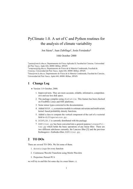
£¤¥Jon Sáenz , Juan Zubillaga ¡ , Jesús Fernández ¢PyClimate 1.0. A set of C and Python routines forthe analysis of climate variability16th October 2000jsaenz@wm.lc.ehu.es, Departamento de Física Aplicada II, Facultad de Ciencias, Universidaddel País Vasco, Apdo 644, 48080–Bilbao, SPAINwmpzuesj@lg,ehu.es, Departamento de Física de la Materia Condensada, Facultad deCiencias, Universidad del País Vasco, Apdo 644, 48080–Bilbao, SPAINchus@wm.lc.ehu.es, Departamento de Física de la Materia Condensada, Facultad de Ciencias,Universidad del País Vasco, Apdo 644, 48080–Bilbao, SPAIN1 Change LogVersion 1.0–October, 2000.¦1. Improved tests. They are more accurate, reliable, informative, comprehensiveand use less disk space.2. The package compiles using distutils. This feature has been checkedon FreeBSD, Linux and OSF platforms.3. Some minor typos corrected in the documentation.4. Added KPDF.c, a extension module to estimate univariate and multivariatekernel–based probability density functions.5. Added a class to compute the vertical component of the curl of a vectorialfield in diffoperators.py.6. DCDFLIB.C is currently distributed with the package.7. KZFilter.py has been converted into a general purpose LinearFilter.pywhich holds the basic operations of any linear filter. There aretwo different subclasses currently, the Lanczos filter [5] and the previousKolmogorov–Zurbenko filter, KZFilter.py.2 TO DOsThere are several TO–DOs. We list some of them:1. docstrings for every function2. Continuous Wavelet Transform using Morlet Wavelets3. Projection–Pursuit PCAwe will try to end this list some day in a near future ;-).1

3 Installation3.1 CompilationVersion 1.0 of pyclimate is distributed using distutils. Thanks to Alberto Garcíafor his help in setting up the setup.py script. After downloading the file PyClimate-1.0.tar.gz, you should decompress, untar and install it. The UNIX commands neededare:gunzip PyClimate-1.0.tar.gztar xf PyClimate-1.0.tarAfter these steps, go into the main directory of pyclimate and a typical installationcommand is:For a general installation (root passwrod required): python setup.py install¦¦For a private installation: python setup.py install home=˜In this last case, you will have to set manually the value of the environmenal variablePYTHONPATH to be able to access pyclimate. The script pyclimatetest.py inthe test directory runs a test that covers many of the routines in the package (seesubsection 3.3).3.2 PrerequisitesMany of the functions developed in this package have been built over other freelydistributed packages and libraries. So, before installing this package, the next softwareis needed:Python interpreter itself, freely available at:¦http://www.python.orgThe Numeric extensions to Python, freely available at:¦http://numpy.sourceforge.netKonrad Hinsen’s Scientific Python, available at:¦hinsenhttp://starship.python.net/crew/§The netCDF library, freely available at:¦http://www.unidata.ucar.eduThe previous version required DCDFLIB.C 1.1 library, too, which is freely availableat: http://odin.mdacc.tmc.edu/anonftp/page 3.html. The currentversion of the package distributes the source and documentation of this library toease the installation of pyclimate. In case the original C files of some of the extensionswere edited, D. Beazley’s SWIG (http://www.swig.org) will be needed to create thePython interface to the C routines. The SWIG source files (*.i) are distributed in thesubdirectory swig.3.3 TestAfter installing the package, a user may be interested in knowing if it is working properly.There is a script which makes extensive use of the functions in pyclimate in2

the subdirectory test. This script (pyclimatetest.py) compares the results obtainedafter the installation with the ones obtained and checked during the developmentand extensive checking of the package. Thus, python pyclimatetest.py runsthe tests and compares the output with the data stored in file reference.cdf. Theoutput of the script is quite informative. Here is shown a excerpt of the output:XG_44_44 |hgt_eofs | : 1.00e-00 dG:-1.11022e-16G_45_45 |hgt_eofs | : 1.00e+00 dG: 2.22045e-16G_46_46 |hgt_eofs | : 1.00e+00 dG: 0.00000e+00XG_47_47 |hgt_eofs | : 1.00e-00 dG:-1.11022e-16RMS Error |hgt_lambdas | : 0.00e+00The first character of each file may be a blank (no difference detected) or a X, inwhich case, a difference has been detected. Most often, these differences are not important,and they are simply due to the fact that the control used is of the type ifrms!=0.0):, which is not accurate enough. The second column shows which is themeasure used to evaluate the differences. Usually, RMS errors are used, but congruencecoefficients (G i i) are also used to evaluate errors in EOFs (and related quantities,like PCs, expansion coefficients for SVD analysis or heterogeneous and homogeneouscorrelation maps) due to the fact that both ¨ and ©¨ are valid solutions of the eigenvalueproblem. The third column states the name of the netCDF variable which holdsthe reference data and the fourth column shows the value of the error measure (RMS orcongruence coefficient). For the special case of congruence coefficients, a last column(dG) shows the difference © to let the user know the real difference for thoselines with a X as the first character.python pyclimatetest.py will usually be called without command line arguments,and it performs the comparisons. However, if a user detects that with herhardware or software she is getting different results (for instance, phases in EOFs) andshe prefers to have her own reference.cdf file, she can use the command lineoption -o to overwrite the reference file. It is not advisable to do this unless the correctnessof pyclimate has been examined at least once after the primary installation inthat platform.3.4 ExamplesThe previous manual included some examples on the use of the code. However, wehave removed those examples from the current version of the manual. They can befound at the directory examples of the distribution. Another different source of informationon the use of the package can be found in the pyclimatettest.py file,which covers most of the functions in the package, using real–life data sets.4 IO functions4.1 ASCII filesThe main goal of file readdat.py is to provide a set of functions to handle IO fromASCII files. The ASCII files must be written in the way gnuplot files are, but notall of the gnuplot–compliant files are readable. Each row in the file is a row of theoutput data. Lines whose first token is a # are comments for these functions. No commentsare allowed at the tail of a line. Empty lines are allowed, but they are discarded3

and not used to separate datasets in the file. Better support for these features existsin other packages for Python, like M. Haggerty’s Gnuplot or the IO functions in K.Hinsen’s Scientific Python. The interest of this file is that it allows to read files withcomplex numbers and other data types, a feature that is not supported by the mentionedfiles. Complex numbers are written as: real,imag, ,imag or real, in the inputfile, with no blank spaces (nor tabs) separating the members of a complex number. Examplesof use of these routines can be found in file exiofuncs.pyFunction: def readdat(fname,typecode=None)Reads all the data in the file fname and returns a bidimensional NumPy array of thesame shape as the data in the original array and with a typecode given as Float64 bydefault (Complex64 in case there were complex elements in the file). If the parametertypecode is explicitly assigned, the output array is coerced to that type.Function: def readcol(fname,col=1,typecode=None)In this case, the col–eth column is read and returned as a one dimensional NumPy array.The numbering of columns is not according to Python’s scheme, but to gnuplot’sone instead, that is, from 1 to N. The type coercion works as in the previous function.Function: def readcols(fname,cols=[1],typecode=None)Similar to readcol, but reads from the file fname and returns a –dimensionalNumPy array, where is the length of the sequence object cols. The type coercionworks as in the previous two functions. The columns are returned in the same order asthey appear in cols.4.2 netCDF filesTo access netCDF files, pyclimate uses the excellent netCDF package in K. Hinsen’sScientific Python. A special function has been built on top of K. Hinsen’sinterface to make the use of structured netCDF files easier, and it is included in filencstruct.py.Function: def nccopystruct(name,inc,dims,vars,varcontents)This function replicates the structure of a Conventions–compliant netCDF file (seeCOARDS conventions http://www.unidata.ucar.edu). These conventionsusually imply the definition of a set of variables like latitude, longitude or vertical leveland some auxiliary attributes like units or the numbers assigned to the missing valuesor scale and offset values for packing. This function helps in the creation of structuredoutput files from an input dataset without having to individually copy ALL of the globalattributes, auxiliary variables and their attributes. In case a history attribute existed,it is updated with the date and the name and arguments of the calling program. Thefunction returns a netCDF file object ready to be used. This function opens the existingnetCDF file with the ’w’ flag, overwriting any existing file with the same name. Parametername is the name of the output datafile to be created. inc is the input NetCDFfile whose structure is to be replicated. dims is a sequence of dimensions of the inputdatafile which are to be copied onto the output datafile. vars is a sequence of variablesto be copied onto the output datafile without copying the contents, just the declaration,type, structure and comments. varcontents is a sequence of variables in the parametervars whose structure and contents are to be copied from the input dataset. The functionexiofuncsnc.py shows examples of use of this function.4

5 Time handling routinesOne of the problems that researchers in climate analysis are usually faced to is theneed to position their observations accurately in time. The file JDTime.py providessome functions to face this problem. It does not intend to provide a complete set ofdate handling routines. In particular, all the computations asume UTC time–zone andno DST functions are included (M.A. Lemburg’s mxDate provides some of these extrafeatures). JDTime.py allows fast, accurate and easy date processing from Pythonwithout the need of extra packages. A very interesting feature is the possibility of easilyusing monthly intervals by means of the function monthlystep(), computed fromthe definition of a tropical year with the same value used in Unidata’s udunits.dat,so that the time values created this way can be correctly read and interpreted by theSDF interface in plotting programs as GrADS. The date arithmetic is carried out bymeans of Julian Days stored as double precision (Float64) numbers. Conversion functionsto date structures are provided by means of a C extension based on astronomicalalgorithms [6]. The file exjdtime.py provides some examples of the use of thesefunctions.Class: JDTimeInteger members: year, month, day, hour, minute.Double member: second.The previous members can be directly accessed from Python.Function: def date2jd(jdt)From a JDTime structure jdt, get the Julian Day number as a double.Function: def jd2date(jd,jdt)Given a Julian Day jd, get the broken date structure jdt.Function: def monthlystep()Return the number of Julian Days in a month, that is, number of tropical days peryear (365.242198781) divided by twelve. This provides adequate accuracy for datesduring the instrumental part of the climate record. However, this approach poses aproblem because of the truncation problem that appears due to the different length ofthe months. When using this approximation, some months are longer than others andthis means that one of the time steps may be in the first day of one month and the laststep on the last day of the same month (if month is longer than 30.43 days). To avoidthis truncation problem, the origin should be set to day 15th of the starting month. Thisway, for every record, the first two fields of the date structure (year and month) will beadequately resolved by jd2date().There is a second file that allows the handling of COARDS compliant time variablesin netCDF files, JDTimeHandler.py.Class: JDTimeHandlerFunction: def init (self,units)The creator parses a COARDS–type units attribute of the netCDF time variable (ex:hours since 1958-01-01 0:0) and computes the offset and the scale factor to get JulianDays from the netCDF time variable for each record.Function: def getdatefields(self,tvalue,listlen=6)This method scales the value of tvalue using the scaling factor corresponding to theunits attribute and adds the offset computed from the units attribute, getting the JulianDay corresponding to the time coordinate tvalue. The Julian Day value is used tocreate a broken date structure, and its values (year,month,day,hour,minute,second) arereturned as a list, with as many members as those requested by listlen.Function: def gettimevalue(self,datefields,listlen=6)5

This function is the inverse of the previous one. It creates a Julian Day from the valuesin the list datefields (as many values as the value of listlen), computes the offset fromthe origin of coordinates and scales the value to the units corresponding to the unitsattribute of the time variable used to cretae the instance of this class. Due to sometruncations which appear during the floating point operations, this function is onlyaccurate to about 12 significant figures. So, if you are creating a netCDF file fromscratch, it is more accurate just to add equal time intervals using a fixed time step fromrecord to record.6 Distribution functionsDCDFLIB.C 1.1 is a library of C Routines for Cumulative Distribution Functions developedby Barry W. Brown, James Lovato and Kathy Russell, Department of Biomathematics,The University of Texas, M.D. Anderson Cancer Center. The library allowsthe determination of cumulative distribution functions, inverses, and the parameters ofthe following statistical distributions: Beta, Binomial, , Noncentral , , Noncentral , Gamma, Negative Binomial, Normal, Poisson, Student’s and Noncentral .The file pydcdflib.py provides access to this library from Python. For each oneof these distributions, a class has been created that wraps the parameters in the callto the functions of this routine and some C functions that wrap the original C callsto make them available to the Python interpreter. The same names have been usedin the wrapping of the parameters, so that the original documentation of the DCD-FLIB.C library is valid for each of the classes in this Python extension. The class ispassed to a function with the same name of the original one (with py prepended tothe name of the wrapper function). The fields of each class are updated by the wrapperfunctions. The code of the original C library is untouched. Examples on the useof these wrappers can be obtained from the testDCDFLIB.py script in the sourcedirectory of the distribution and from the enclosed exdcdflib.py file. There is anerror when computing the parameters for the F distribution using the value which=3.This seems to be linked to the properties of the F distribution and, in case it were abug, it also exists in the original DCDFLIB.C, as the same problem appears using theC file testF.c, provided in the source directory. The documentation of the originalDCDFLIB.C library is distributed within the doc subdirectory of the distribution.7 Simple multivariate statistical toolsThe main goal of file mvarstatools.py is to provide some routines that are beingused by other like svdeofs.py. However, some of them may be interesting bythemselves, and they are thus documented in this section.Function: def center(dataset)Given an input multivariate dataset with arbitrary dimensions (with the restrictionthat first dimension is time), this function returns the centered ! "#©%$ dataset ,$ with the sample $& , average .Function: def standardize(dataset)Given an input multivariate dataset with arbitrary dimensions (with the restriction')(+* (* (.-0/that first dimension is time), this function returns the standardized dataset 132 ,#with 4 *the sample standard deviation 4 *65 ')(768* ( -9/;:

Y

ªIt is distributed as a with G_“¢©@z¤œ)+HaG_“‚©oz¥œ ¦H degrees of freedom. • is the de-Rgrees of freedom of the covariance matrix. lambdas ({ ) are the eigenvalues returnedby svdeofs (array q ) and temporalsamples is the number of temporal samples inthe dataset. The function returns a tuple of arrays (each of them one item shorter thanq ), ( ,“§¨ ). The first element of the tuple is an array with the values of obtainedfrom eqn (1), while the second element holds their probabilities. This test is usuallytoo liberal and tends to overfactor.Function: def northtest(lambdas,temporalsamples)Given as input the eigenvalues lambdas (q from svdeofs) and the number of samplesin the dataset (temporalsamples), tests the degeneracy of eigenvalues accordingŒ~{©]ª h« ¨ , to . It returns the array of ¬cq |­3Œ~{7® values . In case that for a pair of{ ©oŒ~{ ©‘{ R œsŒ~{ R eigenvalues , both members of the pair should be mantainedor removed simultaneously in the factorization [10].Function: def mctesteofs(dataset,eofs,subsamples,length)This function tests, by means of a Monte Carlo test [3], the stability of the EOFs to temporalsubsampling of the original dataset. Given the original dataset, the EOFs of thewhole dataset as returned by svdeofs() (eofs), this function builds several subsampleschosing the records in the original dataset at random. The subsamples are of lengthlength, which must be smaller than the length of the original dataset. The function returnsa Numeric array of shape (subsamples,len(eofs[0])) which holds thecongruence coefficients of the master and perturbed eigenvectors for each subsample.9 SVD of coupled datasetsThe SVD decomposition of the covariance matrix of two datasets is one of the simplest,yet powerful, method to analyze the linear relationship between two coupled geophysicaldatasets [1, 4, 9, 14]. Some functions that implement most of the computationsusually needed for this analysis are provided in the file svd.py. One example on theuse of these functions is in the file testsvd.py.Function: def svd(xfield,yfield)Given two = fields (xfield) > and (yfield), defined as in section 8 (first dimension ofthe array is the temporal one), this function returns the SVD decomposition of theircovariance ¯ *l° ACED , matrix . It returns a tuple of three ± arrays ² , ³ and . Each´ column holds b the –eth singular vector of the (= left ) field. Same convention isfollowed by the ordering of elements ³ in ² . is a one–dimensional array which holdsthe singular 4 values . The singular vectors are (´ Žl´ ^ ‘µ Žlµ ^ ‡Œ Z^ orthonormal )and can be used to linearly project each of the fields to define the expansion coefficientsBGIḨ Ž~´¹ and ºa˜GIH· »FOGIHfŽ;µ whose covariance is the same as the singular“˜GIH·value associated to that mode “I†˜ºl Š ¼4 . The datasets are centered (sample meanis removed) inside the function prior to the SVD computation. The routine does onlywork with two–dimensional fields (first dimension=time axis, second dimension, spatialindex). To avoid this limitation, the user can reshape the data arrays before entering‰this routine to the required 2–D structure and reshape them back to the original one afterthe subroutine.Function: def getcoefs(data,svectors)Given a dataset (= data > or ) and the corresponding set of singular (± vectors or) returned by svd(), this function returns the expansion coefficients (“ or º ) up³to the order stated by the evaluation of len(svectors[0])). This, in fact, meanstruncating the representation of the field at this number. This same approach is used8

11f†˜µ fŠ ) as columns (singular vectors)are in svectors. Each column themaps[:,imap] is the imap–eth map.Function: def heterogeneousmaps(xdata,ycoefs)From the input dataset xdata and the array of expansion coefficients ycoefs, it returnsan array with as many heterogeneous correlation maps ( ‰ >#†“0y Š or ‰ =½†hºly Š )as columns (expansion coefficients) are in ycoefs. The ordering of the maps is as describedin previous routine.Function: def SCF(sigmas)This function returns the squared covariance fraction associated to each singular value,

mented with performance in mind, so that, in order to avoid several iterations througha possibly long dataset, it iterates just once, performing a multivariate filtering to eachrecord. This makes that during the initialization phase, the internal running buffer mustbe initialized (filled) until valid values can be obtained. During the initialization phaseof the filter, this function returns None. After the internal buffer is ready, the functionreturns valid filtered fields until the user arrives at the final record of the iteration.Method: LinearFilter.reset()This method resets the linear filter so that it is able to start computing with a data set ofa different shape avoiding the creation of a new instance of the class.10.1 KZ filter: KZFilter.pyThe Kolmogorov–Zurbenko digital filter is a very simple but powerful digital filter. Itsfeatures are documented elsewhere [7, 12].Class: KZFilterMethod: KZFilter. init (self,points,iterations,lowpass=1)Default (and only) constructor. points is an odd integer representing the number ofpoints in the moving average, while iterations is an integer representing the number oftimes that the average is iterated to get a better damping of the secondary maximums.When the flag lowpass is false, the filter instance works as a high–pass filter.Method: KZFilter.getcoefs(self)This function returns the coefficients that are being used in the filter.Method: KZFilter.cutofffrequency()Returns the approximate cutoff frequency of the filter.10.2 Lanczos filter: LanczosFilter.pyThe Lanczos filter is another very common filter and its mathematical properties andthe algorithms for the compilation of the coefficients can be found for instance at [5].Class: LanczosFilterMethod: LanczosFilter. init (self,filtertype=’bp’, fc1=0.0, fc2=0.5, n=None)Default constructor. filtertype specifies if the filter is low (’lp’), high (’hp’) or band(’bp’) pass. The cut-off frequencies for the bandpass case are set in fc1 and fc2. If thefiltertype is set to ’lp’ or ’hp’ both cut-off frequencies must be equal. Band–pass filterwill be assumed if the frequencies are different, regardless you have specified othertype of filter!The number of different coefficients to be calculated is set with the parameter n. Eventhough it has a default value that is appropiate in the band–pass case, it is stronglyrecommended not to use the default value in any other case (high–pass or low–pass) [5].Method: LanczosFilter.getcoefs(self)As in section 10.1 this function returns the coefficients that are being used in the filter.11 Differential operators: diffoperators.pySome routines to compute differential operators on the sphere specially suited for climateanalysis are provided. By now, they only process two–dimensional fields andregular latitude–longitude grids. The operators make the computations by means ofcentered differences, except at the borders, where they use backward or forward differences(no periodic boundary conditions supported yet). All the operators assume that10

R-—ÁÄ.ÅhÆ;Ç : 68ÌÇÈ—Á-RÓ-Ì6Ë ÇÈRÈthe input fields are organized according to the COARDS scheme ([latindex,lonindex]).Class: HGRADIENTMethod: HGRADIENT. init (self,lats,lons,asdegrees=1)This is the constructor for the horizontal gradient calculator. lats is a NumPy arraywhich holds the latitudes corresponding to the grid points, lons holds the longitudes ofthe grid points and if the optional parameter asdegrees is set to true, it means that theinput angular variables are expressed as degrees, not radians.Method: HGRADIENT.hgradient(self,hfield,R=6.37e6)Given as input the horizontal field ( hfield ), get as a result a tuple which holds thezonal and meridional components of the gradient on the sphere ÃÄ.ÅhÆ3ǤÈ+ÉÈ «( , ßÈ+ÉÇ ). Ris assigned by default the radius of the Earth.Class: HDIVERGENCERMethod: HDIVERGENCE. init (self,lats,lons,asdegrees=1)Default constructor, with parameters defined as for the gradient operator.Method: HDIVERGENCE.hdivergence(u,v,R=6.37e6)From the zonal (u) and meridional (v) components of a vectorial field, find the horizontaldivergencewith the divergence field.Class: VCURLÊ È+ËÈÃÄ.ŘÆ3Ç«œ ÈÍ . The function returns a bidimensional arrayMethod: VCURL. init (self,lats,lons,asdegrees=1)Default constructor, with parameters defined as for the gradient operator.Method: VCURL.vcurl(u,v,R=6.37e6)From the zonal (u) and meridional (v) components of a vectorial field, find the verticalcomponent of the curl operator on the © È Í sphere,. The functionreturns a scalar field with the vertical component of the curl of the vectorial field.ÈÈÃÎÄ.ŘÆ;ÇsÊ«Ä.ÅhÆ+Ç :12 Multivariate and Univariate Kernel based ProbabilityDensity Function Estimation: KPDF.cHistograms are useful and simple estimators for the Probability Density Function (PDF)associated with physical or modelling experiments. However, the estimation of PDFsby means of histograms presents some drawbacks like the instability to the selectionof the bins (bin number and bin origin) or the lack of derivability. Thus, it has beenproposed [13] the use of a kernel based approach to the estimation of the PDF. Thismodule provides functions to perform univariate and multivariate PDF estimation. Therelevant equations for this module are 2 for univariate density estimation and 3 formultivariate series.„Ð Ÿ©o=І (2)ÏG9HfRILRÑ]ÒV

Returns a NumPy array with the PDF associated to the experimental data edata evaluatedat points gdata (NumPy array, too) using a bandwidth h. For this and next functions,edata and gdata must be NumPy arrays and the function returns a NumPy arrayof typecode Float64. The kernel used in the estimation is a Epanechnikov one. It raisesTypeError if edata or gdata is not a 1-D NumPy array It raises MemoryError ifit is unable to allocate the returned array or some temporal arrays which are needed asworking space.Function: def UPDFBiweight(edata,gdata,h)Same as the previous function, but use a biweight kernel, instead (S86, Table 3.1). Itraises TypeError if edata or gdata is not a 1-D NumPy array It raises MemoryErrorif it is unable to allocate the returned array or some temporal arrays which areinternally needed as working space.Function: def UPDFTriangular(edata,gdata,h)Same as the previous function, but using a triangular kernel function (see S86, Table3.1) It raises TypeError if edata or gdata is not a 1-D NumPy array It raisesMemoryError if it is unable to allocate the returned array or some temporal arrayswhich are internally needed as working space.Function: def UPDFOptimumBandwidth(edata)Get an approximation to the optimum bandwidth by means of equation 3.28 (S86). Unlessthere is a better suggestion, it can be a good starting point. edata is, as previously,a NumPy array (internally works as Float64). It raises ValueError if edata is not asource sequence.Function: def MPDFEpanechnikov(edata,gdata,h,Sm1=None,K=0.0)Given a multidimensional (dimension “&Û¡\ ¦E†˜Ü ` currently) experimental data set edata(NumPy array), evaluate the PDF at each “ -dimensional point in the NumPy arraygdata, using a radially symmetric bandwidth Ð . The optional parameter Sm1 is a“!mΓmatrix (NumPy array, too) which can be used to scale each of the directions in theedata and gdata arrays. Usually, the inverse of the covariance matrix of edata is agood selection for this parameter. It can also be None, in which case, no scaling isapplied to the directions in the “ –dimensional space. K is a renormalizing constantwhich must be computed according to the scaling defined by Sm1. If the inverse ofthe covariance matrix is selected as Sm1 and the square root of the determinant of thecovariance matrix is input as K, then, a Fukunaga estimator is being used in the estimation(S86, Eq. 4.7). This function uses a multidimensional Epanechnikov kernel(S86, Eq. 4.4) for the estimation. It raises ValueError if edata or gdata are notNumPy arrays. It raises TypeError if h is not a number. It raises ValueError ifthe dimensionality of the data sets edata and gdata is not correct because they exceedthe implemented capability, they are not ”compatible” (for instance, one is 2-D and theother one 3-D), or the scaling matrix is not the adequate range (“&mc“ ).Function: def MPDFGaussian(edata,gdata,h, Sm1=None, K=0.0 )Same as MPDFEpnechnikov, but using a Gaussian multivariate kernel (S86, Eq. 4.3).It raises ValueError if edata or gdata are not NumPy arrays. It raises TypeErrorif h is not a number. It raises ValueError if the dimensionality of the data sets edataand gdata is not correct because they exceed the implemented capability, they are not”compatible” (for instance, one is 2-D and the other one 3-D), or the scaling matrix isnot the adequate range (“&m!“ ).Function: def MPDFOptimumBandwidth(edata)Provides a first guess to the optimum bandwidth (S86, Eq. 4.14). It raises ValueErrorif edata is not a source sequence or if its dimensions exceed current capabilities.Function: def MPDF2DGrd2Array(xdata,ydata,fastestdim=0)12

This function returns an array of shape (len(xdata)*len(ydata),2) whichholds in a linear fashion the grid defined by arrays xdata and ydata. The optionalparameter fastestdim allows the selection of the dimension which grows faster (outerone by default) or inner one if it is non zero.Function: def MPDF3DGrd2Array(xdata,ydata,zdata,fastestdim=0)This function s similar to MPDF2DGrd2Array in the sense that it returns an arrayshape like (len(xdata)*len(ydata)*len(zdata),3) which holds in a linearfashion the grid defined by arrays xdata, ydata and zdata. The optional parameterfastestdim allows the selection of the dimension which grows faster (outer one bydefault) or inner one if it is non zero.13 Other linksThere are other packages that can be combined with Python, pyclimate, and theother packages that have been mentioned previously and which allow to easily buildpowerful data analysis tools and programs. To name a few, for graphics, for instance,there exists the posibility of using DISLIN (http://www.linmpi.mpg.de/dislin/),free for some platforms. There is another set of statistical functions by G. Strangman(http://www.nmr.mgh.harvard.edu /Neural Systems Group/gary/python.html). Acomplete repository of Python programs can be found at the official WEB server(http://www.python.org) or Starship, (http://starship.python.net) the server for the communityof Python contributors and developers.References[1] C. S. Bretherton, C. Smith, and J. M. Wallace. An intercomparison of methodsfor finding coupled patterns in climate data. J. Climate, 5:541–560, 1992.[2] C. E. Buell. The number of significant proper functions of two–dimensionalfields. Journal of Applied Meteorology, 17(6):717–722, 6 1978.[3] X. Cheng, G. Nitsche, and J. M. Wallace. Robustness of low–frequency circulationpatterns derived from EOF and rotated EOF analyses. J. Climate, 8:1709–1713, 1995.[4] S. Cherry. Singular value decomposition analysis and canonical correlation analysis.J. Climate, 9:2003–2009, 9 1996.[5] C. E. Duchon. Lanczos filtering in one and two dimensions. J. Appl. Met.,18:1016–1022, 1979.[6] P. Duffet-Smith. Practical Astronomy with your Calculator. Cambridge UniversityPress, 3 edition, 1990.[7] R. E. Eskridge, J. Y. Ku, S. T. Rao, P. S. Porter, and I. G. Zurbenko. Separatingdifferent scales of motion in time series of meteorological variables. Bulletin ofthe American Meteorological Society, 78(7):1473–1483, July 1997.[8] J.E. Jackson. A User’s Guide to Principal Components. Wiley Series in Probabilityand Statistics. Applied Probability and Statistics. John Wiley & Sons., 1991.13

[9] M. Newman and P.D. Sardeshmukh. A caveat concerning singular value decomposition.J. Climate, 8:352–360, 1995.[10] G.R. North, T.L. Bell, R.F. Cahalan, and F.J. Moeng. Sampling errors in the estimationof empirical orthogonal functi ons. Monthly Weather Review, 110:699–706, July 1982.[11] R. Preisendorfer and C.D. Mobley. Principal Component Analysis in Meteorologyand Oceanography. Developments in Atmospheric Science. Elsevier, Amsterdam,1988.[12] S. T. Rao, I. G. Zurbenko, R. Neagu, P. S. Porter, J. Y. Ku, and R. F. Henry. Spaceand time scales in ambient ozone data. Bulletin of the American MeteorologicalSociety, 78(10):2153–2166, October 1997.[13] B. W. Silverman. Density Estimation for Statistics and Data Analysis. Chapmanand Hall, Londres, 1986.[14] H. von Storch and A. Navarra, editors. Analysis of Climate Variability. Applicationsof Statistical Techniques. Springer, Berlin, 1995.14