Momenta of a vortex tangle by structural complexity analysis

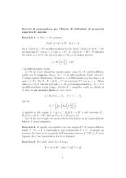
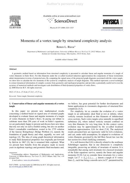
Author's personal copy2224 R.L. Ricca / Physica D 237 (2008) 2223–2227Fig. 1. The area A of the projected graph resulting from the projection p ν ofa vortex line L on the plane Π is proportional to the component of the linearmomentum of L in the ν-direction.arc-length s. Vorticity ω is defined on L i , and is simply given byω = ¯ωX ′ , where, in general, X = X(s, t) denotes the positionvector, ¯ω a constant and t ≡ X ′ the unit tangent to L i (the primedenoting the derivative with respect to s, and t is time). Thelinear momentum P = P(T ) corresponds to the hydrodynamicimpulse, which generates the motion of T from rest, and fromits standard definition [11] takes the formP = 1 ∫X × ωd 3 X = 1 N∑Γ i X × X2 T2i=1∫L ′ ds, (1)iwhere P is here intended per unit density, and Γ i representsthe circulation of L i . Similarly, for the angular momentumM = M(T ), that corresponds to the moment of the impulsiveforces acting on T ; we haveM = 1 ∫X × (X × ω)d 3 X3 T= 1 N∑Γ i X × (X × X3∫L ′ )ds, (2)ii=1where, again, M is intended per unit density. We remark thatunder both Euler’s equations and LIA, we havedPdt= 0,dMdt= 0. (3)2. Interpretation of momenta in terms of projected areaArms and Hama [8], who first proved the conservation ofthe integral on the right-hand side of Eq. (1) for a single vortexline, showed that this quantity admits interpretation in terms ofprojected area (see Fig. 1). Indeed, by direct inspection of theintegrand above, it is evident that under LIA the plane projectedarea of the vortex line is proportional to the component ofthe linear momentum of the vortex along the direction ofprojection.Let p = p ν denote the orthogonal projection onto the planeΠ along the direction ν, and L ν = p ν (L) be the graph diagramof a smooth space curve L under p ν . Evidently L ν depends onν. For the moment let L ν be a smooth planar curve with noself-intersections, but in general L ν will be a nodal curve withself-intersections, the latter resulting from the projection of theapparent crossings of L, when L is viewed along the line ofsight ν.By identifying the vortex line with its geometric support L,the projected graph diagram L ν will be oriented, the orientationbeing naturally induced by the vorticity vector. Let L xy , L yz ,L zx be the three graph diagrams of the projected vortex lineonto the mutually orthogonal planes x = 0, y = 0, z = 0,and let A xy = A(L xy ), A yz = A(L yz ), A zx = A(L zx ) be thecorresponding areas of the plane regions bounded by L xy , L yz ,L zx , respectively.By applying the results of Arms and Hama [8], from (1) wehaveP xy = Γ A xy , P yz = Γ A yz , P zx = Γ A zx , (4)where Γ is vortex circulation. Moreover:Definition 2.1. The resultant area A max is the maximal areaobtained by max ν p(A) = p max (A) (along the resultant axisν max ) among all possible projected areas A.The direction of the resultant axis ν max is clearly that of thelinear momentum. Hence, also from [8], we haveTheorem 2.2 (Maximal Area Interpretation). The resultantlinear momentum of a vortex line L, of circulation Γ , underLIA is given by P = Γ A max ν max , where A max is the resultantarea. The projected area of L on any plane perpendicular tothat of the resultant area is zero.Similar results hold true for the angular momentum. Withreference to the right-hand side of Eq. (2), the second integralcan be interpreted in terms of areal moment, according to thefollowing definition:Definition 2.3. The areal moment around any axis is theproduct of the area A multiplied by the distance d betweenthat axis and the axis a G , normal to A through the centroidG of A.For a vortex line L, the centroid G of the projected area A isthe center weighted with respect to the vorticity distribution ofL. As for the linear momentum, the components of the angularmomentum are determined by the areal moments:M xy = Γ d z A xy , M yz = Γ d x A yz , M zx = Γ d y A zx , (5)where evidently d x , d y , d z are the distances between therotational axis and the centroid axes through A yz , A zx , A xy ,respectively. Similar considerations apply to define the resultantareal moment of L:Definition 2.4. The resultant areal moment of L is the arealmoment around the resultant axis a G of the projected areas ofL onto two mutually orthogonal planes, parallel to a G .⋃These observations are easily extended to a tangle T =i L i of N vortex lines L i , provided we carefully define the

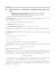
Author's personal copyR.L. Ricca / Physica D 237 (2008) 2223–2227 2225Fig. 2. (a) The number in the dashed region is the value of the index I P (C) according to the right-hand rule convention and the algebraic intersection numbercalculated by Eq. (6). (b) The oriented nodal curve, resulting, for example, from the standard projection of a figure-8 knot, has 5 bounded regions. Note that one ofthe interior regions has index 0, due to the opposite orientation of the strands crossed by ρ. (c) Contribution from each A(R j ) must be weighted according to thecirculations on the boundary ∂R j .area of the resulting oriented graph diagram. The difficulty hereis precisely in the correct calculation of such area.3. Signed area of oriented graph diagramsThe oriented graph diagram of a tangle of vortex linesis an oriented nodal curve (i.e. the “underlying universe”of the tangle) in R 2 , and this can easily attain considerablecomplexity, particularly as regards the localization of selfintersections.A necessary first step is to reduce nodal curves ofany complexity to good nodal curves, that have (at most) doublepoints. Nodal points are classified according to their degree ofmultiplicity µ(P) given by the number of arcs incident at thepoint of intersection P. If P is a double point, then µ(P) = 2.If P is a point of multiplicity µ(P) = n (n > 2), we can alwaysreduce its multiplicity by “shaking” the graph diagram (actuallyits pre-image) near P to get m = 1 2 (n2 − n) double points, byvirtual perturbations of the incident arcs from their location.Thus, if h (n) is the total number of points of multiplicity n, byapplying this shaking technique we can always replace theseh (n) points with h(n) = mh (n) (m ≥ 3) double points. We saythat a graph diagram is a good projection, when it has at mostdouble points. Hence, by the shaking technique, we can alwaysreduce highly complex graph diagrams to good nodal curves.Let C denote one such good nodal curve on Π , and let A(C)be the corresponding total area. In order to calculate this area,first we need to define the index I P (C) of C at the point P (forthis see, for example, [12]). Let P ∉ C, t the tangent to C and ρthe radiant vector with foot at P, that intersects C transversally.At each intersection point X ∈ ρ ∩ C assign the algebraicsign ɛ(X) = ±1, according to the standard convention givenby the right-hand rule, that is ɛ(X) = +1 when the frame{ρ, t} is positive (see Fig. 2(a)). If X is a double point, thenthe intersection is computed with one of the neighbouring pairsof the incident, equi-oriented arcs.Definition 3.1. The index I P (C) of C at P is the algebraicintersection number given byI P (C) =∑ɛ(X). (6)X∈ρ∩CHence, I P (C) ∈ Z.Let us now consider the Z sub-domains {R j } j=1,...,Zdetermined by C ∩ Π and bounded by C, and let A(R j ) > 0denote their standard area. Since every point P ∈ R j has thesame I P (C), we shall call I j the index associated with anypoint P ∈ R j and assign this value to each sub-domain R jof C ∩Π (see Fig. 2(b)). The signed area of an oriented graph, aconcept that can be traced back to Gauss [13], is thus given bythe following rule.Rule 3.2 (Signed Area). The signed area A(C) of an oriented,planar nodal curve C, is given byA(C) =Z∑I j A(R j ), (7)j=1where A(R j ) > 0 is the standard area of R j .4. Linear and angular momenta of a vortex tangle bystructural complexity analysisBy the signed area rule we can calculate the projectedarea of any nodal curve, be it the graph of a single vortexline, or that of a complex tangle of vortices. If the vorticeshave different circulations, a weighting factor defined in termsof contributions from each arc of ∂R j must be assigned toA(R j ) (see Fig. 2(c)). The simplest correction comes from thealgebraic weighting γ j . Let L j = L(∂R j ) = ∑ k=1,...,M L k, jdenote the total length of the boundary curve ∂R j made of Moriented arcs, the k-th arc having length L k, j and circulationΓ k . We haveDefinition 4.1. The circulation weighting factor γ j of R j isgiven byγ j =M∑Γ k L k, jk=1L j. (8)If all the vortices have same circulation Γ , then evidentlyγ j = Γ . Appropriate weighting of circulation is necessary todetermine the correct location of the centroid of the projectedarea. To summarize, we have the following result.

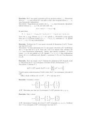
Author's personal copy2226 R.L. Ricca / Physica D 237 (2008) 2223–2227Theorem 4.2 (Signed Area Interpretation). Let T be a vortextangle evolving under LIA. Then, the linear momentumP = P(T ) has componentsP xy =Z∑γ j I j A xy (R j ), P yz = · · · , P zx = · · · , (9)j=1and the angular momentum M = M(T ) has componentsM xy = d zZ∑γ j I j A xy (R j ), M yz = · · · , M zx = · · · ,(10)j=1where A xy (R j ), . . . , etc. denotes standard area of R j .Proof of the above theorem is based on direct applications of(4) and (5), by using the signed area Rule 3.2.5. Dynamical aspects based on signed area informationSigned area contributions provide useful information, thatcan be applied, predictively, to estimate and, postdictively,to understand some dynamical properties of the system.Remember that: (i) areas with index 0 do not contributeto the momentum; (ii) areas with high index (in absolutevalue) weight more and, proportionally, contribute more tothe dynamical impulse of the system; (iii) areas of oppositesign determine contributions in opposite directions. Additionalinformation on dynamical aspects may also come from indexgradient analysis. Take the case of Fig. 2(b): here the alignmentof regions, where the index gradually changes from −1 to +2,indicates the presence of a principal axis of revolution. Theexact location of this axis, placed orthogonally to the alignmentof such regions, is determined by an accurate estimate of theweighted areas and, in any case, it can be determined by signedarea information.Let us consider two other examples, assuming, forsimplicity, equal circulations and maximal projected areas. InFig. 3(a) we have the projection of a single coiled filament, thatin space is wound up 5 times around a circular axis (not shown).Contribution from the 5 negative areas exceeds that from thepositive area, hence the resultant momentum is oriented inthe negative direction. If such a vortex configuration existed,it would propagate backwardly in space. Such an unusualbehaviour may not be so unrealistic, as recent analyticalsolutions [14,15] and numerical tests [16] seem to suggest.Another interesting case is illustrated by the followingexample. Consider the head-on collision of two anti-parallelvortex rings, propagating co-axially one against the other.The linear momentum of the two-ring system (as a whole) isobviously zero, and in ideal conditions this value is conserveduntil collisional time. In the case of real dynamics at sufficientlyhigh Reynolds number, slight perturbations of the circularaxes are likely to develop and, upon collision, we can expectthat these will trigger sinusoidal disturbances along the twocolliding ring axes. Here, analysis of the projected diagrammay be rather illuminating. Without loss of generality and forthe sake of simplicity, let us drastically simplify the situationand consider the perturbed circular axes as the elliptical curvesFig. 3. (a) Projected diagram of a coiled vortex filament: contribution fromnegative areas (light grey) exceeds that from positive area (dark grey); hence,the resultant linear momentum of the vortex is negative. (b) Graph of theprojection of two anti-parallel, elliptical vortex rings: opposite contributionsfrom regions of index of alternating sign (light grey) cancel out; hence, theresultant linear momentum of the two-ring system is zero.sketched in Fig. 3(b) (realistic perturbations would obviouslygenerate a far more complex diagram). The central regionhas index 0 and is surrounded by four regions (light grey) ofalternating sign. Consistently with what we expect from theannihilation of the rings velocity, this gives zero contributionto the resultant linear momentum of the two-ring system.When the two rings collide, the alternating sign of the foursurrounding regions is an indicator of an imminent structuralinstability, that produces the shoot-off of a pair of smallvortex rings on either side of the collisional plane. In arealistic scenario, the precise number of surrounding regionswill depend on geometric details of the perturbation, but inany case the production of an equal number of secondarysmall rings on either side of the collisional plane must beexpected. These considerations seem confirmed by directinspection of experimental results (see, for instance, [17]). Inreal experiments a diadem of a large number of secondarysmall vortex rings is clearly visible. This diadem grows fromthe instability of a fluid membrane that is produced in thecollisional plane, upon collision of the primary large vortexrings. These secondary rings appear to be alternately distributedon either side of the collisional plane, surviving just for a shorttime before final dissipation.6. Concluding remarksThe geometric method based on the signed area interpretationsummarized by Theorem 4.2 provides a new and potentiallyuseful tool for fluid dynamics research. The method exploitsinformation from structural complexity analysis of a tangleof vortex filaments to estimate linear and angular momentaof the system. This is done by computing the signed areas ofthe projected graph diagrams associated with the vortex tangle,

Author's personal copyR.L. Ricca / Physica D 237 (2008) 2223–2227 2227after application of appropriate shaking and weighting techniques.The results are rigorously valid in the LIA context, but,as mentioned earlier, in principle they could be extended to thinvortex filaments governed by the Biot–Savart law. This extensionseems plausible as long as vorticity remains localized in atubular domain of volume small compared with the fluid volume‘embraced’ by the tangle. In terms of projected areas, thiscorresponds to assuming that the (standard) area of the vorticitydomain is much smaller compared with the overall area enclosedby the outermost boundary projected curve, the order ofapproximation depending presumably on this ratio. Physically,this simply means that the higher the localization of vorticity,the most efficacious is the production and transfer of hydrodynamicimpetus and moment, two quantities that are conservedunder Euler’s equations, regardless of the validity of the localizedinduction approximation.In any case, for LIA systems the geometric method proposedhere provides a potentially useful tool for predictive andpostdictive diagnostics. By analyzing projected areas, it canbe applied to implement tests of accuracy of numericalmethods simulating vortex tangles. In superfluids, in particular,by analyzing the area distribution of the vortex projectionone can judge about the scale distribution of linear andangular momenta, and compare this with the expectedvalues of the spectrum of turbulence (Kolmogorov’s twothirdslaw). Moreover, since LIA preserves an infinity ofinvariants of motion, all of these admitting a geometricinterpretation in terms of global curvature, torsion and higherordergradients [18,10], these can be implemented to supplyfurther information on dynamical properties (for instance,kinetic energy and helicity). Other features associated with theanalysis of projected graphs can be related to dynamical issues,but this is beyond the scope of this article. We just like toconclude mentioning that the famous relation [19] χ(G) =v − e + r, between the Euler characteristic χ(G) of a graphG (associated with vortex topology), of v vertices, e edgesand r regions, may find also useful applications in the studyof complex systems [20] and in the advanced diagnostics ofcomplex flow patterns.AcknowledgmentsI would like to thank C. Weber for pointing out Ref. [13].Financial support from Italy’s MIUR (D.M. 26.01.01, n. 13“Incentivazione alla mobilità di studiosi stranieri e italianiresidenti all’estero”) and from ISI-Fondazione CRT (LagrangeProject) is kindly acknowledged.References[1] L. Euler, Solutio problematis ad geometriam situs pertinentis, CommentariiAcademie Scientiarum Imperialis Petropolitanae 8 (1741) 128–140.[2] G.L. Alexanderson, Euler and Königsberg’s bridges: A historical view,Bull. Am. Math. Soc. 43 (2006) 567–573.[3] Lord Kelvin (W. Thomson), On vortex atoms, Proc. R. Soc. Edin. 6 (1867)94–105.[4] C.F. Barenghi, R.L. Ricca, D.C. Samuels, How tangled is a tangle?Physica D 157 (2001) 197–206.[5] R.L. Ricca, Structural complexity, in: A. Scott (Ed.), Encyclopedia ofNonlinear Science, New York and London, Routledge, 2005, pp. 885–887.[6] K.W. Schwarz, Three-dimensional vortex dynamics in superfluid 4 He:Homogeneous superfluid turbulence, Phys. Rev. B 38 (1988) 2398–2417.[7] L.S. Da Rios, On the motion of an unbounded liquid with a vortexfilament of any shape, Rend. Circ. Mat. Palermo 22 (1906) 117–135(in Italian).[8] R.J. Arms, F.R. Hama, Localized induction concept on a curved vortexand motion of an elliptic vortex ring, Phys. Fluids 8 (1965) 553–559.[9] Y. Fukumoto, On integral invariants for vortex motion under the localizedinduction approximation, J. Phys. Soc. Japan 56 (1987) 4207–4209.[10] R.L. Ricca, Physical interpretation of certain invariants for vortex filamentmotion under LIA, Phys. Fluids A 4 (1992) 938–944.[11] P.G. Saffman, Vortex Dynamics, Cambridge University Press, Cambridge,1991.[12] R. Langevin, Differential geometry of curves and surfaces, in: R.L. Ricca(Ed.), An Introduction to the Geometry and Topology of Fluid Flows,in: NATO Science Series II, vol. 47, Kluwer Academic Publs., Dordrecht,2001, pp. 13–33.[13] C.F. Gauss, Letter to H. Olbers, Werke 8 (1825) 398–400.[14] Y. Fukumoto, Stationary configurations of a vortex filament in backgroundflows, Proc. R. Soc. Lond. A 453 (1997) 1205–1232.[15] L. Kiknadze, Yu. Mamaladze, The waves on the vortex ring in He II, J.Low Temp. Phys. 126 (2002) 321–326.[16] C.F. Barenghi, R. Hänninen, M. Tsubota, Anomalous translationalvelocity of vortex ring with finite-amplitude Kelvin waves, Phys. Rev. E74 (2006) 1–5.[17] T.T. Lim, T.B. Nickels, Instability and reconnection in head-on collisionof two vortex rings, Nature 357 (1992) 225–227.[18] H.K. Moffatt, R.L. Ricca, Interpretation of invariants of the Betchov–DaRios equations and of the Euler equations, in: J. Jimenez (Ed.), The GlobalGeometry of Turbulence, Plenum Press, New York, 1992, pp. 257–264.[19] W.S. Massey, Algebraic Topology: An Introduction, Harcourt, Brace andWorld, Inc., New York.[20] R.L. Ricca, Structural complexity and dynamical systems, in: R.L. Ricca(Ed.), Lectures on Topological Fluid Mechanics, Springer-CIME LectureNotes in Mathematics, Springer-Verlag, Berlin, 2008 (in press).