UIC comfort tests - VTI
UIC comfort tests - VTI
UIC comfort tests - VTI

You also want an ePaper? Increase the reach of your titles
YUMPU automatically turns print PDFs into web optimized ePapers that Google loves.
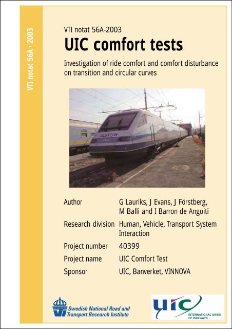
<strong>VTI</strong> notat 56A • 2003<strong>VTI</strong> notat 56A-2003<strong>UIC</strong> <strong>comfort</strong> <strong>tests</strong>Investigation of ride <strong>comfort</strong> and <strong>comfort</strong> disturbanceon transition and circular curvesAuthorG Lauriks, J Evans, J Förstberg,M Balli and I Barron de AngoitiResearch division Human, Vehicle, Transport SystemInteractionProject number 40399Project nameSponsor<strong>UIC</strong> Comfort Test<strong>UIC</strong>, Banverket, VINNOVA
PrefaceDuring 1988 the Director of <strong>UIC</strong> High Speed Division, Mr Maraini, asked MrLauriks to organise a meeting to discuss the “Improvement of passenger trainperformances on conventional lines”. This meeting resulted later in a workinggroup called “<strong>UIC</strong> Comfort Group” to organise a test with a tilting train toinvestigate ride <strong>comfort</strong> and <strong>comfort</strong> disturbances on transition curves as well ason circular curves. Investigation on ride <strong>comfort</strong> on straight lines had beeninvestigated by ERRI earlier.The <strong>comfort</strong> test was then performed by Trenitalia with a Pendolino“Cisalpino” pre-series train from Alstom on the line between Firenze and Arezzoin October 2001. Trenitalia did the recordings of the measured data and a firstevaluation. Main analysis was done by Mr J Evans and a second opinion on theanalysis was done by Dr. J. Förstberg, <strong>VTI</strong>. Mr Lauriks wrote the main body ofthis report.Participants in the <strong>UIC</strong> working group on <strong>comfort</strong>Mr G. LAURIKS (SNCB ) – ChairmanMs M. BALLI (FS – TRENITALIA)Mr I. BARRON DE ANGOITI (<strong>UIC</strong>)Mr P. COSSU (FS – TRENITALIA)Mr J. EVANS (AEA TECHNOLOGY RAIL)Dr J. FÖRSTBERG (<strong>VTI</strong>)Dr K KUFVER (<strong>VTI</strong>) (1999–2001)Mr H. GÅSEMYR (JBV)Mr TH. KOLBE (DBAG)The <strong>UIC</strong> working group started work on 07/10/1999The work was completed on 16/01/2003.<strong>VTI</strong> notat 56A-2003
ContentsPageAbbrivations and Notations 71 Summary 91.1 Requirements 91.1.1 History 91.1.2 Situation before the now completed <strong>tests</strong> 91.1.3 Remaining requirements 91.2 Origin of the work 91.3 Preparation of the <strong>tests</strong> 101.3.1 Characteristics of the potential participating trains 101.3.2 Results of the simulation 101.3.3 Test plan 101.4 Execution of the <strong>tests</strong> 101.5 Preparation of the data for analysis 111.6 Analysis 111.7 Validity of the conclusions 111.8 Conclusions 111.8.1 Consideration 111.8.2 Models 122 Purpose of the study 133 What does <strong>comfort</strong> mean in the context of this report? 143.1 Introduction 143.2 Comfort types 143.3 Comfort index 153.4 Comfort aspects 153.4.1 General 153.4.2 General aspects of passengers’ <strong>comfort</strong> estimates 163.4.3 Influence of time 174 How <strong>comfort</strong> evolves with speed 184.1 On straight track 184.2 On curved track 184.2.1 Non-tilting trains 184.2.2 Tilting trains 185 Elements of dis<strong>comfort</strong> 195.1 On straight track 195.2 On curved track 195.2.1 General definitions 195.2.2 Theoretical behaviour of those disturbing factors 225.2.3 Compensation of lateral acceleration dis<strong>comfort</strong> in circularcurves 236 Actual evaluation rules 266.1 Evaluation of <strong>comfort</strong> on straight track 266.2 Evaluation of <strong>comfort</strong> on curved track 266.2.1 Comfort at curve transitions 266.2.2 Comfort at discrete events 276.3 Statistical interpretation of experimental results 27<strong>VTI</strong> notat 56A-2003
6.3.1 General 276.3.2 Application in the case of <strong>comfort</strong> investigation 287 Choice of the test zone 307.1 Choice of the test route 307.1.1 Evaluation of the offered routes 307.2 Selection of Test Zones 317.3 Quality of the track in the test zone 338 Description of the test 348.1 The train 348.2 Main features of ETR 470.0 348.3 Measured parameters 348.3.1 Measured signals 348.3.2 Vote registration 358.3.3 Synchronisation between votes at different locations in thetrain 368.3.4 Synchronisation of the votes and the track sections to bejudged 368.4 Test conditions 368.4.1 Route 368.4.2 Test runs 368.4.3 Test subjects 378.5 Registration of data, calculation of parameters 388.5.1 Method 388.5.2 Comment 388.6 Measurements for <strong>comfort</strong> 398.6.1 Location and type of sensors 398.6.2 Occupied places 409 Possible influences of construction concepts of vehicle,track and/or system functioning on <strong>comfort</strong> 419.1 Introduction 419.2 Basis for the examples in this chapter 419.3 Study of the car body angle 429.3.1 Influence of vehicle length 429.3.2 Influence of the flexibility of the suspension 429.4 Influence on lateral forces 439.4.1 Influence of the dynamic behaviour 439.4.2 Influence of length of the coach 449.4.3 Influence of position in coach 459.4.4 Additional dis<strong>comfort</strong> due to functioning servo mechanisms 4610 General evaluation of local <strong>comfort</strong> results 4710.1 Evaluation of votes 4710.1.1 Conclusions 4810.1.2 Remark 4810.2 Variation between groups 4810.2.1 Significance of the difference 4910.3 Seat position 5010.4 Track elements 5110.5 Evaluation of measured data 53<strong>VTI</strong> notat 56A-2003
10.5.1 Transitions 5311 Evaluation of local <strong>comfort</strong> 6011.1 Analysis of Transition response 6011.1.1 Types of transition 6011.1.2 Test Conditions 6011.1.3 Parameters 6111.1.4 Scaling of votes 6211.1.5 Examination of votes 6211.1.6 Examination of data – simple transitions 6211.1.7 Relationship between parameters – simple transitions 6411.1.8 Regression analysis – simple transitions 6811.1.9 Investigation of leading vehicle effects 7211.1.10 Effect of other transition types 7311.1.11 Non-linear regressions 7811.1.12 Regression for track engineers 7811.1.13 Contribution of diverse regression parameters 7911.1.14 Estimation of group effect, knowing the regression model 8111.1.15 Estimation of the residual influence of the position in thevehicle 8411.1.16 Linear estimations of the test subjects 8511.1.17 Study of the errors: Measured-Estimation 8711.1.18 Conclusions on <strong>comfort</strong> in curve transitions 8811.2 Analysis of Circular curves 8811.2.1 Test Conditions 8811.2.2 Parameters 8911.2.3 Scaling of votes 8911.2.4 Examination of data 8911.2.5 Relationship between parameters 9111.2.6 Regression analysis 9211.2.7 Regressions with Reduced Dataset 9511.2.8 Conclusion on <strong>comfort</strong> in circular curves 9812 Evaluation of average <strong>comfort</strong> 9912.1 Analysis of average <strong>comfort</strong> 9912.1.1 Test Conditions 9912.1.2 Parameters 9912.1.3 Scaling of votes 10012.1.4 Examination of data 10012.1.5 Relationship between parameters 10112.1.6 Regression analysis 10412.2 Discussion of the results 10712.2.1 Preliminary Conclusion 10712.2.2 General quality of the regression 10712.2.3 Spread of the errors 10812.2.4 Average error per place in train. 10812.2.5 Density of importance of each parameter 10912.2.6 Cumulative importance of each parameter 10912.2.7 Conclusions 109<strong>VTI</strong> notat 56A-2003
13 Conclusions 11013.1 Conditions 11013.1.1 Environmental conditions of the <strong>tests</strong> 11013.1.2 Extrapolation of results. 11013.1.3 Calculation procedure 11013.2 General impressions on the quality 11013.2.1 The <strong>comfort</strong> evaluation is linear in the conditions coveredby the <strong>tests</strong> 11013.2.2 The description of the <strong>comfort</strong> is sufficiently good todescribe the <strong>comfort</strong> differences due to the seat position 11013.3 Conclusions in relationship with the organisation of <strong>tests</strong> 11113.3.1 Choice of the test track 11113.3.2 Choice of the test vehicle 11113.3.3 Choice of place in the coach 11113.3.4 Synchronisation 11113.3.5 Nature of the databases 11113.3.6 Number of events in the experimental database 11113.4 Interpretation of the results 11113.4.1 Many parameters are correlated 11113.4.2 Parameters representing shorter events do give betterstatistical results 11213.4.3 The spread of the votes is considerable 11213.4.4 The individual influences are well defined by theirassociated t-parameters 11213.5 Influence of construction details 11213.5.1 Influence of the length of the transition 11213.5.2 Influence of the length of the vehicle 11213.5.3 Influence of the control of the tilting system 11213.5.4 Influence of compensation rate 11313.5.5 Influence of train speed 11313.6 Global impressions of the <strong>comfort</strong> influences 11313.6.1 Track and train used in test were of excellent quality 11313.6.2 Maximum values give best <strong>comfort</strong> description 11313.6.3 Influence of lateral acceleration remains dominant 11313.6.4 Influence of rotational acceleration is significant 11313.7 Proposed evaluation procedure 11313.7.1 Evaluation of local <strong>comfort</strong> on curve transitions 11413.7.2 Evaluation procedure for local <strong>comfort</strong>, optimised fortrack engineers 11413.7.3 Evaluation of local <strong>comfort</strong> in circular curves 11513.7.4 Evaluation of average <strong>comfort</strong> 11514 References 116Appendices 1–3<strong>VTI</strong> notat 56A-2003
Abbrivations and NotationsAEAT AEA Technology Rail, a British consultant companyDBAG Deutsche Bahn AGERRI European Rail Research InstituteFS Trenitalia Italian RailwaysJBV Jernbaneverket, Norway National Rail AdministrationSNCB Belgian National Railway<strong>UIC</strong> International Railway Union<strong>VTI</strong> Swedish National Road and Transport Research InstituteNotationsNCAN MVN VAN’vaN VDP CTP DENon compensated acceleration (i.e. lateral acceleration in trackplane)Ride <strong>comfort</strong> evaluation according to CEN 12299, mean valueRide <strong>comfort</strong> evaluation according to CEN 12299, seatedpasseneger5 s evaluation according to the N VARide <strong>comfort</strong> evaluation according to CEN 12299, standingpassenegerPassenger dissatisfaction on cure transitionPassenger dissatisfaction on discrete events<strong>VTI</strong> notat 56A-2003
1 Summary1.1 Requirements1.1.1 HistoryThe ERRI B153 committee undertook a number of studies on ride <strong>comfort</strong>, butalways <strong>comfort</strong> (seated and standing) on mainly straight track. Therefore theconclusions from this work (N VA and N MV ) cannot be used without verification fora journey on a track with a high number of curves. Extrapolation from multipleregression analysis is not allowed.The CEN standard (ENV 12299:1999) includes procedures for the evaluationof local <strong>comfort</strong> on curve entry transitions (P CT ) and at discrete events on circularcurves (P DE ). However, the conditions in normal commercial operation are suchthat these measures do not give convincing results because the level of theaccelerations is not sufficiently high.The ERRI B207 committee carried out ride <strong>comfort</strong> <strong>tests</strong> on curved track, butthe results were inconclusive due to problems with the test data.1.1.2 Situation before the now completed <strong>tests</strong>• The existing procedures N VA and N MV are not applicable on track containing arelatively high number of curves.• The P DE and P CT methods deal only with local <strong>comfort</strong> and are only valid in arelatively high acceleration environment.1.1.3 Remaining requirementsSpecialists were convinced that the following research should be done:• Study of local <strong>comfort</strong> in circular curves and curve transitions, in order toguide the construction of track and trains.• Study of the average <strong>comfort</strong> on track with a high number of curves in order tobe able to appreciate the global influence of different track and vehicleparameters on <strong>comfort</strong>.• Study of the provocation of nausea, phenomena that limit the full use of thecapabilities of tilting trains.1.2 Origin of the workThe work was first proposed by the high-speed division of <strong>UIC</strong>, and taken over bythe working group "Improvement of passenger train performance on conventionallines". The idea was that it should be possible to improve the commercial speedon a given line, without too much investigation. One possibility was to increasethe speed in curves without taking any other action, which will increase the lateralacceleration experienced by the passengers. Increasing the cant in circular curveswas also a solution, using tilting train bodies was a supplementary possibility.What are the supplementary constraints on the passengers? The centrifugal forcesare more balanced during the ride on the circular curve, but in the transition, anumber of phenomena appear, and degrade <strong>comfort</strong>. On some occasions we knowthat onset of nausea can occur.The original testing procedure proposed by the working group asked forexperiments in two countries, but this was so expensive that <strong>UIC</strong> could not agreewith the proposal. As a compromise <strong>UIC</strong> agreed with one test series on a carefully<strong>VTI</strong> notat 56A-2003 9
chosen test track with a minimum of test persons. Numerical simulations shouldfacilitate the choice. However it is clear that while simulation helps to a certainextent, the consequences of this choice inevitably reduce the robustness of theresults.1.3 Preparation of the <strong>tests</strong>1.3.1 Characteristics of the potential participating trainsThree companies were asked to deliver numerical characteristics of the mostrecent trains in service, under strictly confidential conditions, to allow theworking group to undertake simulations as a preparation for the <strong>tests</strong>.One manufacturer refused, a second manufacturer delivered rather generalcharacteristics. A last manufacturer delivered an add-on module, to makesimulation possible. Because of the attitude of the first manufacturer, theremaining possibilities of test journeys were reduced to two administrations.1.3.2 Results of the simulationTwo series of simulations were executed, giving information on the roll speed, thejerk and the lateral acceleration on the passenger on each of the two remaining testjourneys. The results were sufficiently accurate for choosing an appropriate testtrack, but not for the forecasting of the <strong>comfort</strong>, as some essential informationwere not present in the furnished models.Both of the proposed test journeys were acceptable. Considering both theavailability of data and constraints on the availability of the test train, the journeyFirenze-Arezzo from FS-Trenitalia was chosen as the solution.A second series of simulations with the proposed test train on this journey wasused to guide the selection of local events to be evaluated on each test run, inorder to assure the largest possible experimental basis for the statistical analysis ofthe <strong>tests</strong>. 15 simple curve entry transitions and 9 plain curves were chosen,together with some other kinds of transition (4 reverse transitions, 4 adjacenttransitions, 3 compound transitions and 1 short curve). The results of the testconfirmed the choices made.1.3.3 Test planTesting was planned to last for one week. Two days were needed for <strong>tests</strong> of local<strong>comfort</strong> and two days for the evaluation of average <strong>comfort</strong>. One spare day wasplanned to allow any failed <strong>tests</strong> to be repeated or to execute complementarysituations.The journey firenze-arezzo-firenze was to be executed two times a day. Thiswould give a maximum of 15 transitions * 2 days * 2 directions* 2 runs * 5groups = 600 data cases for local <strong>comfort</strong>, and 8 five-minute zones * 2 days * 2runs * 2 directions = 64 independent data cases for average <strong>comfort</strong>.1.4 Execution of the <strong>tests</strong>The <strong>tests</strong> were executed as planned.This test plan proved sufficient for local <strong>comfort</strong>. For the evaluation of average<strong>comfort</strong>, it was found that the chosen test plan gave only a minimal number ofdata cases. The exclusive use of good track and good quality coaches resulted in arather small spread of input data, making it difficult to obtain good regressions.10 <strong>VTI</strong> notat 56A-2003
1.5 Preparation of the data for analysisIt was not possible to obtain the time history of the recorded test signals. So theworking group was obliged to propose procedures to calculate the value of anumber of parameters expected to be part of a successful <strong>comfort</strong> evaluationmodel. The calculation of the potential parameters was been undertaken bytrenitalia. The calculation has been adapted a few times, to correspond best withthe needs of the statistical analysis.Two series of parameters were calculated, one for local <strong>comfort</strong> and one foraverage <strong>comfort</strong>.1.6 AnalysisThree series of statistical analysis were undertaken.• Local <strong>comfort</strong> in curve transitions;• Local <strong>comfort</strong> in circular curves;• Average <strong>comfort</strong>.For each of the cases a number of models were tested with the help of multiplelinear regression techniques. In principle the best solution has been proposed, butthe maximum is rather broad, so that the choice seems not to be critical and forwell described reasons a “close to optimal mathematical solution” has beenchosen.1.7 Validity of the conclusionsThe correlation of the regressions is somewhat disappointing, but understandable,giving the relatively small number of experimental data and the high spread ofindividual votes. But the parameters with an influence on <strong>comfort</strong> all have morethan sufficient statistical confirmation.The experiments were executed on good quality track with the help of a goodquality train on a journey containing a high number of circular curves and curvetransitions. This restricts the <strong>comfort</strong> evaluations to this kind of quality of trainand this kind of quality of journey. These restrictions are in agreement with thepurpose of the study. Due to the large experimental database there are no otherrestrictions to the use of the proposed evaluation method.1.8 Conclusions1.8.1 ConsiderationThe conclusions do contain an important number of considerations, helping tounderstand the meaning of the different models, and the circumstances permittingtheir use.The conclusions also contain advice for the organisation of new <strong>tests</strong>, and forthe construction of trains and track.<strong>VTI</strong> notat 56A-2003 11
1.8.2 ModelsThree different models are proposed, corresponding to the best possible descriptionfor the phenomena.• Model 1 proposes an estimation procedure for <strong>comfort</strong> in transition curves,• Model 2 proposes an estimation procedure for <strong>comfort</strong> in circular curves,• Model 3 proposes an estimation procedure for the average <strong>comfort</strong> during aride on a track containing a relatively high number of curves.In addition a fourth model is proposed for the convenience of track engineersdeveloping transition curves.All these models can be used either as models evaluating <strong>comfort</strong> in a realsituation, or as models offering guidance to track and vehicle engineers during thedesign process.12 <strong>VTI</strong> notat 56A-2003
2 Purpose of the studyISO 2631 is an international standard that gives methods and procedures for theassessment of vibration <strong>comfort</strong>. This standard has a broad range of applications.As a consequence of the unique environment in railway situations, it wasnecessary to describe how this standard could be applied in railway practice.The ERRI committees B153 and 207 were charged with investigating theapplication of the standard on railways, taking into account the railway practice of<strong>comfort</strong> estimation. The committees have published a number of reports. Themost important result was a proposal for the evaluation of <strong>comfort</strong>, using amethod agreed by <strong>UIC</strong>.Because of the methods used to conduct these studies, the resulting proposal is,in a strict sense, only valid for straight lines.In the meantime, railway manufacturers have started to build tilting coaches,and the overall speed of railway operation has increased, so that the proposedformulae for <strong>comfort</strong> evaluation are no longer valid in these circumstances.In parallel with the work of committees B153 and B207, the former BritishRail Research started investigation on <strong>comfort</strong> in tilting trains. Their publishedresults are of great interest for those companies using tilting coaches in trains.However, the results of that study are most valid in lower <strong>comfort</strong> environments,which posed some doubts on their utilisation for <strong>comfort</strong>able trains as theyare actually put in service.During this study also the European community also published a standard(CEN ENV 12299) mentioning all ‘recent’ European work in this area. Theconclusions of all the former studies are integrated in this European standard.However the evaluation rules valid for straight track and the evaluation rulespublished for travel on circular curves and in curve transitions are not mutuallycomplementary for a number of reasons further explained in this report.The <strong>UIC</strong> constituted a working group to investigate the existing rules oncurved track using trains of good quality, and to propose a unique homogenous<strong>UIC</strong> <strong>comfort</strong> evaluation model that would also be valid for this kind of operation.After <strong>UIC</strong> agreement with the work, it is the aim to introduce the evaluatingmodels into the <strong>UIC</strong> 513 leaflet and into the appropriate CEN standardA second major constraint, due to low frequency motions in trains, is thepossibility of provocation of nausea. This phenomenon is not a subject of thisstudy.<strong>VTI</strong> notat 56A-2003 13
3 What does <strong>comfort</strong> mean in the context of thisreport?3.1 IntroductionComfort is often defined as the well-being of a person or absence of mechanicaldisturbance in relation to the induced environment. This well-being can beachieved and also disturbed by very different factors, both physiological (expectation,individual sensitivity, etc.) and by physical environment (motions, temperature,noise, seating characteristics, etc.). For these reasons, the same values ofvibration might be judged un<strong>comfort</strong>able in one environment and acceptable inanother.Ride Quality is an entity representing the passengers’ judgement of quality ofthe ride (whole subjective experience including motion environment andassociated factors). It can be limited to consider only motion environments (fromISO Standard 5805).In our case we have used the word “<strong>comfort</strong>” in this sense ─ the subjects’opinion on the ride <strong>comfort</strong> (ride quality) on a given scale.However, there is a quite different acceptance of good <strong>comfort</strong> for a short rideon bus, tram or commuter train, a medium distance ride on a regional train or along distance ride on an inter-city train.3.2 Comfort typesWe make a distinction between two types of <strong>comfort</strong>: average <strong>comfort</strong> and local<strong>comfort</strong>. The measures listed below are defined in the CEN standard ENV12299.Average <strong>comfort</strong>This is an evaluation of passengers’ opinions of the <strong>comfort</strong> during the previous5-minute ride. Defined <strong>comfort</strong> criteria are: [N VA , N VD and N MV ].In principle, average <strong>comfort</strong> can be assessed for all types of track, but theexisting measures are only valid for mainly straight track.Local <strong>comfort</strong>Local <strong>comfort</strong> assess <strong>comfort</strong> in local situations over a period of a maximum of afew seconds. Defined criteria are: [P CT ] Comfort on Curve Transitions and [P DE ].Comfort in respect of Discrete Events Local <strong>comfort</strong> can be used to describebehaviour on points and crossings, curve transitions and circular curves (this is anon-obligatory proposal in the CEN standard).It is important to remember that the different <strong>comfort</strong> qualifiers in the standarduse different definitions of <strong>comfort</strong> and that they have as a consequence different(overlapping) domains of application.NOTEThe methods used in this report study the influence of the judgement of people on their <strong>comfort</strong>feelings while travelling in railway coaches, in the given circumstances. The methods do not giveinformation on the behaviour of the coaches.14 <strong>VTI</strong> notat 56A-2003
3.3 Comfort indexA <strong>comfort</strong> index in our report is the expression of the average opinion ofpassengers of their ride <strong>comfort</strong> as stated in their replies to a precise question thatincorporates a given <strong>comfort</strong> scale.Only if this precise definition is used does <strong>comfort</strong> becomes a useful tool forthe study of the interaction between motion environments in the coaches andpassengers during a train journey.This means that the resulting <strong>comfort</strong> evaluation method depends on the kindof situations offered to the test subjects. Until now, most of the <strong>comfort</strong> <strong>tests</strong> donefor the <strong>UIC</strong> by ERRI research groups did not incorporate curves, and as aconsequence journeys incorporating a significant number of curves can not beevaluated by existing procedures.3.4 Comfort aspects3.4.1 GeneralIn most cases, the <strong>comfort</strong> level is shown on the y-axis and the vibrationquantifier on the x-axis. Good <strong>comfort</strong> is generally in the lower part of the graphand poor <strong>comfort</strong> in the upper part.The vertical variation of the <strong>comfort</strong> level is limited, but the vibration level onthe x-axis can begin at zero and rise to very high values. The average opinion ofpassengers ranges between the two lines shown on this slide.For practical reasons, the zone between poor <strong>comfort</strong> and perfect <strong>comfort</strong> isdivided into a number of sub-zones.In general there is a rather steep transition from the bottom line to the top line.The transition is close to a straight line, rounded at the end by border effects.Used by ORE B153, ERRIB207 and actual studyValid near the middle betweenthe two horizontal lines,Vibration levelFigure 3-1 Relation between vibration level and <strong>comfort</strong> level.Most of the time, <strong>comfort</strong> in real situations is situated in the centralzone (zone A), at some distance from the boundaries.<strong>VTI</strong> notat 56A-2003 15
Representation of passengers’ opinions in zone AGood<strong>comfort</strong>Bad<strong>comfort</strong>12345Often experiments show awide spread of dataThe average of thesevotes is a good <strong>comfort</strong>estimatorFigure 3-2 A representation of passengers’ estimation of <strong>comfort</strong>. Their votes arespread over a number of classes.Each person may have a different opinion of a situation. Experiments often showa wide spread of data. Each horizontal zone in the previous diagram has a numberof votes.The average of these votes is a good <strong>comfort</strong> estimator near the middlebetween the two horizontal lines. This method is used by ORE B153 fordescribing mean <strong>comfort</strong> in the seated position on straight track.3.4.2 General aspects of passengers’ <strong>comfort</strong> estimatesFor situations near the upper boundary of the graph, where <strong>comfort</strong> is poor, it isbetter to use a different approach.When passengers express their opinion in poor <strong>comfort</strong> situations, they are notable to use stronger words than ‘I disagree’.So, if we want to investigate the upper zone, symbolised by zone B anotherstatistical parameter is needed. Instead of using the average, the relative numberof passengers who stated disagreement with the level of <strong>comfort</strong> experienced isused. This approach near zone B is used for the P CT evaluation in curve transitionsand P DE evaluation for discrete events in circular curves.Zone used for studyPCT and PDEVibration levelFigure 3-3 Relation between vibration levels and <strong>comfort</strong> level,showing the zone B position.16 <strong>VTI</strong> notat 56A-2003
Representation of passengers’ opinions in zone BDisagreeComfort levelAgreeVibration levelFigure 3-4 Relation between vibration level and dis<strong>comfort</strong> in zone B.Zone B should not exist in commercial service.3.4.3 Influence of timeIt is not possible to demonstrate the influence of time on average <strong>comfort</strong> on longdistancetrains, even after experiments spanning a three-hour period. Comfortremains a question of the immediate past.However, people do remember the highest vibration levels in the zone tested.Therefore a special statistical procedure calculates 95% levels for each of theimportant vibration inputs. A 95% value is used instead of a maximum value toensure sufficiently reliable results. Consequently, improvements in track qualitymust result in very constant quality. The worst zone determines the quality level.<strong>VTI</strong> notat 56A-2003 17
4 How <strong>comfort</strong> evolves with speed4.1 On straight trackThere is only a slight increase in the vibration level due to imperfections in thetrack; the slope of the estimator depends on the characteristics of the coachsuspension and track irregularities.4.2 On curved track4.2.1 Non-tilting trainsThe maximum speed of the train is limited by the network administrations with amaximum NCA. Because track cant is limited, the quasi-static lateral accelerationmust be higher in curves and therefore there is a change of the level of lateralacceleration (jerk) in curve transitions. Moreover it is evident that the roll angle ofthe coach will change in curves. All these factors cause deterioration in <strong>comfort</strong>.4.2.2 Tilting trainsLateral acceleration may be lower with artificial tilting by comparison with asituation without tilting, but the roll angle/velocity of the coach is even higher.Moreover, due to imperfections of the tilting control system the tilting systemmay operate too late or too soon, causing more uncompensated lateral accelerationand jerk.Comfort levelSPEEDFigure 4-1 Ride <strong>comfort</strong> levels detoriates with speed depending on type of trainand track geometry.18 <strong>VTI</strong> notat 56A-2003
5 Elements of dis<strong>comfort</strong>5.1 On straight trackOn straight track the theoretical movement of each object is described by aconstant speed over time. It is obvious that no influence from track profile isintroduced into the <strong>comfort</strong> evaluations.However, because of the imperfections of the track alignment, married with thespecific dynamic properties of the coaches of the train, an ensemble of randomaccelerations are transmitted to the human body and so some dis<strong>comfort</strong> isintroduced.It is accepted that for a given track quality and a given coach the dis<strong>comfort</strong>grows with speed, until a certain speed on which the dynamic response of thecoach suddenly degrades.5.2 On curved track5.2.1 General definitionsCurved track consists of three main elements:1. Straight track2. Transition curves3. Circular curvesStraight lineCurve transitionRoll speedVertical speedVertical accelerationNCACurveroll accelerationJerkVertical acceleration from positionNCAVertical accelerationFigur 5-1 Different types of track element and their correspondingvibrational quantities.Straight lines are track sections with infinite horizontal curve radii.Circular curves are track sections where the horizontal curve radii are constantand have finite values.Transition curves are track sections where the horizontal curve radii change andsuperelevation ramps are track sections where the cant changes. Normally, thesetwo sections are coincident.Cant (D) (superelevation) is the height difference between the two rails (outer andinner rail in a curve), normally expressed in [mm] but can also be expressed as anangle (ϕ t ) [rad, °]. Cant is normally constant in circular curves.Cant deficiency (I) is defined as the additional height (angle) the outer rail wouldhave to be raised to achieve a quasi-static lateral acceleration in the car body(RLA) = 0. [mm, rad, °].<strong>VTI</strong> notat 56A-2003 19
Each element may provoke a potential dis<strong>comfort</strong>:Circular curves add horizontal lateral acceleration due to centrifugal forces. Thislateral acceleration is partly compensated by the cant of the track (see later). Theremaining lateral acceleration at the track level is commonly described as theNon-Compensated lateral Acceleration (NCA). The cant of the track not onlycompensates for lateral acceleration but also introduces vertical supplementaryweight as the vertical component of the centrifugal force. Tilting coaches are ableto reduce the lateral acceleration percieved by the passenger further, so that only afraction of the original acceleration remains. In this report, we will indicate thispart as the remaining lateral acceleration (RLA) (i.e. the mean laterial accelerationperceived by the passengers).Curve transitions add "roll speed" and "jerk" as commonly used parameters fordescribing dis<strong>comfort</strong>. But there is also a vertical speed because of the changingangle of the coach. Moreover the remaining lateral acceleration and the verticalacceleration change from zero to their equilibrium values in the circular curves.The intersection points of the curve transition with other elements add "rollacceleration" and "vertical acceleration" due to sudden changes in cant andpossible tilting action.Because of the importance of transition curves in relation to <strong>comfort</strong>, it iscommon to treat different situations separately because of their distinct influenceon coaches and passengers.The following types of transition curve can be distinguished, describing thephenomena by the angle of both bogies and the angle of the coach as input,together with a hypothetical behaviour of the coach as lateral acceleration in carbody plane:SIMPLETRANSITION CURVERed: bogie 1 angleBlue: bogie 2 angleGreen: car body angleFuchia: Lateral acc. incar body20 <strong>VTI</strong> notat 56A-2003
SHORT CURVEADJACENT CURVETwo curves close toeach otherREVERSE CURVETwo curves withopposite direction indirect connectionCOMPOUND CURVECurve with two or morecircular curvesFigure 5-2 Theoretical behaviour of lateral acceleration in a car and angles ofboth bogies and car in some different curves.<strong>VTI</strong> notat 56A-2003 21
5.2.2 Theoretical behaviour of those disturbing factors5.2.2.1 The Non Compensated lateral AccelerationCause: The centrifugal force.The general behaviour of NCA is described by the next figure.The track angle, vertical acceleration and the vertical component of thecentrifugal force behave in the same manner.NCALateral acceleration in car bodytrack angle car body anglevertical accelerationVertical component of centrifugal forceStraight lineTransition curveCircular curveFigure 5-3 Motion quanties that’s approx. linearly with position in a transitioncurve.5.2.2.2 The roll velacityCause: changing of track angle.The general behaviour is described by next figure.The vertical speed due to the changing of track angle and car body anglebehaves in the same manner.The jerk (rate of change of lateral acceleration) also behaves in the samemanner.Track angle velocityVertical velocityRoll velocityStraigth line Curve transition Circular curveFigure 5-4 Motion quantities that are approx. constant in a transition curve.5.2.2.3 Roll accelerationCause: change of track angle and car body angle velocity and vertical velocity.It is clear that these phenomena need a more precise definition. Theoreticallythey are impulses.This means that the time basis on which those phenomena are evaluateddetermines the amplitude.22 <strong>VTI</strong> notat 56A-2003
Angular accelerationVertical acceleration due to positionStraight lineCurve transitionCircular curveFigure 5-5 Motion quantities that behaves as inputes atbeginning and end of the transition curve.Curved track – repetition of eventsThe repetition of those events on a more or less regular basis during a journey canprovoke supplementary dis<strong>comfort</strong>.5.2.3 Compensation of lateral acceleration dis<strong>comfort</strong> in circularcurvesAngles and accelerations of a tilting traina y a yt a yca r a zc a zAccelerations of a tilting vehiclewhen curving:a y = v 2 /Ra z = gNotations: see below.Note: Directions of the lateralaccelerations are in reality in theopposite direction. In the figurethey are drawn as they areexperienced as forces.Dϕθ c cϕ t2b ϕ tHorizontal planeFigure 5-6 Definition of angles and accelerations. Track cant is ϕ t . Tilt angle ofthe coach body is θ c . Total roll angle is ϕ c = ϕ t + θ c to the horizontal plane.Vertical acceleration perpendicular to the horizontal plane is a z ,, lateralacceleration parallel to the horizontal plane is a y and the resulting acceleration isa r . Lateral acceleration in the coach body plane is a yc .<strong>VTI</strong> notat 56A-2003 23
Nominal acceleration in the horizontal plane during curvingIn a co-ordinate system (X H , Y H , Z H ) parallel and perpendicular to the horizontalplane the following nominal 1 accelerations during curving can be defined, seeFigure 5-6:va = a yH =[m/s 2 ]Ra Z H= azH= g ≈ 9.81[m/s 2 ]where v is train speed [m/s] and R is curve radius [m].Y H2Nominal acceleration in the track plane during curvingIn a co-ordinate system (X t , Y t , Z t ) parallel and perpendicular to the track planethe following nominal accelerations (Non compensated acceleration NCA) duringcurving can be defined:aYt22vv= ayt= ⋅ cos( ϕt) − g ⋅ sin( ϕt) ≈ − g ⋅ sin( ϕt)[m/s 2 ]RR22vvaZ t= azt= ⋅ sin( ϕ t ) + g ⋅ cos( ϕt) ≈ ⋅ sin( ϕt) + g[m/s 2 ]RRwhere cant angle is (ϕ t ) [rad], curve radius = R [m] and train speed v [m/s]Perceived nominal lateral and vertical accelerationIn a co-ordinate system (X c , Y c , Z c ) parallel and perpendicular to the coach body(coach body floor) plane, the following nominal accelerations during curving canbe defined:aYc2v= ayc= ⋅ cos( θ c + ϕt) − g ⋅ sin( θc+ ϕt)[m/s 2 ]R2vaZc= azc= ⋅ sin( θc+ ϕt) + g ⋅ cos( θc+ ϕt)[m/s 2 ]Rwhere cant angle is (ϕ t ) [rad], tilt angle (θ c ) [rad], curve radius = R [m] and trainspeed v [m/s].Roll angle (ϕ) refers to the horizontal plane and tilt angle (θ) to the track plane.For the roll angle of the coach body (ϕ c ):ϕ c = ϕ t + θ c .Effective roll factor (f r ), roll coefficient (s):af r = 1 + s =af r >1 if the coach body rolls outwards during curving (conventional trains) and f r
The tilt compensation ratio indicates how large proportion of the lateralacceleration in the track plane is reduced (compensated) and perceived by thepassengers:k c = 100 ⋅ (1 – f r ) , if f r < 1. [%]Note: There is a difference between theoretical tilt compensation in the tilt controlsystem and the actual tilt compensation because of the roll-out in the suspensionsystem.Conclusion of this sectionThe lateral acceleration in the horizontal plane is the most important effect of theride in curved track, both in amplitude and duration. The effect of thatacceleration is balanced by the angular position of the track (cant) plus any extratilting of the coach.There is always an angle where the resulting lateral force perceived by thepassenger is zero.In conclusion, for a coach of zero length it is in theory possible to reduce thelateral acceleration to zero for each point of the track for a given speed, but thevertical acceleration and the roll angle will increase.Therefore, in the curve transition the local radius and local cant angle of thetrack must follow some rules. In general, the angle of the track relative to thehorizontal plane changes in a linear way from zero to the value used in the circularcurve.For a number of reasons full compensation is not wanted.<strong>VTI</strong> notat 56A-2003 25
6 Actual evaluation rulesAll the formulae below are extracted from the CEN European standard 2 . Theseformulae reflect the non-stationary motion environment of a railway journey,where passage of bridges, turnouts, curves etc. causes impacts, shocks, jolts, jerks,different levels of lateral acceleration, roll motions etc. Therefore, the models willbe complex and need careful study in the relevant standards. Formulae are givehere only as a first impression of what is needed to estimate <strong>comfort</strong>.6.1 Evaluation of <strong>comfort</strong> on straight trackComplete formula (taking account of motions on the floor, on seat and on thebackrest)Equation 6-1wbw 2dw 2bwc( a ) + 2 × ( a ) + ( a ) + ( a )NVA= 4 ×ZP95 YA95ZA954 ×XD95Simplified formula (taking account only of motions on the floor)Equation 6-2MVw 22( ) ( ) ( ) 2dwdwa + a aN =+b6×XP95YP95ZP95w dAa Wd XP95 is a weighted accelerationXP 95 P indicates “floor position” and A indicates “seat interface”95 means, a statistic must be used, take quantile of 95%w d , w b and w c are different weighting functionsNote: weighting functions are optimised for for straight trackbecause of a cut-off frequency of 0.5 Hz. Therefore steady statesituations during curving are not taken into account.6.2 Evaluation of <strong>comfort</strong> on curved track6.2.1 Comfort at curve transitionsThe CEN standard only gives a non-obligatory estimation of local dis<strong>comfort</strong>.Also this method is complicated and needs careful study in the standard.Equation 6-3P = ( A.& y+ B.&& y&− C ) + Dν.CTWhereETable 6-1 Coefficients for evaluation of P CT .Condition A B C D EIn rest – standing 2.80 2.03 11.1 0.185 2.283In rest – seated 0.88 0.95 5.9 0.120 1.6262 CEN ENV 12299: Railway applications, Ride <strong>comfort</strong> for passengers, Measurement andevaluation.26 <strong>VTI</strong> notat 56A-2003
P CT = <strong>comfort</strong> index related to Curve Transition evaluation.& y& = maximum value of lateral acceleration in the coach body averaged on a 1second base shifting by 0.1s, in the interval between the beginning of theentry or reverse transition and the end +1.6 s , quantified in percent of g(gravitational acceleration = 9,81 m/s 2 ).&& y&ϑ&= maximum jerk, evaluated as maximum variation of two subsequent valuesof lateral acceleration 1 s apart, in the time interval between 1 s before thebeginning of the entry or reverse transition and the end of the same,quantified in percent of g per second.= maximum absolute value of coach body roll velocity, ϕ& 1averaged on 1 sbase shifting by (1/10) s from the beginning to the end of the transition ,quantified in degrees per second.The formula is used for the transition entry on curves-and reverse transitions,having duration of at least 2 s.6.2.2 Comfort at discrete eventsComfort at discrete events may be used on both straight tracks and circular curves.Equation 6-4PDE= a.& yp+ b.& ym− cTable 6-2 Coefficients for evaluation of P CT .Condition A B CIn rest standing 1.63 2.65 37.0In rest seated 0.83 1.28 21.7P DE = Comfort index related to Discrete Events Evaluationÿ p = difference between the maximum value (ÿ max ) and the minimum value(ÿ min )measured within an interval of 2s on the signal ÿ*, low-pass filteredaccording to Wd modified and digitised at least at 10 samples per secondÿ m = average value of the signal ÿ low-pass filtered in the same 2 sec intervalP DE is calculated, with intervals of 2 s shifted by (1/10) s.For each calculated value, the abscissa, in space or time, is given by the centre ofthe calculation interval.6.3 Statistical interpretation of experimental results6.3.1 GeneralIn general, it is accepted that the experimental result (y) is a function of somemeasurements (x,y,z…) and some random noise (ε) ⇒ y = f(x,y,z …) + ε.Statistics allows us to estimate the coefficients in that relationship only if weknow the form of a relation.A selected choice of parameters is at our disposal for the qualification of theresult of the estimation procedure, all of them based on the variance of numbers.<strong>VTI</strong> notat 56A-2003 27
Important variancesS 0 = var(y)Sr = var(ε)S expl =var(y)-var(ε)Variance without regression appliedRemaining variance, after applying regressionExplained varianceImportant qualifying parametersFISCHER-SNEDECORF α/2,p-1,N-p := S expl /S 0 *(N-p)/(p-1)N= number of observationsp number of parameters in regressionCORRELATIONρ=sqrt(S expl /S 0 )prob(ρ= 0) ⇒ t2, n−2= × n21−ρρα /−STUDENTt α/2,n-p = Variance/average2if F > F lim then the hypothesis that not allcoefficients in f(x,y,z,..) are zero can beacceptedρ =1 means a perfect relationρ=0 means no relation at allThe probability of ρ=0 must be judged by aassociated “t” parameter and this dependson the number of observations.if t > t lim then the hypothesis that theparameters is zero is rejectedParameter of Fischer-SnedecorThis parameter allows us to test the hypothesis that all regression coefficients arezero against the proposed relation.The correlationOn its own this parameter is only an indication. Indeed it is sufficient to have animportant number of coefficients in the regression to let this parameter grow toone. Its significance has to be judged by a “student–test”, as indicated above.In the case of a very low correlation but an large number of observations, thecorrelation can be significant. This is the case in the average <strong>comfort</strong> investigation(See below).The t parameterThe t parameter judges each individual coefficient in the regression. In principleeach parameter in the regression with a low t-value should be removed.This operation lowers the overall correlation, but the remaining coefficientsreceive a higher t factor.6.3.2 Application in the case of <strong>comfort</strong> investigationIt is well documented that the scatter of the <strong>comfort</strong> judgement is very high, bothfor the individual variance and for the inter-individual variance. This means var(y)is large.The only method to deal with this variance is to use a very high number of testpersons and/or a very high number of observations. This is because the variance isnot caused by some known measurable influences.28 <strong>VTI</strong> notat 56A-2003
Budget constraints seriously limit the possibility of these solutions. In spite ofthese constraints, meaning that we will have to deal with a significant remainingvariance, it is possible to find a regression with coefficients statistically differentfrom zero.This is the case in the average <strong>comfort</strong> regression.As an example, consider the following possible (not necessarily optimal)regression for average <strong>comfort</strong>:Table 6-3 Example of a regression statistics for an average <strong>comfort</strong> model.F 6,942121 3 220 prob( F=0)= 0.000174Var 0 119.5264Var rem 109.1899Corr 0.294073 t=4.5428 Prob(t=0)=9.19E-06param Var t Prob (t = 0)H1 0.038025 0.059314 0.641087 0.522124Y3 0.510903 0.123726 4.129316 5.14E-05YM 0.287664 0.221458 1.298956 0.195301NAVP_3 0.193144 0.092694 2.083668 0.03833The probability that F=0 for 3 and 220 degrees of freedom = 0.002%.<strong>VTI</strong> notat 56A-2003 29
7 Choice of the test zone7.1 Choice of the test routeInitially, the working group asked four different countries to propose a test routethat would be suitable for the assessment of passenger <strong>comfort</strong> on curved track.The proposed requirements for the test were for a route which should be about40 minutes long, with at least 15 curves. If possible the train should be able to runat higher than normal cant deficiency (to give up to a non-compensated lateralacceleration of up to 1.5m/s 2 non-tilting, and at least 2.0m/s 2 tilting).Eventually, four different test routes were proposed – with three different typesof tilting train.• Italy: Firenze to Arezzo, 83km, FIAT ETR470• Germany: Karthaus to Merzig, 43km, train –ADtranz VT612• Sweden: Järna – Linköping, 180km, ADtranz Bm73• Norway: Kongsberg to Nelaug, 182km, ADtranz Bm737.1.1 Evaluation of the offered routesThe first phase of the working group’s study was a detailed evaluation of the testoffers from the four countries, considering the range of conditions that could beachieved with the combination of test route and test train.The evaluation was undertaken with the aid of simulations using the Vampire ®rail vehicle dynamics software from AEA Technology Rail. This evaluation wasreported in detail in AEA Technology Report AEATR-T&S-2000-108.For each of the proposed routes offered by the four countries, the trackgeometry was supplied to the working group in the form of a spreadsheet givingcurvature and cant values and the start and end points of transitions and curves.This information was converted into a Vampire ® track geometry input file foreach route.Speed information was also supplied for the routes. This was converted intospeed profiles by use of realistic acceleration and braking curves.Vehicle information was also requested from each country, to enable aVampire ® vehicle model to be built of a tilting train for each route. In the case ofthe ETR470 train, a complete Vampire ® vehicle model was supplied by FIAT,with the tilting control system modelled in an executable subroutine. In the case ofthe VT612 train, ADtranz Germany were not willing to supply sufficientlydetailed parameters to allow a mathematical model to be developed, so a “typical”tilting train model had to built using the correct train length, bogie spacing andwheelbase. Suspension parameters and the tilt control algorithm were based on theformer British APT train.Simulations were undertaken for all four countries of a tilting train running atstandard tilting speeds. Two countries were selected for more detailed analysiswith a number of alternative speed profiles being investigated with both tiltingand non-tilting conditions.The results were evaluated on two criteria. Firstly, the types and distribution ofthe curves were examined, to see how practical it would be to undertake the <strong>tests</strong>.Secondly, a selection of curve transitions was analysed by calculating the keyparameters relevant to <strong>comfort</strong> – lateral acceleration, lateral jerk, roll velocity androll acceleration. The range and spread of these parameters was then compared for30 <strong>VTI</strong> notat 56A-2003
each route. Ideally, the widest possible spread of each parameter, and the lowestpossible correlation between them, would give the best conditions for the testing.The German test route was found to differ from other routes, in that all of thereverse curves had a section of straight between the adjacent exit and entrytransitions. This was different from the test routes in other countries. Furthermore,the lack of parameter details for the tilting train would not allow any further workto validate the simulations against eventual test results.The Norwegian test rote was also found to be unrepresentative, in that the routecomprised an almost continuous series of reverse curves with very few simpleentry transitions.The Swedish and Italian test routes both offered a good selection of differentsimple and reverse curves. The Swedish test route gave less correlation betweenthe different parameters in the transitions, which would have given the best spreadof input conditions. However, it was concluded that the Italian route would be asuitable alternative provided that different tilt compensation levels could beachieved in the train.Eventually, for practical reasons of availability of the test train, the Italian testroute was chosen.7.2 Selection of Test ZonesFor the local <strong>comfort</strong> <strong>tests</strong>, it was necessary to select in advance the curvetransitions and the plain curve sites to be used for the <strong>tests</strong>. In each case, the <strong>tests</strong>ubjects were to be alerted by an audible and visual signal to mark the start andend of the test zone.The selection was based on the results of a further Vampire ® simulation of thetilting train in the test zone. This represented the test train running at its maximumtest speed (which gave up to 2.0m/s non-compensated acceleration, compared tothe 1.8m/s normally used in commercial service in Italy).Plots were prepared of the predicted train speed, bogie lateral acceleration, andtilting body lateral acceleration, jerk and roll velocity. These plots were used toselect the test zones.For simple entry transitions, the following criteria were used to identifysuitable cases.• At least five seconds of straight track before the start of the transition• At least three seconds of steady curve after the end of the transition• The train not to be accelerating or braking through the test zoneOn this basis, 38 candidate transitions were identified in the Firenze–Arezzodirection. To maintain an acceptable burden of work for the test subjects, and inthe subsequent analysis, a subset of 15 of these were chosen as test zones. Tomake this selection, a scatter plot was produced of the roll velocity against noncompensatedacceleration (Figure 7-1).<strong>VTI</strong> notat 56A-2003 31
9.008.007.006.00roll velocity5.004.003.002.00SelectedNot selected1.000.000.00 0.50 1.00 1.50 2.00 2.50Non-compensated lateral accelerationFigure 7-1 Lateral acceleration versus roll veclocity for Firenze–Arezzo entrytransitions.Sites were selected to maximise the spread of the data in terms of both lateralacceleration and roll velocity, while maintaining sufficient separation between testzones. A time history plot of the non-compensated acceleration on the test route isshown in Figure 7-2 with the selected entry transitions shown by the letter “T”.VAMPIRE TRANSIENT ANALYSIS15 Nov 200210:16:1621D T T C T T P00 100 200 300 400-1-2Sec210-1-2T T C P R500 600 700 800Sec210-1-2DPD D T T900 1000 1100 1200 1300P4T8Sec210-1SP1400 1500 1600 1700Sec-2T8P4210-1-21800 1900 2000 2100 2200SecFirenze to Arezzo test run simulationMaximum permitted test speedNon-compensated lateral acceleration - leading bogieFigure 7-2 Selection of test sections. Firenze to Arezzo.32 <strong>VTI</strong> notat 56A-2003
A smaller selection of other types of transition were also chosen as follows…• Reverse transitions – four reverse transitions were selected, where the exittransition of a first curve immediately joins the entry transition of the nextcurve of the opposite hand. These are shown by the letter “R” in Figure 7-2.• Adjacent transitions – four adjacent transitions were selected, where the exittransition of a first curve is separated from the entry transition of the nextcurve by a short length of straight track. These are shown by the letter “A” inFigure 7-2.• Compound transitions – three compound transitions were chosen, where acurve of modest radius changes to a curve of tighter radius of the same hand.These are shown by the letter “C” in Figure 7-2.• Short curve – one test zone was chosen to include a short transition onto avery short curve. This is shown by the letter “S” in Figure 7-2.In addition, nine plain curve sites were selected, for the separate analysis of<strong>comfort</strong> on plain curves. The main criteria were to find a selection of curves witha sufficient length of constant radius, with a range of non-compensated accelerations.Two of the “plain curve” sites had infinite radius (i.e. straight track). Plaincurve zones are shown with the letter “P” in Figure 7-2.Finally, four “dummy” zones were chosen (all on straight track). These hadtwo purposes. The first was to fill-in long gaps between chosen test zones to keepthe test subjects alert. The second purpose was to minimise the possible effect offorewarning of the test subjects on their judgement of entry transitions, byensuring that less than half of the test zones were entry transitions. In the dummyzones the votes were recorded, but no vehicle acceleration data was analysed. Thedummy test zones are shown in Figure 7-2 by the letter “D”.Throughout the selection process, a reasonably even spacing of the test zoneswas maintained to ensure that the process of voting could be completed wellbefore the start of the next zone.A similar process was used to select the test zones in the Arezzo–Firenzedirection.7.3 Quality of the track in the test zoneThe quality level of the track in the chosen test zone is qualified as good.This means that the track is suitable for higher speeds, as used by tilting trains.The contrary condition would have given misleading results in the <strong>tests</strong>,because the level of vibrations would be higher than in normal commercialconditions.As a result we can expect that the influence of vertical and lateral higherfrequency vibrations is less that the corresponding influence in previous <strong>tests</strong> forvibratory <strong>comfort</strong> in the seated position.<strong>VTI</strong> notat 56A-2003 33
8 Description of the test8.1 The trainThe <strong>comfort</strong> <strong>tests</strong> were undertaken on the ETR 470.0 tilting train belonging to FiatFerroviaria, now Alstom. This prototype of the ETR470 series, being for experimentaluse only, comprises only two power units (the intermediate BB2 and theBAC2 with cab and pantograph) and one trailer unit (RAC2, equipped withtransformers, pantograph and cab).The extreme coaches (RAC and BAC) are 2nd class, while the middle coach isa 1st class (BB).The main characteristics are summarised in table 8-1.The ETR 470 series is used for Cisalpino services; the tilt mechanism and thetilt condition are similar to those of the ETR 460 and ETR 480 series, belongingto Italian railways.8.2 Main features of ETR 470.0Table 8-1 Main data for the three car train set ETR 470.0.ETR 470.0 BAC 2 BB 1 RAC 2 TotalLength [mm]27 650 25 900 27 650 101 200Bogie pivot [mm]: 1 900 1 900 1 900Bogie wheelbase [mm]: 270 270 270Diameter of new wheels [mm]: 890 890 890Roll flexibility coefficient in workingorder (*)0.13 0.14 0.13Mass in working order [t]: 51 52 53 156Traction motors:Drive system:3-phase asynchronousGTO InverterContinuous power [kW]: 2000Power Supply:3 kV D.C. and 15 kV 16 2/3 Hz A.C.Maximum operating speed [km/h]: 200Maximum Tilting-Angle [°]: 88.3 Measured parameters8.3.1 Measured signalsSince the train was running at higher than normal speed in curves, with noncompensatedacceleration up to 2.0 m/s 2 , all the signals requested by the <strong>UIC</strong> 518leaflet were measured to verify the dynamic behaviour from a point of view ofsafety. The assessment of safety was good.The measurements required for <strong>comfort</strong> aspects were carried out in each coach;the accelerometers for the vertical and lateral direction were on the floor of the carbody, above each bogie and in the middle of the central coach, BB.The longitudinal acceleration was measured in one position for each coach(above the extreme bogie in the BAC and RAC coach and in the middle of the BBcoach), while the roll speed was measured in the middle of each coach.34 <strong>VTI</strong> notat 56A-2003
The seats equipped with accelerometers placed in the interfaces, according tothe CEN rule, were as close as possible to the median line of the coach.Each of the five instrumented seats had a seat back interface measuringlongitudinal acceleration, and a seat cushion interface measuring vertical andlateral accelerations.Some general parameters such as vehicle speed and non-compensatedacceleration on the bogie frame were also measured.In the following table is a list of the measured parameters.Table 8-2 Measured parameters during the test runs.SymbolMeasured parameters& x& *& y&*lateral acceleration on the floor of the car body& z&*& x& Dlongitudinal acceleration on the seatback& y& Alateral acceleration on the seat& z& Avertical acceleration on the seat& θ*roll speed on the floor of the car bodyV& y& + (NCA)P1÷P32longitudinal acceleration on the floor of the car bodyvertical acceleration on the floor of the car bodytrain speedlateral acceleration on the bogie frame (non-compensatedacceleration)signals of the 32 voting boxesThe distribution of measuring points (apart from the registration of votes) issummarised in figure 8-1.8.3.2 Vote registration32 test subjects participated in the <strong>tests</strong> to evaluate local and average <strong>comfort</strong>; forwhich each subject had a box with 5 push buttons. When an event occurred, ayellow lamp lighted on the box to indicate the beginning of the evaluationwindow and a green one for the end of the event (both lights are accompanied bya acoustic signal in the car body). At this point each subject had a few seconds(3–5) to express their evaluation by pushing the appropriate button on the box.Each button corresponded to one level of <strong>comfort</strong>:1. very good2. good3. medium4. poor5. very poorThis graduation on 5 levels is quite similar to the <strong>comfort</strong> scale adopted in theERRI B153 and then in the CEN rule.<strong>VTI</strong> notat 56A-2003 35
8.3.3 Synchronisation between votes at different locations in thetrainThe theoretical positions along the track for the display of the yellow and greenlights were carefully chosen, with the help of the simulated data (see chapter 7).The voting lights went on in the whole test train at the same moment, at a timeoptimised for the centre of the middle coach. For the test train used, events have atime window that begins a little before and ends a little after so the problem hereis not so important. If longer trains were to be used special measures would benecessary to improve synchronisation.8.3.4 Synchronisation of the votes and the track sections to bejudgedThe train’s track position was determined by specialised equipment, which wassynchronised to the middle of the middle coach (except for the first 3 test zones).8.4 Test conditions8.4.1 RouteThe <strong>tests</strong> were carried out on the conventional line from Firenze – Arezzo, in theweek 15–19 October 2001.The section from Firenze – Arezzo, belonging to the original line that linksFirenze to Roma, is about 80 km long. The commercial tilting speed is allowedonly on a part of the route, for historical reasons. The maximum speed is180 km/h; it is characterised by curves with radius mainly from 350 to 600 m.8.4.2 Test runsThe test programme was subdivided into two parts:• test of local <strong>comfort</strong>;• test of average <strong>comfort</strong>.Each day at least two return journeys were carried out.The test runs were undertaken at three levels of speed:• Vp (commercial speed of tilting trains in Italy, up to 1.8 m/s 2 noncompensatedacceleration, NCA).• Vmax (up to NCA of 2.0 m/s 2 ).• Vnp (non-tilting speed, up to NCA of 1.2 m/s 2 . This is higher than thenormal commercial speed for non-tilting trains in Italy with NCA of up to1.0 m/s 2 ).As the aim was to obtain the maximum spread of data, the level of tilt compensationwas also changed. The percentage of tilt compensation before taking intoaccount the roll-out in suspension was:• 80% (the normal setting of the train)• 60%• 40%• 0%, i.e. without tilting.36 <strong>VTI</strong> notat 56A-2003
The following table shows the different test conditions for local <strong>comfort</strong>,depending on the test speed and tilting percentage.Table 8-3 Test conditions for local <strong>comfort</strong> and corresponding number of the testrun.Tilting Percentage[%]NCA[m/s 2 ]Route Firenze – ArezzoTest N°Route Arezzo –FirenzeTest N°2.0 117 106801.8 10360 2.0 121 12240 2.0 119 1200 1.2 107 118In a similar way, the following table summarises the test runs for average <strong>comfort</strong>,where the investigation did not include the compensation level of 40%.Table 8-4 Test condition for average <strong>comfort</strong> and the corresponding number ofthe test run.Tilting Percentage[%]NCA[m/s 2 ]Route Firenze–ArezzoTest N°Route Arezzo–FirenzeTest N°802.0 113 1141.8 115 11660 2.0 109 1100 1.2 111 112The test runs with odd numbers are in the direction from Firenze to Arezzo andthey have the RAC coach as leading vehicle; while the test runs with evennumbers are in the opposite direction and the BAC coach is the leading vehicle.8.4.3 Test subjectsThe 32 test subjects were students from different local colleges, and were an equalmix of males and females. As far as possible the same individuals were used oneach of the test days.The test subjects were divided into 8 groups of 4 subjects; in the extremecoaches (RAC and BAC) there were two groups, while in the middle coach (BB)the other four groups were seated in three positions by dividing one group intotwo sub-groups. The exact position of the subjects is showed in Figure 8-2 (withthe seats with interface accelerometers shown in yellow).The groups were moved between <strong>tests</strong> with the aim of obtaining the vote fromeach group from each position in the test train (leading vehicle, middle vehicleetc.).Recording of data was done in such a way that the relation between therecordings and the concerned group was maintained.During the <strong>tests</strong> for local <strong>comfort</strong>, for each run of about 20 minutes the subjectshad to vote for about 40 events, each of them very short.On the contrary in the test run for global <strong>comfort</strong>, the subjects had to vote only4 times; each test run was divided in sections of 5 minutes.<strong>VTI</strong> notat 56A-2003 37
8.5 Registration of data, calculation of parameters8.5.1 MethodAll measured data were digitally registered in a continuous manner.The working group chose a number of parameters, believed to be important forthe evaluation of <strong>comfort</strong>. The working group defined the kind of parameter andthe method needed for the calculation.The test organisation calculated the parameters from the registered data, andhanded the results over to AEA Technology, who were responsible for themultiple regression analysis.8.5.2 CommentThis method of work could be time consuming if it becomes evident later that thepreliminary choice of parameters by the working group was not optimal, then thewhole procedure has to start again. It is definitely better for the organisationscharged with the analysis of the data, to work with the database of recorded data,and to select the data by computer program.38 <strong>VTI</strong> notat 56A-2003
8.6 Measurements for <strong>comfort</strong>8.6.1 Location and type of sensorsFirenzeBACBBArezzoVOSMecc.RAC& z *, && y*, && x*θ &*&& x , && y , & zDAA&& z * , & y *&& z*, && y*&& , && yx DA ,& zA&θ *&& z * , && y * , && x*&& , && y & zx DA ,A& z * , && y *x &&D, && yA,&zA&& z * , && y *V, &&y +θ & *Figure 8-1 Schematic drawing of the position of measurement.&& z*, && y*&&x D,&&yA,&zA<strong>VTI</strong> notat 56A-2003 39
DRIVER CAB8.6.2 Occupied places222432RAC 2Tests Instrumentation78BB 12116 1510 92318 1712 1120 1914 13BAC 229312 14356BARRAC sideDRIVER CAB30Figure 8-24 6 6272528268840 <strong>VTI</strong> notat 56A-2003
9 Possible influences of construction conceptsof vehicle, track and/or system functioning on<strong>comfort</strong>9.1 IntroductionCompensation for lateral acceleration is possible in circular curves by tilting thecar body. In transition curves however, ideal compensation is only possible forone perpendicular plane in the coach. Factors that affect the compensation will beexplained in this chapter by examples, indicating influences on the angularposition of the coach and/or the influence on the remaining lateral acceleration.• The length of the coach causes a less ideal angular position of the coach on thetrack and so introduces a difference between theoretical and real angularposition. Compensation by software is in principle possible• A position in the coach away from the ideal perpendicular plane ofcompensation causes higher lateral acceleration• A time delay in the tilting system also causes higher lateral acceleration• Constraints on maximum tilt angle or tilt rate may also give higher lateralacceleration• The influence of dynamic reactions of the coach on the imposed angularpositions shortens the time of full compensation, and so augments periodswith more then necessary lateral acceleration.9.2 Basis for the examples in this chapterThe examples are based on a simplified simulation, with the following assumptions:Radius: 600 mCant: 140 mLength of transition curve: 70mMaximum tilt angle: 8°Equilibrium speed at max tilt: 134.511 kphTilt limitation: variable (100% and 80%) of max tilt usedCompensation level variable: (100% and 80% used)Length of vehicle: 19 mPlace in vehicle: variableTime delay: (0 sec and 0.5 sec used)41 <strong>VTI</strong> notat 56A-2003
9.3 Study of the car body angle9.3.1 Influence of vehicle lengthThe total roll angle is the sum of two angles;the angle of the track (average angle of first and last bogie)x1 ix2 i0.250.20.150.10.050the tilt angle of the car bodyPrincipleBlue dotted line: angle due to carbody tilt (x 2 )Red solid line: angle due to track(x 1 )Green dashed line: roll angle (x)The roll angle is the sum of theangle due to cant and tiltx it i0.050 1 2 3 4 5Figure 9-1 Roll and tilt angles due to the position: transition curve.x1 ix2 i0.250.20.150.1x i0.0500.050 1 2 3 4 5t iFigure 9-2 Different angles due to position and vehicle length.The red solid line, representingthe induced angle from the trackhas more then one slope (x 1 )The blue dot line, representing thecar body tilting has sameproperties as before. (x 2 )Green dashed line: roll angle (x)At the beginning and the end ofthe transition, the vehicle receivesits roll angle more smoothly. Inthe middle of the transition, onlythe central part of the coach has acorrect roll angle.9.3.2 Influence of the flexibility of the suspension0.1370.1y i0.05y0 i01.177 . 10 30.050 1 2 3 4 5 6 7 80 t 8iThis picture gives the car bodyangle. (y i )The red (bottom) line gives thecar body angle taking account offlexibility of 19% a roll out of thesupension.. (y I )The centrifugal force reduces theimposed car body angle.Figure 9-3 Car body angles with and without supension flexibility.42 <strong>VTI</strong> notat 56A-2003
However, the dynamic reaction also means that the equilibrium position isreached somewhat later. This error cannot be avoided and has an influence ontrack containing a lot of short curves and transitions. The picture below gives anextract from the real test track, containing a succession of curves.The showed angles (red, blue andgreen) contains a number ofhorizontal parts representing thecircular curves.The fuchsia line gives thecalculated roll angle, where mostof the horizontal parts havedisappeared because of thedynamic reaction of the vehicle.Figure 9-4 Calculated track, bogie and roll angles for track and car body in acombinded curve showing the dynamic reaction of the flexibility of the suspension.9.4 Influence on lateral forces9.4.1 Influence of the dynamic behaviourThe dynamic reaction causeslateral accelerations which aregreater on some occasions thenthe planned 0.5 m/s 2Figure 9-5 Lateral acceleration in the car body.<strong>VTI</strong> notat 56A-2003 43
9.4.2 Influence of length of the coachThe lateral and vertical accelerations are shown in the figures below.Theoretical behaviourResulting lateral acceleration with full (100%) compensationThe bumps at the beginning and the end of the transition are provoked by thedynamic response of the coach to the sudden changes in accelerations. Theamplitudes are small - max 0.1 m/s 2 .acceleration0.272Ty kTz kThick curve: represents the carbody accelerationDotted curve: represents thevertical acceleration induced by0.1centrifugal force– max about 0.25 m/s 2Ty k: resulting lateral accelerationTz k : resulting vertical acceleration0 t k0.230.170.0330.0330.078 0.10 0.83 1.67 2.5 3.33 4.17 5n k5time (sec)Figure 9-6 Behaviour of lateral and vertical acceleration in a train with 100%tilt compensation.Vehicle length of 19m, full compensation(Simplified calculation)There are contradictory influences. First, the sudden changes at the beginning andthe ending of the curve transition are spread out. Secondly the angular position ofthe vehicle is less accurate.accelerationTy k: resulting lateral accelerationTz k : resulting vertical accelerationn kt k0.23Ty k0.17Tz k 0.10.0330.0330.10 0.83 1.67 2.5 3.33 4.17 5time (sec)Figure 9-7 Behaviour of lateral and vertical acceleration with 100% tiltcompensation taking account of the vehicle length.44 <strong>VTI</strong> notat 56A-2003
Situation with 80% compensation of lateral acceleration.Ty k0.470.33max( Ty) = 0.563 m.sec 2max( Tz) = 0.258m.sec 2accelerationTz k0.20.06670.0667n kt k0.20 0.83 1.67 2.5 3.33 4.17 5time (sec)Figure 9-8 Behaviour of the lateral and vertical acceleration with 80%compensation and the vehicle length.9.4.3 Influence of position in coachPosition on first bogieThe momentary lateral acceleration is greater then the target for some time.acceleration0.8max Ty0.63max TzTy 0.47kTz k 0.3n k0.13t k( ) = 0.77 m.sec 2( ) = 0.258 m.sec 20.03330.20 0.83 1.67 2.5 3.33 4.17 5time (sec)Figure 9-9 Behaviour of lateral and vertical acceleration over the first bogie.Position on last bogieThe sign of the lateral acceleration changes in the beginning of the transient curve,but is never higher than the target.acceleration0.563max Ty0.47Ty 0.33kmax TzTz k 0.2n k0.06670.06670.163 0.20 0.83 1.67 2.5 3.33 4.17 50 t 5ktime (sec)( ) = 0.563 m.sec 2( ) = 0.258m.sec 2Figure 9-10 Behaviour of lateral and vertical over the last bogie.<strong>VTI</strong> notat 56A-2003 45
9.4.4 Additional dis<strong>comfort</strong> due to functioning servo mechanismsInfluence of time delay 0.5 secPosition: in the middle of the coachThe influence closely resembles the situation on the first bogie with no time delay.acceleration0.8max Ty0.63Ty 0.47kmax TzTz k 0.3n k0.13t k( ) = 0.788 m.sec 2( ) = 0.259m.sec 20.03330.20 0.83 1.67 2.5 3.33 4.17 5time (sec)Figure 9-11 Behaviour of lateral and vertical acceleration when there is a timedelay of 0.55.Influence of reaching maximum tilt0.2The tilt angle of the car bodystops too soonx1 ix2 i0.1x it i00.10 1 2 3 4 5Figure 9-12 Limitation of tilt angle.accelerationTy kTz k0.80.630.470.3n k0.130.03330.20 0.83 1.67 2.5 3.33 4.17 5t ktime (sec)Position in the middle of thecoachmax( Ty) = 0.795 m.sec 2max( Tz) = 0.243m.sec 2The influence is mild, the targetvalue becomes higher, but thereis no overshoot.Figure 9-13 Behaviour of lateral and vertical acceleration when the tilt angle islimited.46 <strong>VTI</strong> notat 56A-2003
10 General evaluation of local <strong>comfort</strong> results10.1 Evaluation of votesThe 32 test subjects were divided into eight groups (A, B, C, .., H). The eightgroups shifted position in the train during the stops in Firenze. There were sevendifferent positions in the train, which means that one group of four was dividedinto two subgroups of two and joined another groups during the test runs.The recordings of votes were from these seven positions. Before furtheranalysis, the individual votes from these seven positions were averaged to a meanvote for the position in question. The distribution of these mean votes is notnormal, but can be regarded as approximately normal, see Figure 10-1 and Figure10-2 for the both directions of travel. Table 10-1 shows the difference in meanvalues in votes for the two directions.400VOTE300200Frequency10001,001,502,002,503,003,504,004,505,00Std. Dev = ,69Mean = 2,48N = 1232,00VOTEFigure 10-1 Distribution for votes on Firenze–Arezzo test runs.400VOTE300200Frequency10001,001,502,002,503,003,504,004,505,00Std. Dev = ,58Mean = 2,31N = 994,00VOTEFigure 10-2 Distribution for votes on Arezzo–Firenze test runs.Table 10-1 Average <strong>comfort</strong> vote for each group for the different test run directions.VOTE Direction N Mean Std. Deviation Std. ErrorMeanFirenze–Arezzo 1 232 2.483 .691 .0197Arezzo–Firenze 994 2.312 .583 .0185<strong>VTI</strong> notat 56A-2003 47
10.1.1 ConclusionsThe actual distribution is close to a normal distribution in the central parts,meaning that out of average conditions are rare; otherwise one would expect adistribution with a wider shape.This is an unfortunate condition for testevaluation. Most of the points are central points.The difference between the mean values can be associated with a t value = 6.33with 2221 degrees of freedom. As a conclusion, the difference is small butsignificant.10.1.2 RemarkNote, this difference may be explicable by the differences in the conditions ofride. The calculation only suggests• The voting in the two conditions is different, so it may be possible to find anevaluation formula.• The difference in voting is small, so finding a regression can be tough.10.2 Variation between groupsTable 10-2 Difference in voting between different groups.Group Direction Mean N Std. DeviationArezzo–Firenze 2.380. 142 0.505A Firenze–Arezzo 2.415 176 0.631Total 2.399 318 0.578Arezzo–Firenze 2.653 107 0.705B Firenze–Arezzo 2.470 141 0.559Total 2.549 248 0.631Arezzo–Firenze 2.227 107 0.552C Firenze–Arezzo 2.682 106 0.724Total 2.453 213 0.681Arezzo–Firenze 1.939 106 0.488D Firenze–Arezzo 2.420 141 0.735Total 2.214 247 0.683Arezzo–Firenze 2.451 142 0.617E Firenze–Arezzo 2.264 176 0.655Total 2.347 318 0.644Arezzo–Firenze 2.237 142 0.486F Firenze–Arezzo 2.267 176 0.616Total 2.253 318 0.561Arezzo–Firenze 2.353 142 0.515G Firenze–Arezzo 2.838 140 0.735Total 2.594 282 0.678Arezzo–Firenze 2.200 106 0.565H Firenze–Arezzo 2.648 176 0.687Total 2.480 282 0.678Arezzo–Firenze 2.312 994 0.583Total Firenze–Arezzo 2.483 1232 0.691Total 2.407 2226 0.65148 <strong>VTI</strong> notat 56A-2003
There exist some differences between the average votes from the different groups(A–H) and also between the directions of the test run. It is possible to follow theshifting of the groups but not each individual. It could be misleading to concludethat one group voted on average higher than another group because a single groupcould be placed in a position in the train with higher (dis)<strong>comfort</strong> values duringruns with higher average dis<strong>comfort</strong>. Nevertheless, it can be interesting to showthe difference between the groups, and if there are any significant differences inthe average voting between the groups (Table 10-2).10.2.1 Significance of the differenceTable 10-3 shows a t-test to check whether the difference of voting between groupA and group G is significant for the test runs in the direction of Firenze–Arrezo.Table 10-3 Independent Samples Test between Group A and G, Firenze–Arezzo.VOTE Equalvariancesassumed:Equalvariances notassumed:Levene'sTest fort-test forEquality of95% Confidence Intervalof the DifferenceEquality ofVariancesMeansF Sig. t df Sig.(2-tailed)MeanDiff.Std.ErrorDiff.Lower Upper4.013 .046 -5.499 314 .000 -.423 .0769 -.574 -.272-5.405 274.6 .000 -.423 .0782 -.577 -.269The test shows that there is a significant difference between the voting in groupsA and G. This condition can be the consequence of different vibration stress input.It is still the intention that a proper regression will take these differences intoaccount, so that after regression the influence of position in the train is no longersignificant.<strong>VTI</strong> notat 56A-2003 49
10.3 Seat positionThe influence of the seat position on the mean vote is shown in Figure 10-3. Thereis no difference evident between the different positions in the train except for testrun 117.4Average votesPer test group, Firenze - Arezzo3,5Test 117Test 103Test 121Test 119Test 1073Average vote2,521,51P1-P8 P9-P14 P15-P20 P21-24 P25-P32Position in train43,5Average votesPer test group, Arezzo - FirenzeTest 106Test 104Test 122Test 120Test 1183Average vote2,521,510,50P1-P8 P9_P14 P15-P20 P21-24 P25-P32Position in test trainFigure 10-3 Average votes for different groups of positions during the test runs.Comfort scale was from very good <strong>comfort</strong> (1) to very bad <strong>comfort</strong> t(5).50 <strong>VTI</strong> notat 56A-2003
Table 10-4 shows the average voting per position in the test train.Table 10-4 Average voting per position in the train for the different directions oftest run.VOTEPosition Direction Mean N Std. DeviationArezzo–Firenze 2.233 142 0.616Rac I Firenze–Arezzo 2.788 176 0.716Total 2.540 318 0.727Arezzo–Firenze 2.282 142 0.741Rac II Firenze–Arezzo 2.464 176 0.688Total 2.383 318 0.717Arezzo–Firenze 2.442 142 0.570BB I Firenze–Arezzo 2.306 176 0.690Total 2.367 318 0.642Arezzo–Firenze 2.361 142 0.530BB m Firenze–Arezzo 2.295 176 0.621Total 2.324 318 0.582Arezzo–Firenze 2.227 142 0.515BB II Firenze–Arezzo 2.587 176 0.706Total 2.426 318 0.652Arezzo–Firenze 2.413 142 0.602Bac I Firenze–Arezzo 2.361 176 0.631Total 2.384 318 0.618Arezzo–Firenze 2.229 142 0.424Bac II Firenze–Arezzo 2.582 176 0.648Total 2.425 318 0.585TotalArezzo–Firenze 2.312 994 0.583Firenze–Arezzo 2.483 1232 0.691Total 2.407 2226 0.651Note: “I” denotes the first bogie in the direction of the test runs and “II” denotes the second bogie,while “m” denotes the mid-body position.10.4 Track elementsVotes during the test runs related to conditions for different types of selected trackelement. There were quite different numbers of these types of track elements forthe different test directions, as shown in Table 10-5.Table 10-5 Number of different track test elements for two directions.Type of trackNumber of occasionsFirenze–Arezzo Arezzo–FirenzeDummy 4 5Straight 2 2Transition curves 15 15Reverse transitions 4 2Adjacent transitions 4 4Circular curves 7 8<strong>VTI</strong> notat 56A-2003 51
Average votes for the different track categories are shown in Figure 10-4.5,04,54,0Test 117 P=80% Nca=2,0Test 103 P=80% Nca =1,8Test 121 P=60%Test 119 P=40%Test 107 P=0%Votes per track categoryFirenze - ArezzoMean <strong>comfort</strong> vote3,53,02,52,01,51,0Dummies Straight track Transitions Reverse curve Adjacent curve Full curveType of track5,04,54,0Test 106 P=80% Nca=2,0Test 104 P=80% Nca=1,8Test 122 P=60%Test 120 P=40%Test 118 P=0%Votes per track categoryArezzo - FirenzeMean <strong>comfort</strong> vote3,53,02,52,01,51,0Dummies Straight track Transitions Reverse curves Adjacent curve Full curveType of test trackFigure 10-4 Average votes for the different track categories. Comfort scale wasfrom very good <strong>comfort</strong> (1) to very bad <strong>comfort</strong> t(5).52 <strong>VTI</strong> notat 56A-2003
10.5 Evaluation of measured data10.5.1 TransitionsThe correlation between some evaluated quantities and average votes per trainposition is shown in Table 10-6 to Table 10-8.Table 10-6 Correlation between some evaluated motion quantities and averagedvote per train position, Firenze–Arezzo.Quantity/Evaluation timeLat accy’’maxLat jerkJmaxRoll velϕ´maxRoll accϕ´´ maxP CTP CT max0.1 s 0.46 0.52 0.29 0.41 0.600.4 s 0.44 0.55 0.28 0.36 0.601.0 s 0.43 0.49 0.30 0.31 0.53Table 10-7 Correlation between some evaluated motion quantities and averagedvote per train position, Arezzo–Firenze.Quantity/Evaluation timeLat accy’’maxLat jerkJmaxRoll velϕ´maxRoll accϕ´´ maxP CTP CT max0.1 s 0.48 0.333 0.12 0.22 0.430.4 s 0.47 0.335 0.11 0.19 0.451.0 s 0.46 0.29 0.10 0.17 0.43Table 10-8 Correlation between some other motion quantities and average voteper train position.Quantity Nva Nca Y’’mean Y’’peak PdeFirenze–Arezzo 0.41 0.42 0.34 0.31 0.46Arezzo–Firenze 0.41 0.37 0.59 0.32 0.62It seems that P CT and P DE are the best candidates for regression models, otherwisethe lateral acceleration, jerk and roll acceleration as well as N’va.<strong>VTI</strong> notat 56A-2003 53
Figures 10-5 to 10-10 show the influence of a single motion quantity on averagedvote per train position.5.0Influence by lateral acceleration on voteAll categories, Firenze - Arezzo4.5Average (per train position) vote4.03.53.02.52.0y = 0.79x + 1.71R 2 = 0.211.51.00.00 0.25 0.50 0.75 1.00 1.25 1.50 1.75 2.00 2.25 2.50Lateral acc ymax0.15Influence by lateral acceleration on voteAll categories, Arezzo - Firenze4.5Average (per train position) vote43.532.52y = 0.75x + 1.51R 2 = 0.231.510.00 0.25 0.50 0.75 1.00 1.25 1.50 1.75 2.00 2.25 2.50Lateral acc (ymax0.1)Figure 10-5 Influence of lateral acceleration on average vote per test direction.54 <strong>VTI</strong> notat 56A-2003
Influence by lateral jerk on voteAll categories, Firenze - Arezzo5.04.5y = 0.89x + 1.68R 2 = 0.30Average (per train position) vote4.03.53.02.52.01.51.00.00 0.50 1.00 1.50 2.00 2.50 3.00 3.50Jerk Jmax0.45Influence by lateral jerk on voteAll categories, Arezzo - Firenze4.5Average (per train position) vote43.532.52y = 0.52x + 1.88R 2 = 0.111.510.00 0.50 1.00 1.50 2.00 2.50 3.00 3.50Jerk (Jmax0.4)Figure 10-6 Influence of lateral jerk on average vote per test direction.<strong>VTI</strong> notat 56A-2003 55
Influence by roll velocity on voteAll categories, Firenze - Arezzo5.04.5Average (per train position) vote4.03.53.02.52.0y = 0.15x + 2.01R 2 = 0.091.51.00 1 2 3 4 5 6 7 8Roll velocity (phi'1.0max)5Influence by roll velocity on voteAll categories, Arezzo - Firenze4.54Average (per train position) vote3.532.521.510.500 1 2 3 4 5 6 7 8Roll velocity (phi'1.0max)Figure 10-7 Influence of roll velocity on average vote per test direction.56 <strong>VTI</strong> notat 56A-2003
Influence by roll acceleration on voteAll categories, Firenze - Arezzo5.04.5Average (per train position) vote4.03.53.02.52.0y = 0.08x + 1.74R 2 = 0.171.51.00 5 10 15 20 25 30 35Roll acceleration (phi''0.1max)5Influence by Roll acceleration on voteAll categories, Arezzo - Firenze4.5Average (per train position) vote43.532.52y = 0.04x + 2.00R 2 = 0.051.510 5 10 15 20 25 30 35Roll acceleration (phi''0.1max)Figure 10-8 Influence of roll acceleration on average vote per test direction.<strong>VTI</strong> notat 56A-2003 57
5.0Influence by Pct on voteAll categories, Firenze - ArezzoAverage (per train position) vote4.54.03.53.02.52.0y = 0.04x + 1.63R 2 = 0.361.51.00 10 20 30 40 50 60 70Pct (Pct0.4)5Influence by Pct on voteAll categories, Arezzo - Firenze4.5Average (per train position) vote43.532.52y = 0.04x + 1.77R 2 = 0.211.510 10 20 30 40 50 60 70Pct (Pct0.4)Figure 10-9 Influence of P CT on average vote per test direction.58 <strong>VTI</strong> notat 56A-2003
Influence by Nva' on voteAll categories, Firenze - Arezzo5.0Average (per train position) vote4.54.03.53.02.52.0y = 0.67x + 1.57R 2 = 0.171.51.00 0.5 1 1.5 2 2.5 3 3.5 4Nva'5Influence by Nva' on voteAll categories, Arezzo - Firenze4.5Average (per train position) vote43.532.52y = 0.58x + 1.51R 2 = 0.171.510 0.5 1 1.5 2 2.5 3 3.5 4Nva'Figure 10-10 Influence of Nva’ on average vote per test direction.<strong>VTI</strong> notat 56A-2003 59
11 Evaluation of local <strong>comfort</strong>11.1 Analysis of Transition response11.1.1 Types of transitionMeasurements were made on several different types of transition.• simple transitions – from straight track into a curve• reverse transitions – directly from a curve of one hand to a curve of theopposite hand• compound transitions – from a larger radius to a tighter radius curve of thesame hand• adjacent transitions – from a curve of one hand to a curve of either the samehand or the opposite hand with a short length of straight track in between• short transition – this was a location with a very short curve where there was anentry transition, a very short curve and a run-off transition, all within the testzone.Most measurements (fifteen in each direction) were made on simple transitions.Up to four measurements in each direction were made on the other types oftransition.The test sites were chosen to give the greatest possible spread of noncompensatedacceleration and roll velocity on every test run, with reasonableseparation of sites while maintaining a constant speed.11.1.2 Test ConditionsTest results for all four tilt conditions (80%, 60%, 40% and 0% compensation)were combined into a single dataset for analysis. Both directions of running wereincluded, giving a total of nine test runs (with two 80% runs in one direction).At each test site, votes and acceleration measurements were available forpassengers at five different positions in the train. The votes for each group ofpassengers were averaged, and the average group vote used in regressions againstthe measured parameters for that group’s location.The groups at different positions in the train included four, six or eightpassengers. In the regression analysis, the average vote for the whole group wasused to help to improve the correlation of the results. However, to give the correctweight to each group according to its size, the results for groups of four wereincluded twice in the regression, results for groups of six were included threetimes and results for groups of eight were included four times.The combination of test runs, test sites and passenger locations gave a largenumber of separate observations (despite a few occasions where either the votesor acceleration measurements were not valid). The distribution of the data isshown in the table.60 <strong>VTI</strong> notat 56A-2003
Table 11-1 Number of observations for the different test sections.Number oflocationsSeparateobservationsWeightedobservationsSimple transitions 30 667 2132Adjacent transitions 8 170 544Reverse transitions 6 115 365Compound transitions 7 105 336Short transitions 2 45 14411.1.3 ParametersThe parameters that were selected for measurement were based on previousexperience of <strong>comfort</strong> <strong>tests</strong> on curved track. These were four individuallymeasured parameters, and two derived parameters combining accelerations indifferent directions.The four individual parameters that were measured were• & y&max- the maximum value of lateral acceleration in the transition• & y&max- the maximum rate of change of lateral acceleration (or jerk)• & θmax- the maximum roll velocity• & θ max- the maximum roll accelerationIn the existing CEN passenger <strong>comfort</strong> standard, DD ENV 12299:1999, theseparameters are measured with a 1.0 second averaging window. Following thework of the ERRI B207 committee, it has been thought that a shorter averagingwindow might give better correlation with the <strong>comfort</strong> votes. Thus the sameacceleration parameters have also been calculated using 0.4 second and 0.1 secondaveraging windows, to give a total of twelve parameters for input into thestatistical analysis.• & y& 1.0 max, & y&1.0 max, & θ1.0 max, & θ 1.0 max• & y& 0.4 max, & y& 0.4 max, & θ0.4 max, & θ 0.4 max• & y& 0.1 max, & y& 0.1 max, & θ0.1max, & θ 0.1maxTwo further parameters were derived from a combination of different accelerationmeasurements.N’ VA is a derived parameter representing the general ride <strong>comfort</strong> in the testzone. A <strong>comfort</strong> weighting filter is applied which eliminates low frequency effectsincluding any influence of the transition curve.The second derived parameter was P CT , a measure of <strong>comfort</strong> in curvetransitions calculated according to DD ENV 12299:1999 Annex L. It is derivedfrom & y& 1.0 max, & y&1.0 maxand & θ1.0 maxaccording to the formula:Equation 11-1P CT= ( 8.87 ⋅ & y+ ⋅&&&y − − & θ1 .0max13.051.0max5.9) 0.120*1.6261.0max<strong>VTI</strong> notat 56A-2003 61
11.1.4 Scaling of votesThe N’ VA parameter is derived on a scale from 0 to 5. However, in the current test,the votes were based on push buttons scaling from 1 to 5. The votes from thecurrent test were converted to the same scale as the N’ VA parameter, by theformulaScaled vote = 1.25 * ( measured vote – 1 )11.1.5 Examination of votesTo check that all test persons were undertaking their task conscientiously, thevotes were examined. Tables of votes from each of the <strong>tests</strong> were given a briefvisual check to look for any obvious anomalies such as always voting the same, orobviously random votes. In most test runs there were a few “lost” votes, but noother problems were seen.The votes from two test runs were subjected to more detailed analysis. Thisincluded checking the mean and standard deviation of each test person’s votes forall the test sites in the run. For run 106 (80% compensation), the mean votes foreach test person varied from 1.45 to 2.83, with standard deviations ranging from0.45 to 0.96. For run 118 (non-tilting), the mean votes for each test person variedfrom 1.87 to 2.87, with standard deviations ranging from 0.48 to 1.23.In principle, a high standard deviation is a good thing, as a wide spread ofvotes can give a more accurate statistical regression. However, the spread of votesis only helpful if they reflect the actual <strong>comfort</strong>, rather than a random response.The possibility of a random response can be tested by comparing a testperson’s votes with the general trend of all of the test persons. Each test person’svote at a test location is normalised by subtracting the mean vote of all testpersons at that location. If an individual’s votes are following the general trend,then the standard deviation of their normalised votes should be less than thestandard deviation of their original votes.This test was carried out for runs 106 and 118. For run 106, most test persons’normalised votes had a standard deviation that was less than the standarddeviation of original votes, but five were higher, by at most 15%. For run 118 twotest persons had a standard deviation of the normalised votes higher than theoriginal standard deviation, by up to 10%.As the test persons changed position between <strong>tests</strong>, it was not possible toconfirm whether the same persons were responsible for the “poor quality” votes inboth test runs. It is of course also possible that they genuinely had a response thatwas different from the average. As the votes for each group were averaged in theanalysis, it was felt that the influence of the few “poor quality” votes would notsignificantly affect the accuracy of the analysis.11.1.6 Examination of data – simple transitionsBefore undertaking multiple regression analysis, it is advisable to make a visualexamination of the data, looking at relationships between the parameters andvotes, and looking for any relationships between parameters. This exercise hasbeen undertaken initially for the simple transition data.62 <strong>VTI</strong> notat 56A-2003
Figure 11-1shows the votes (averaged for each position) plotted against thevalues of the derived parameters N’ VA and P CT in the form of scatter plots. Data foreach tilt compensation level are differentiated by colour. The best-fit line from asingle-parameter regression is also shown.5544Scaled Votes32Scaled Votes321100 1 2 3 4 5N'va80% compensation 60% compensation 40% compensationNon-tiltingBest fit00 5 10 15 20 25P CT80% compensation 60% compensation 40% compensationNon-tiltingBest fitFigure 11-1 Scatter plots - votes against N’ VA and P CT.Both the derived measurements are intended to represent ride quality, so thatsome correlation with the recorded votes could be expected. In fact the correlationcoefficients are 0.536 for N’ VA and 0.517 for P CT .If the current measurements corresponded with the results of the earlier ERRIB153 <strong>tests</strong>, the scaled votes would have a 1:1 correspondence with the N’ VAparameter, and the best-fit line would pass through the origin. The non-zerointercept is an indication that other factors are also affecting the <strong>comfort</strong> in thecurve transitions.Single parameter regressions were also made for the individual parameters,measured with all three averaging windows. The correlation coefficients of thevotes against these parameters are shown in Table 11-2.Table 11-2 Correlation coefficients - scaled votes against individual parameters.& y& max& y&& max θ &maxθ max1.0-second base 0.522 0.440 0.268 0.2920.4-second base 0.541 0.458 0.238 0.2470.1-second base 0.562 0.492 0.241 0.280Both lateral parameters have significantly greater correlation with the votes thanthe roll parameters. Indeed, the maximum lateral acceleration with the shorteraveraging windows is better correlated with the votes than are either N’ VA or P CT .The lateral parameters show the best correlation to the votes with the 0.1-second window, while the roll parameters show the best correlation with the 1.0-second window. The parameters with a 0.4-second window appear between thetwo.The scaled votes are plotted against the four individual parameters (with a 0.1-second window) in Figure 11-2.<strong>VTI</strong> notat 56A-2003 63
Note that very high values of lateral acceleration have been recorded (up to2.08 m/s 2 ), even with the train operating with 80% tilt compensation, when the tiltsystem should be compensating for most of the lateral acceleration. Closerexamination shows that the highest values of acceleration are all recorded in theleading vehicle, where the tilt system response might be expected to be worse.5544Scaled Votes32Scaled Votes321100.0 0.5 1.0 1.5 2.0 2.5 3.0 3.5 4.0Lateral jerk (0.1s base)80% compensation 60% compensation 40% compensationNon-tiltingBest fit00.0 0.5 1.0 1.5 2.0 2.5Lateral acceleration (0.1s base)80% compensation 60% compensation 40% compensationNon-tiltingBest fit5544Scaled Votes32Scaled Votes321100 5 10 15 20Roll acceleration (0.1s base)80% compensation 60% compensation 40% compensationNon-tiltingBest fit00 1 2 3 4 5 6 7 8Roll velocity (0.1s base)80% compensation 60% compensation 40% compensationNon-tiltingBest fitFigure 11-2 Scatter plots – votes against individual parameters (from left upperto right below: Lateral jerk (0.1s) Lateral acceleration (0.1s), roll acceleration(0.1s) and roll velocity (0.1s)).The spread of data clearly justifies the decision to test with 40% and 60% tilt aswell as 80%.11.1.7 Relationship between parameters – simple transitionsAs well as understanding the relationships of the measured parameters to therecorded votes, it is also important to understand the relationships of the parameterswith each other. If two parameters are strongly correlated with each other,then including both in the same multiple regression will give invalid results.The P CT parameter is derived directly from three of the individual parametersused in this study, so it can only be used in a regression with N’ VA , and not withany of the individual parameters.64 <strong>VTI</strong> notat 56A-2003
Single parameter regressions of N’ VA and the individual parameters againsteach other yield the correlation coefficients given in Table 11-3, for the parametersmeasured on a 1.0-second base.Table 11-3 Correlation coefficients - votes against 1.0-second parameters.& y& 1.0 max& y&& 1.0 max θ &1.0 maxθ 1.0 maxN’ VA 0.294 0.322 0.379 0.359& y& 1.0 max0.819 0.161 0.124& y&1.0 max0.315 0.252& θ1.0 max0.879For the 1.0-second data the lateral jerk and the lateral acceleration are stronglycorrelated. This is a problem, as the lateral jerk is the main parameter that takesinto account the length of the transition. The jerk is important if the <strong>comfort</strong>measure is to be used as guidance for appropriate transition lengths.The roll acceleration and roll velocity are also strongly correlated – this may bea feature of the Pendolino tilt system, and may not necessarily apply to all designsof tilting train.The same correlation coefficients with the data averaged on a 0.1-secondwindow are shown in Table 11-4.Table 11-4 Correlation coefficients - votes against 0.1-second parameters.& y& 0.1max& y& & 0.1 max θ &0.1maxθ 0.1maxN’ VA 0.340 0.541 0.347 0.328& y& 0.1max0.486 0.140 0.138& y& 0.1max0.414 0.460& θ0.1max0.741With the shorter averaging window, the correlation between the lateral jerk andthe lateral acceleration is much less. Conversely, the correlation between thelateral jerk and N’ VA has increased and is now quite significant. The roll velocityand roll acceleration are still closely correlated.<strong>VTI</strong> notat 56A-2003 65
554433N'vaN'va221100 1 2 3 4Lateral jerk (m/s 3 )80% compensation 60% compensation 40% compensationNon-tiltingBest fit00.0 0.5 1.0 1.5 2.0 2.5Lateral acceleration (m/s 2 )80% compensation 60% compensation 40% compensationNon-tiltingBest fit554433N'vaN'va221100 5 10 15 20Roll acceleration (º/s 2 )80% compensation 60% compensation 40% compensationNon-tiltingBest fit00 1 2 3 4 5 6 7 8Roll velocity (º/s)80% compensation 60% compensation 40% compensationNon-tiltingBest fitFigure 11-3 Scatter plots – N’VA against individual parameters (from left upperto right below: Lateral jerk (0.1s) Lateral acceleration (0.1s), roll acceleration(0.1s) and roll velocity (0.1 s)).Figure 11-3 shows N’ VA plotted against the individual parameters calculated with a0.1-second window. The correlation between N’ VA and lateral jerk can be clearlyseen.66 <strong>VTI</strong> notat 56A-2003
205415Roll acceleration (º/s 2 )10Lateral jerk (m/s 3 )325100.0 0.5 1.0 1.5 2.0 2.500.0 0.5 1.0 1.5 2.0 2.5Lateral acceleration (m/s 2 )Lateral acceleration (m/s 2 )80% compensation 60% compensation 40% compensationNon-tiltingBest fit80% compensation 60% compensation 40% compensationNon-tiltingBest fit20201515Roll acceleration (º/s 2 )10Roll acceleration (º/s 2 )105500 1 2 3 4 5 6 7 800.0 1.0 2.0 3.0 4.0Roll velocity (º/s)Lateral jerk (m/s 3 )80% compensation 60% compensation 40% compensationNon-tiltingBest fit80% compensation 60% compensation 40% compensationNon-tiltingBest fitFigure 11-4 Scatter plots – individual parameters.A selection of the relationships between the individual parameters, againcalculated with 0.1-second averaging, is shown in Figure 11-4.The increased spread of the data from using three different tilt compensationlevels can clearly be seen in the plot of roll acceleration against lateralacceleration.The correlation between roll acceleration and roll velocity can be clearly seen.These two parameters are so closely correlated that it does not seem possible totreat them as independent. It was therefore decided not to include both theseparameters in the same regression.<strong>VTI</strong> notat 56A-2003 67
Multiple regressions have therefore been undertaken including N’ VA and theindividual parameters. As the roll velocity and roll accelerations were stronglycorrelated, multiple regressions were undertaken using either the roll velocity orthe roll acceleration, but not both together. Regressions were undertaken for eachof the three different averaging periods, see Table 11-6.Table 11-6 Multiple parameter regressions – roll velocity parameter.Object: Simple transitions with roll velocity and 1.0 second averagingRegressionCorrelation F-value ObservationsValue 0.662 415.2 2129Probability < 0.1% < 0.1%DetailParameter Coefficient t-value TypicalContributionN’ VA 0.657 22.1 +54%& y& 1.0 max0.823 23.0 +47%& y&1.0 max-0.348 -3.4 -9%& θ1.0 max0.040 3.9 +8%Intercept -0.001 0.0 0%Object: Simple transitions with roll velocity and 0.4 second averagingRegressionCorrelation F-value ObservationsValue 0.669 429.1 2129Probability < 0.1% < 0.1%DetailParameter Coefficient t-value TypicalContributionN’ VA 0.627 21.1 +51%& y& 0.4 max0.639 18.0 +39%& y& 0.4 max0.130 2.6 +7%& θ0.4 max0.018 1.8 +4%Intercept -0.019 -0.4 -1%Object: Simple transitions with roll velocity and 0.1 second averagingRegressionCorrelation F-value ObservationsValue 0.678 451.6 2129Probability < 0.1% < 0.1%DetailParameter Coefficient t-value TypicalContributionN’ VA 0.547 17.3 +45%& y& 0.1max0.637 21.2 +42%& y& 0.1max0.121 5.2 +11%& θ0.1max0.012 1.3 +3%Intercept -0.008 -0.18 -1%<strong>VTI</strong> notat 56A-2003 69
The results using the roll velocity parameter are shown Table 11-7. The correlationimproves slightly as the averaging window of the data reduces.Table 11-7 Multiple parameter regressions - roll acceleration parameter.Object: Simple transitions with roll acceleration and 1.0 second averagingRegressionCorrelation F-value ObservationsValue 0.669 429.2 2129Probability < 0.1%
With the 1.0-second window, the jerk term & y&1.0 maxappears with a negativecoefficient. This is not physically believable, and is probably a consequence of thecorrelation between the jerk and the lateral acceleration & y& 1.0 maxwith the 1.0-secondwindow.From the t-value, N’ VA and the lateral acceleration are the most importantparameters. The importance of the jerk increases as the averaging windowreduces, but is always less. The roll velocity has almost no importance in any ofthe regressions.The results using the roll acceleration parameter are shown in Table 11-7.Using roll acceleration rather than roll velocity slightly improves thecorrelation, and the t-value indicates greater significance for the roll accelerationterms than the roll velocity terms. Conversely, the jerk term becomes even lesssignificant when the roll acceleration is used.The best correlation is found with the roll acceleration, using parameters basedon a 0.1-second averaging window.Table 11-8 shows the result of repeating the regression for the preferred case,with the intercept forced to zero. This is reasonable as the t-value for the interceptis very small. It is also desirable, as it means that the <strong>comfort</strong> index becomes zerofor zero inputs.Table 11-8 Multiple regression – zero intercept.Object: Simple transitions with roll acceleration and 0.1 second averagingRegressionCorrelation F-value ObservationsValue 0.681 458.3 2129Probability < 0.1% < 0.1%DetailParameter Coefficient t-value TypicalContributionN’ VA 0.517 18.2 42%& y& 0.1max0.631 22.5 41%& 0.096 4.0 9%y& 0.1max& 0.016 4.0 8%θ & 0.1maxForcing the result through zero leaves the correlation unchanged, and the rankingof the various terms by the t-value remains similar to before, with the N’ VA andlateral acceleration terms of approximately equal importance, while the lateral jerkand roll acceleration are also of equal, but much less importance. The quality ofthe regression is shown in Figure 11-6.<strong>VTI</strong> notat 56A-2003 71
543Actual vote2100 1 2 3 4 5Predicted vote80% compensation 60% compensation 40% compensationNon-tiltingDatumFigure 11-6 Quality of multiple parameter regression.11.1.9 Investigation of leading vehicle effectsIn a tilting train the leading vehicle is the most difficult in which to achieve anacceptable tilt system response, because it is the first vehicle to reach the curve,and it is difficult to compensate for the effect of delays in the acceleration sensingand tilt control system.To find whether the character of the response of the leading vehicle issignificantly different, and whether this significantly affects the final results, theregression has been repeated with the results for the leading vehicle eliminatedfrom the database.The results of the regression are shown in Table 11-9, which can be directlycompared with the results already given in Table 11-8.Table 11-9 Multiple regression – excluding leading vehicle.Object: Simple transitions without leading vehicleRegressionCorrelation F-value ObservationsValue 0.720 427.8 1527Probability < 0.1% < 0.1%DetailParameter Coefficient t-value TypicalContributionN’ VA 0.652 19.6 +53%& y& 0.1max0.677 21.0 +44%& 0.049 1.8 +5%y& 0.1max& -0.003 -0.7 -2%θ & 0.1maxThe correlation is significantly improved by removing the data for the leadingvehicle, but also the significance of the lateral jerk and roll acceleration parametershas become much less.72 <strong>VTI</strong> notat 56A-2003
The regression has been repeated without the lateral jerk and roll accelerationterms, as shown in Table 11-10.Table 11-10 Two-parameter regression – excluding leading vehicle.Object: Simple transitions without leading vehicleRegressionCorrelation F-value ObservationsValue 0.719 853.2 1527Probability < 0.1% < 0.1%DetailParameter Coefficient t-value TypicalContributionN’ VA 0.673 29.8 55%& 0.699 23.9 45%y& 0.1maxThe correlation is only very slightly reduced by reducing the regression to the twoparameters.Although removing the leading vehicle from the regression improves thequality of the regression, the all-vehicle regression gives a result that is probablymore general in its application, and still gives an acceptable correlation.11.1.10 Effect of other transition typesThe analysis so far has included only the results for simple transitions.From the work of BR Research that led to the P CT measure, the character of thepassenger response to reverse and compound transitions is different to simpletransitions. For a given set of parameters, passengers were found to be moretolerant of reverse transitions and less tolerant of compound transitions than theywere of simple transitions.The differing responses are due to passenger expectations and preparedness. Asimple entry transition follows a period of straight track, and comes withoutwarning, giving a high risk of throwing the passenger off-balance. Once thepassenger is in the curve, an exit transition is expected and hence causes nosignificant dis<strong>comfort</strong>. In a reverse curve, the passenger is already expecting theexit transition, and the immediately following entry transition is a continuation ofan already-expected event. Conversely, a compound transition occurs in anunexpected direction, and may cause additional upset.In the current study, the lack of preparedness of the passenger will becompromised by the use of a warning signal for the start of the voting period. Thismay change the relative ranking of the transition events. The study also included“adjacent” transitions and “short” transition, which are cases not studied in theearlier work.Table 11-11 shows the mean values of the scaled vote and the main measuredparameters for each type of transition, and the correlation between the parametersand the votes.By comparison with the simple transitions considered so far in the study, theadjacent transitions have a higher mean vote, and higher mean values of allparameters, particularly the lateral jerk. The Adjacent transition votes are less wellcorrelated with N’ VA and lateral acceleration, but better correlated with rollacceleration.<strong>VTI</strong> notat 56A-2003 73
Table 11-11 Conditions at different transition types.Simple Adjacent Reverse Compound ShortVote Mean 1.66 2.24 1.90 2.14 1.66N’ VA Mean 1.36 1.45 1.41 1.63 1.38Correlation 0.536 0.347 0.527 0.122 0.011& y& 0.1maxMean 1.08 1.27 1.03 1.24 0.86Correlation 0.562 0.272 0.284 0.208 0.016& Mean 1.61 2.72 2.12 3.11 1.76y& & 0.1maxCorrelation 0.492 0.494 0.676 0.030 0.022& Mean 8.17 12.21 8.24 11.33 10.06θ & 0.1maxCorrelation 0.280 0.401 0.462 0.162 0.458Compared to the simple transitions, the reverse transitions have similar meanlevels of the main parameters, apart from rather higher lateral jerk. The votes aregenerally higher, and less well correlated to the lateral acceleration, butparticularly well correlated to lateral jerk.Compared to the simple transitions, the compound transitions have highermean levels of the main parameters, particularly the lateral jerk. The votes are alsohigher, but show very poor correlation with all the main parameters, and the bestfitlines from the regressions are in some cases negative, indicating unsatisfactorydata.Compared to the simple transitions, the short transitions have similar levels ofthe main parameters, and the mean votes are the same. However, the votes showvery poor correlation with all of the main parameters, apart from the rollacceleration, and the best-fit lines from the regressions are in some cases againnegative, indicating unsatisfactory data.Table 11-12 shows the effects of adding the other types of transition to theregression, in turn.Table 11-12 Multiple parameter regressions – roll acceleration parameter.Object: Simple transitionsRegressionCorrelation F-value ObservationsValue 0.681 458.3 2129Probability < 0.1% < 0.1%DetailParameter Coefficient t-value TypicalContributionN’ VA 0.517 18.2 42%& y& 0.1max0.631 22.5 41%& 0.096 4.0 9%y& 0.1max& 0.016 4.0 8%θ & 0.1max74 <strong>VTI</strong> notat 56A-2003
(Table 11-12)Object: Simple and adjacent transitionsRegressionCorrelation F-value ObservationsValue 0.685 591.0 2673Probability < 0.1% < 0.1%DetailParameter Coefficient t-value TypicalContributionN’ VA 0.372 14.3 28%& y& 0.1max0.590 22.9 37%& 0.204 11.8 21%y& 0.1max& 0.027 7.5 14%θ & 0.1maxObject: Simple, adjacent and reverse transitionsRegressionCorrelation F-value ObservationsValue 0.692 698.4 3038Probability < 0.1% < 0.1%DetailParameter Coefficient t-value TypicalContributionN’ VA 0.391 15.8 30%& y& 0.1max0.569 23.3 35%& 0.237 15.0 24%y& 0.1max& 0.022 6.2 11%θ & 0.1maxObject: Simple, adjacent and reverse and compound transitionsRegressionCorrelation F-value ObservationsValue 0.661 653.5 3374Probability < 0.1% < 0.1%DetailParameter Coefficient t-value TypicalContributionN’ VA 0.390 16.0 30%& y& 0.1max0.635 27.2 39%& 0.163 11.6 17%y& 0.1max& 0.028 8.2 14%θ & 0.1max<strong>VTI</strong> notat 56A-2003 75
(Table 11-12)Object: All transitionsRegressionCorrelation F-value ObservationsValue 0.651 645.0 3518Probability < 0.1% < 0.1%DetailParameter Coefficient t-value TypicalContributionN’ VA 0.383 15.8 30%& y& 0.1max0.635 27.2 38%& 0.146 10.5 16%y& 0.1max& 0.032 9.9 16%θ & 0.1maxAdding the adjacent transitions to the regression, the coefficient and theimportance of the N’ VA term are reduced, while the coefficient and the importanceof the lateral jerk and roll acceleration both increase. The correlation improvesslightly.Adding the reverse transitions reinforces these changes, with the coefficientand the importance of the lateral jerk increasing further, and a further slightimprovement in correlation.Adding the compound transitions and the short transitions reduce thecorrelation slightly, and boost the importance of the lateral and roll accelerationterms at the expense of the lateral jerk.The regression using all transitions is the one selected by the Working Groupas the best formulation to represent passenger <strong>comfort</strong> in transitions.Simple transition regressionAll transition regression554433Actual voteActual vote221100 1 2 3 4 5Predicted vote00 1 2 3 4 5Predicted voteSimple transitions Adjacent transitionsSimple transitions Adjacent transitionsReverse transitions Compound transitionsReverse transitions Compound transitionsShort transitions DatumShort transitions DatumFigure 11-7 Comparison of regressions – simple and all transitions.Figure 11-7 shows the quality of the regression, by plotting actual againstpredicted vote for all of the transition types. Two cases are compared, with thepredicted votes calculated using the regression equation derived only from the76 <strong>VTI</strong> notat 56A-2003
simple transitions, and with the regression equation derived using all thetransitions.The above regressions assume that the intercept is zero. To check whether thisis still a valid assumption when the data for all transitions has been included, theregression has been repeated allowing a non-zero intercept, as shown in Table11-13.The correlation is very slightly improved but the t-value of the intercept is notlarge, suggesting that the intercept can be neglected without significant loss ofaccuracy.Table 11-13 Multiple parameter regression with intercept – roll accelerationparameter.Object: All transitionsRegressionCorrelation F-value ObservationsValue 0.652 648.3 3518Probability < 0.1% < 0.1%DetailParameter Coefficient t-value TypicalContributionN’ VA 0.426 14.9 29%& y& 0.1max0.671 25.3 36%& 0.136 9.5 13%y& 0.1max& 0.037 10.2 16%θ & 0.1maxintercept -0.124 -2.8 6%The effect of using roll velocity instead of roll acceleration has also beeninvestigated, as shown in Table 11-14. The correlation is slightly less, and the t-value of the roll velocity is significantly less than that for the roll acceleration.The intercept is also less important in this case, and could probably be omitted.Table 11-14 Multiple parameter regression with intercept – roll velocity parameter.Object: All transitions with roll velocityRegressionCorrelation F-value ObservationsValue 0.642 616.8 3518Probability < 0.1% < 0.1%DetailParameter Coefficient t-value TypicalContributionN’ VA 0.425 14.5 31%& y& 0.1max0.659 24.6 38%& y& 0.1max0.186 14.1 19%& θ0.1max0.042 5.5 9%intercept -0.047 -1.0 2%<strong>VTI</strong> notat 56A-2003 77
11.1.11 Non-linear regressionsThe existing P CT measure uses a non-linear relationship with roll velocity, whichis raised to the power of 1.626. This was found to give the best fit with themeasured data during the BR Research <strong>tests</strong>. It was therefore decided toinvestigate the effect on the regression of raising the parameters to a higherpower.The tables below show the results of multiple regression analysis using the rollacceleration or roll velocity squared or cubed, rather than the unmodified value.This will tend to boost the importance of higher values, and reduce the importanceof lower values.Table 11-15 Multiple parameter regressions with squared roll parameters.Parameter Correlation t-value for parameterRoll acceleration 0.652 10.2(Roll acceleration) 2 0.654 11.3Roll velocity 0.642 5.5(Roll velocity) 2 0.644 6.8In each case raising the roll parameter to a higher power gives slightly bettercorrelation and significantly improves the t-value for the parameter.The same analysis for the lateral acceleration is shown in the following table(for the regression using roll acceleration). In this case using a higher power givesa very marginal improvement.Table 11-16 Multiple parameter regressions with squared lateral acceleration.Parameter Correlation t-value for parameterLateral acceleration 0.652 25.32(Lateral acceleration) 2 0.652 25.38Finally, the same analysis for the lateral jerk is shown in the following table(again for the regression using roll acceleration). In this case using a higher poweris slightly worse.Table 11-17 Multiple parameter regressions with squared lateral jerk.Parameter Correlation t-value for parameterLateral jerk 0.652 9.5(Lateral jerk) 2 0.651 9.3The working group concludes that although raising the roll term to a higher powergives a slight improvement to in correlation, the benefit is small, and does notjustify the additional complexity in the calculation.11.1.12 Regression for track engineersA relationship that can be related to actual track geometry parameters is helpful toallow track engineers to design transition curves. This should exclude the N’ VAterm and be based on roll velocity rather than roll acceleration.78 <strong>VTI</strong> notat 56A-2003
Table 11-18 Regression for track engineers with 0.1-second averaging.Object: All transitions with roll velocity – 0.1 second averagingRegressionCorrelation F-value ObservationsValue 0.614 710.6 3518Probability < 0.1% < 0.1%DetailParameter Coefficient t-value TypicalContribution& y& 0.1max0.699 25.5 43%& y& 0.1max0.261 21.0 28%& θ 0.067 8.7 15%0.1maxintercept 0.254 6.2 14%The 1.0-second average might be more appropriate than the 0.1-second average,as the average parameters through the transition are all that the track engineer caninfluence.Table 11-19 Regression for track engineers with 1.0-second averaging.Object: All transitions with roll velocity – 1.0 second averagingRegressionCorrelation F-value ObservationsValue 0.517 428.1 3518Probability < 0.1% < 0.1%DetailParameter Coefficient t-value TypicalContribution& y& 1.0 max0.791 18.9 43%& y&1.0 max0.240 3.2 6%& θ1.0 max0.129 13.3 25%intercept 0.479 11.1 26%The correlation is less good without N’ VA and the 1.0-second window again givesa clearly worse correlation than the 0.1-second window. Nevertheless, theregression with the 1.0-second averaging window is considered to be useful as aguide to track engineers designing transition curves for tilting trains, as all of theparameters can be directly related to the design geometry of the track.11.1.13 Contribution of diverse regression parametersIn this chapter, data are not weighted to the number of participants in a group.Probability density of parameters’ contributionThe next figure gives the probability of having a contribution of xxx% to the totalresult from a given parameter.The significance of the colour code is:Black ➪ N'va Red-➪ y" max Lime-➪ Jerk Blue -➪ θ" maxThe vertical lines are averages<strong>VTI</strong> notat 56A-2003 79
Figure 11-8 Contributions of individual parameters to the <strong>comfort</strong> index.Comments– Jerk and roll acceleration are clearly non-symmetrical distributions.– The height of the curves is also influenced by the width of the histogram at theorigin of this figure; therefore a cumulative distribution is more objective.Cumulative probability functions for parameters’ contribution.This figure shows the probability of having a contribution of higher than(1-xxx)% to the total result from a given parameter.Figure 11-9 Cumulative distribution of parameters’ contributions.Colour code:Black ➪ N'va Red-➪ y" max Lime-➪ Jerk Blue -➪ θ" max80 <strong>VTI</strong> notat 56A-2003
Some characteristic data points of the figure above are given in the table below:Table 11-20 Characteristic data of cumulative contribution of parameters.Nva Y” Jerk θ”Prob10 22,5 20 7,5 1020 25 25 10 12,530 27,5 30 12,5 1540 30 32,5 15 17,550 32,5 35 17,5 2060 35 37,5 20 22,570 37,5 40 22,5 2580 40 42,5 25 27,590 42,5 47,5 27,5 30ConclusionThis means that there are 20% of occasions where N’va has an participation ofmore than 40% in the dis<strong>comfort</strong>, but also that there are 20% of occasions whereθ” has a participation of at least 27.5 % in the building of dis<strong>comfort</strong>.So after all the angular acceleration seems to be more important than jerkIn a significant number of cases, roll acceleration is relatively important.11.1.14 Estimation of group effect, knowing the regression modelIn this chapter, data are not weighted to the number of participants in a group.This explains small difference in coefficients. This restriction does not fundamentallymodify the conclusion, which we believe to be valid.TheoryThe test used 8 different groups in 5 positions in the test train. The groupschanged positions between test runs, but the composition of each group remainedalmost constant.Because of the large differences between people’s opinions, it is quite possiblethat the average votes of the groups differ because of personal preferences, and inthis way corrupt the analysis.If the test possesses enough data, it is possible to verify the inner distancesbetween groups with the help of a technique called analysis of covariance.The basis of the test is to calculate the variance of the dependent variable Y.We consider:1. The total variance. This is the variance of Y if no regression exists. Y02. The residual variance, this is the variance if a model x is applied,Yr[Model x]3. The explained variance under model x Yex[model x]4. Yex[model x] =Y0-Yr[model x]In the analysis of variance we always consider two models. A model 1, where allpossible parameters [p parameters] are included in the regression and a model 0where a reduced set of parameters remain [q parameters are considered to bezero].<strong>VTI</strong> notat 56A-2003 81
F=Yr[ Model0] − Yr[ Model1]n −×Yr[ Model1] qpWith those variances it is also possible to calculate the correlation2 [ Model1]ρ = YrModel0[ ]n is the total number of observationsp is the number of parameters in the complete regressionq is the number of parameters considered as zero in the reduced regression.The probability of F q, n-q can be calculated, or read in tables.In general, each regression consists of a constant term and a number ofcoefficients.As a basic hypothesis we start from the supposition that the average of eachgroup has identical coefficients but a different constant term.The test will attempt to verify that individual constant terms can be consideredas simultaneously zero.A is the constant term if no distinction between groups has been made, wecalculate for each group a correction term A-A i where i is the group number.The coefficients in the regression are calculated forN′ Y&max 0.1Y&&&VAmax 0.1θ ′max 0.1We test then the hypothesis that the distinction between the groups can beconsidered as zero.ApplicationAll models are based on the complete collection of data for <strong>comfort</strong> in transitioncurves, for which N'va >0 and Votes >0. The number of experimental records isnot weighted to the number of people in each group.Full model [1]Table 11-21 Full model for estimation of group effect.Reference Value DegreesoffreedomDegreesoffreedomProbability allparameters areequal to zeroF 1 78,0398 11 1087 0Y0 2 816,7674Yr [model 1] 3 456,3632Y0 (2) is the variance of the values Y if all coefficients are simultaneously zero.Yr (3) is the remaining variance of the values Y when the regression is taken intoaccount.The difference (2)–(3) is the explained regression.82 <strong>VTI</strong> notat 56A-2003
The probability that all coefficients are zero is judged by (1) the coefficient ofFischer-Snedecor, in this case with 11 and 1087 degrees of freedom. Thisprobability is zero.Table 11-22 Difference invoting between the differentgroups.CorrectionG 0,2276H 0,2155E -0,1043F -0,1125D -0,2968A -0,1851B 0,1020C 0,1538SUM 0,0000The calculation suggests following corrections (Comfort evaluation units)note: Sum=0 because sum of all coefficients needs to be zero, the average value isnot changed.Reduced modelAlternative hypothesis: All correction coefficients are zero (no group effect).Table 11-23 Model with no group effect.F 179,4242 4 1094 1Y0 816,7674Yr [model 2] 493,2081Comparison between two hypotheses:The probability that F=12.5 with 7 and 1087 degrees is a random value is smallerthan 0.03%, so we have to accept that indeed there is a difference in votingbetween groups (not all correction coefficients are simultaneously zero).The correlation factor is also reduced by 0.03 %.However the estimated corrections are small.Table 11-24 Comparison between thetwo models with and without groupeffects.F 12,53715Prob F >0 0,999752df1 7df2 1087ConclusionIn spite of the positive test but taken into account that corrections are relativelysmall we advise not to take the corrections into account in further study.<strong>VTI</strong> notat 56A-2003 83
11.1.15 Estimation of the residual influence of the position in thevehicleThis question is solved by an identical method.Full modelTable 11-25 Full model for estimation of effect of positions.Reference Value Degrees offreedomDegrees offreedomProbability allparameters areequal to zeroF 93,47005 8 1090 0Y0 816,7674Yr [model 3] 484,4355Estimated correctionsTable 11-26 Difference in voting ofthe differens position.ValueRac1 0,1106BB1 -0,1688BBm 0,0510BB2 0,0184Bac1 -0,0112Sum 0,0Reduced regressionTable 11-27 Reduced model with no influence of postions.F 179,4242 4 1094 1Y0 816,7674Yr [model 4] 493,2081Comparison between two hypotheses:Table 11-28 Comparison of thetwo models with and withoutinfluence of position.F 4,934666Prob F>0 0,996841df1 4df2 1090ConclusionFirst conclusionThe result of the investigation is positive, position corrections are not zero, buttheir absolute value is very small, so that in practice it has no sense to take theposition into account.84 <strong>VTI</strong> notat 56A-2003
Second conclusionThis also proves that the regression that has been found is sufficiently good totake the different conditions in each of the different positions into account.11.1.16 Linear estimations of the test subjectsProblemIf we plot the experimental votes (Y axis) against the estimated votes (X-axis) thefigure suggests that at low level, the evaluation formula is too severe but at higherlevel under-estimates the dis<strong>comfort</strong>, see for example Figure 11-7 or Figure 11-10.At first visual inspection, the above sentence seems correct.Study methodAfter sorting the matrix [estimated Votes, measured Votes] with respect to theestimated votes, we draw on the graph the moving average of the measured votes.The average was taken over 20 votes.ConclusionNo non-linearity can be observed.Any tentative suggestion to use a non-linear model to improve correlation wasuseless.COLOUR CODE:Group number Colour Group number Color1 red 5 black2 fuchsia 6 lime3 green 7 aqua4 blue 8 purpleFigure 11-10 Estimated <strong>comfort</strong> versus <strong>comfort</strong> votes with added movingaverage of 20 votes.<strong>VTI</strong> notat 56A-2003 85
The fuchsia line is the average group vote for 20 votes. This average lineoscillates around the centreline. The behaviour is approx linear.Study by histogramFigure 11-11 gives an impression of the spread of the estimated votes for a givenreal vote.For example, if all real votes equal to about 1.25 <strong>comfort</strong> units are groupedtogether then the associated estimations range from 0.5 to 2.75 <strong>comfort</strong> units witha maximum in the class 1.5 <strong>comfort</strong> units.The same comment applies to the real votes in classes of 0.25 and 3 <strong>comfort</strong>units.This corresponds with horizontal slices in Figure 11-10. The width of the classin the procedure = 0.25 <strong>comfort</strong> units. The estimated values are approximatelysymmetric around observed values.number of estimated votes50454035302520151050Histogram of estimated votesas function of real votes,25 ,5 ,75 1 1,25 1,5 1,75 2 2,25 2,5 2,75 3 3,25 3,5 3,75 4Estimated vote0,251,253Figure 11-11 Estimated votes for the three zones of recorded votes.Figure 11-11 is a histogram of the real votes for a choice of estimated votes. Ascould be expected from Figure 11-12 the spread of the real votes round a givenestimated vote is significantly broader.86 <strong>VTI</strong> notat 56A-2003
number of real votes3025201510500,250,50,7511,251,5Histogram of votesfor three estimated votes1,7522,252,52,75Real vote33,253,53,7544,254,5122,754,755Figure 11-12 Real votes for three zones of estimated votes. Here 1, 2 and 2.75are the abscisses of the vertical slices in the data figure.11.1.17 Study of the errors: Measured-EstimationA histogram of the distances between real and estimated votes gives followingresult.0,090,080,07referencedata0,060,050,040,030,020,010-2 -1 0 1 2Figure 11-13 Comparison between the experimental distributionand the normal distribution.The fuchsia curve is the normal distribution with an average of "0" and a standarddeviation of 0.65 <strong>comfort</strong> units.Taking into account that the estimation is done for a group of on average 5persons we need an average of 0.20 for a standard deviation equal to 0.1 <strong>comfort</strong>unit.The average of 35 persons gives a standard error of about 0.25 <strong>comfort</strong> units.<strong>VTI</strong> notat 56A-2003 87
11.1.18 Conclusions on <strong>comfort</strong> in curve transitionsThe best representation of the <strong>comfort</strong> in curve transitions is given by theexpressionComfort Note = 0.38* N’ VA + 0.64* & y& 0.1 max+ 0.15* & y& 0.1 max+ 0.032* & θ 0.1max[11.1]This uses parameters that are measured in the train, and with the relatively shortaveraging interval, are affected as much by the dynamic response of the train inthe transition, as they are by the track geometry.An alternative formulation is also proposed, which is considered to be moreuseful for track engineers when assessing the design geometry of a transitioncurve.Comfort Note = 0.79* & y& 1.0 max+ 0.24* & y&1.0 max+ 0.13* & θ1.0 max+ 0.48 [11.2]Although still using parameters measured in the vehicle, the use of a longer1.0-second averaging interval and elimination of the <strong>comfort</strong> parameter N’ VAmeans that the parameters in the equation can be more directly related to thedesign track geometry. However, there exits a high correlation between lateralacceleration and jerk when the averaging time is 1s.11.2 Analysis of Circular curves11.2.1 Test ConditionsTest results for all four tilt conditions (80%, 60%, 40% and 0%) were combinedinto a single dataset. Both directions of running were included, giving a total ofnine test runs after one of the 80% runs was repeated.Each test run included seven (Firenze to Arezzo) or eight (Arezzo to Firenze)curved track test sites, chosen to give differing levels of non-compensatedacceleration. In some runs not all sites were usable due to problems withinstrumentation or train speeds.Also included in the analysis dataset were the results from two straight tracktest sites on each test run. Straight track can be considered as a special case of acurve with zero lateral acceleration.At each test site, votes and acceleration measurements were available forpassengers at five different positions in the train. The votes for each group ofpassengers were averaged, and the average group vote used in regressions againstthe measured parameters for that group’s location.The groups at different positions in the train included four, six or eightpassengers. In the regression analysis, the average vote for the whole group wasused to help to improve the correlation of the results. However, to give the correctweight to each group according to its size, the results for groups of four wereincluded twice in the regression, results for groups of six were included threetimes and results for groups of eight were included four times.The combination of test runs, test sites and passenger locations gave a total ofexactly 400 separate observations. After weighting, 1281 observations were inputto the regressions.88 <strong>VTI</strong> notat 56A-2003
11.2.2 ParametersFour parameters were measured on curves and straight track – & y&m, & y&p, N’ VA , andP DE .& y& mand & y&pare the mean level and the peak-to-peak variation of acceleration inthe test zone, measured according to the specification in Appendix N ofENV12299:1999.N’ VA is a measure of the local ride <strong>comfort</strong>, being based on the same combinationof vertical lateral and longitudinal accelerations as the established N VA index, butapplied locally to the test zone. All the components of N’ VA are subject to a bandpassfilter, and so cannot include any influence from the mean level ofacceleration. Therefore parameter N’ VA is independent of parameter & y&m. However,as parameters N’ VA and & y&pare both dependent on dynamic values of acceleration,some relationship between them might be expected.P DE is not an independent variable, but is a <strong>comfort</strong> index derived from & y&mand& y& paccording to the formula:P 8.46⋅ & y+ 13.05 ⋅ & y− 21.7DE=pm11.2.3 Scaling of votesThe N’ VA parameter is derived on a scale from 0 to 5. However, in the current test,the votes were based on push buttons scaling from 1 to 5. The votes from thecurrent test were converted to the same scale as the N’ VA parameter, by theformulaScaled vote = 1.25 * ( measured vote – 1 )11.2.4 Examination of dataBefore undertaking multiple regression analysis, it is advisable to make a visualexamination of the data, looking at relationships between the parameters andvotes, and look for any relationships between parameters.Figure 11-14 shows the scaled votes (averaged for each position) plottedagainst the values of N’ VA and P DE in the form of scatter plots. In each case thebest-fit line from a single-parameter regression is also shown. Data from thecurved and straight sections have been shown in different colours. Both of thesemeasures are intended to be measures of ride quality, so that some correlationbetween them and the votes should be found. In fact the correlation between thevotes and N’ VA is only 0.289, while the correlation with P DE is a more respectable0.553.<strong>VTI</strong> notat 56A-2003 89
5544Scaled Votes32Scaled Votes321100 1 2 3 4 5N'VA0-22 -20 -18 -16 -14 -12 -10 -8 -6 -4 -2 0 2 4 6PDECurved track Straight track Best-fit Best-fit straightCurved track Straight track Best-fitFigure 11-14 Scatter plots – scaled votes against N’ VA and P DE.As N VA is the recommended ride measure for straight track, there should be a 1:1correspondence between the scaled straight track votes and the N’ VA parameter. Infact the straight track votes show a very poor correlation with N’ VA of just 0.196,and the best-fit line for the straight track alone has a low slope and a high offset.This level of agreement is disappointing.Figure 11-15 shows the relationship between the scaled votes and theindividual components of P DE , & y&mand & y&p. The correlation between the votes with& y& mis 0.479, and with & y&pis 0.272.5544Scaled Votes32Scaled Votes321100.0 0.5 1.0 1.5 2.0y" mean00.0 0.5 1.0 1.5y" peakCurved track Straight track Best-fitCurved track Straight track Best-fitFigure 11-15 Scatter plots – scaled votes and lateral acceleration parameters.90 <strong>VTI</strong> notat 56A-2003
There are some observations from the straight track sites which have much highervalues of & y& pand N’ VA than any of the curved track observations. The high & y& pvalues are associated with straight ST1 in the direction from Firenze to Arezzo,while the high N’ VA values come from straight ST2 in the same direction. The highvalues of & y&ptend to have correspondingly higher votes, whereas the high valuesof N’ VA do not. This is one reason why the correlation between the votes and N’ VAon the straight track sections is so poor.11.2.5 Relationship between parametersAs well as understanding the relationships of the measured parameters to therecorded votes, it is also important to understand the relationships of theparameters with each other. If two parameters are strongly correlated with eachother, then including both in the same multiple regression will give invalid results.The P DE parameter is derived directly from the acceleration parameters used inthis study, so it can only be used in a regression with N’ VA , and not with any of theacceleration parameters.Figure 11-16 shows N’ VA plotted against P DE and & y&p. Against P DE the best-fitline is almost horizontal, and the correlation from a single-parameter regression isjust 0.041. Against & y& pthere is a slight correlation, with a coefficient of 0.122.The abnormally high values of N’ VA or & y&pin some of the straight track <strong>tests</strong> canbe clearly seen, and inevitably these must distort the data.554433N'VAN'VA22110-22 -20 -18 -16 -14 -12 -10 -8 -6 -4 -2 0 2 4 6PDECurved track Straight track Best-fit00.0 0.5 1.0 1.5y" peakCurved track Straight track Best-fitFigure 11-16 Scatter plots – N’VA against PDE and& y&p.<strong>VTI</strong> notat 56A-2003 91
Figure 11-17 shows N’ VA and & y& pplotted against & y&m. There is no correlationbetween N’ VA and & y& m, with a coefficient of 0.004, and the best-fit line ishorizontal. There is almost no correlation between & y&pand & y& m, with a coefficient of0.092, and the best-fit line has a negative slope. This could be due to distortionfrom the high values of & y& in some of the straight track <strong>tests</strong>.p51.541.03N'VAy"peak20.5100.0 0.5 1.0 1.5 2.0y" mean0.00.0 0.5 1.0 1.5 2.0y" meanCurved track Straight track Best-fitCurved track Straight track Best-fitFigure 11-17 Scatter plot – N'va and& y&pagainst & y&m.11.2.6 Regression analysisThe results for the single parameter regressions already shown in Figures 11-14and 11-15 are summarised in Table 11-29.Table 11-29 Single parameter regressions.Parameter Equation CorrelationN’ VA Scaled Vote = 0.45* N’ VA + 0.92 0.289P DE Scaled Vote = 0.056* P DE + 2.06 0.553& y& mScaled Vote = 0.65* & y&m+ 1.12 0.479& Scaled Vote = 0.79* & y&p+ 1.18 0.272y& pThe best correlation is found from the P DE parameter, and the next best correlationfrom the mean acceleration & y& m, which is a component of P DE . The correlationwith N’ VA is poor, and the coefficient surprisingly low - if the votes were to followthe pattern established in the earlier work of ERRI B153 then the coefficient forN’ VA should be 1.0.Two two-parameter regressions were tried, combining N’ VA with P DE and & y& m,with the results shown in Table 11-30.92 <strong>VTI</strong> notat 56A-2003
Table 11-30 Two-parameter regressions.Object: Circular curves and Straight Track (all data)RegressionCorrelation F-value ObservationsValue 0.613 385.4 1281Probability < 0.1% < 0.1%DetailParameter Coefficient t-value TypicalContributionN’ VA 0.412 12.1 +37%P DE 0.055 24.5 -26%Intercept 1.475 27.0 +95%Object: Circular curves and Straight Track (all data)RegressionCorrelation F-value ObservationsValue 0.559 298.7 1281Probability < 0.1% < 0.1%DetailParameter Coefficient t-value TypicalContributionN’ VA 0.444 12.4 40%& y& m0.648 20.6 26%Intercept 0.499 8.9 95%Including N’ VA as well as P DE significantly improves the correlation compared toP DE alone. However, replacing P DE by & y&mgives a poorer correlation.The t-value is a measure of the significance of each parameter in theregression. In these regressions, all of the parameters have quite high t-values, andcannot be ignored.The column showing typical contribution for each parameter shows the resultof multiplying the average value of the parameter by the coefficient. This gives anindication of the contribution of each term in the regression equation to a typicalpredicted vote.The quality of the regressions can be seen in a plot of the predicted againstmeasured votes in Figure 11-18.<strong>VTI</strong> notat 56A-2003 93
Two-parameter regression - N'VA and PDETwo-parameter regression - N'VA and y"mean5544Actual votes (scaled)32Actual votes (scaled)321100 1 2 3 4 500 1 2 3 4 5Predicted votesPredicted votesCurved track Straight track Best-fitCurved track Straight track Best-fitFigure 11-18 Quality of regression – two-parameter regressions.A three-parameter regression was tried, including N’ VA and both components ofP DE , & y&mand & y&p, with the results shown in Table 11-31.Table 11-31 Three-parameter regression.Object: Circular curves and Straight Track (all data)RegressionCorrelation F-value ObservationsValue 0.627 275.3 1281Probability < 0.1% < 0.1%DetailParameter Coefficient t-value TypicalContributionN’ VA 0.389 11.5 35%& y& m0.684 23.0 26%& y& p0.830 13.8 25%Intercept 0.163 2.8 10%94 <strong>VTI</strong> notat 56A-2003
Three-parameter regression - N'VA, y"mean and y"peak54Actual votes (scaled)32100 1 2 3 4 5Predicted votesCurved track Straight track Best-fitFigure 11-19 Quality of regression – three-parameter regression.This regression gives the best correlation, but it is only slightly better thanobtained using N’ VA and P DE . The quality of the regression is shown in Figure11-19.11.2.7 Regressions with Reduced DatasetAs was discussed in the section on “Examination of Data” above, two of thestraight track sections had abnormally high values of N’ VA or & y&p, which may havedistorted the results. The multiple regression analysis has been repeated withoutthe data from those two sections.The two-parameter regressions gave the results shown in Table 11-32.<strong>VTI</strong> notat 56A-2003 95
Table 11-32 Two-parameter regressions – reduced dataset.Object: Circular curves and Straight Track (reduced data)RegressionCorrelation F-value ObservationsValue 0.650 408.8 1121Probability < 0.1% < 0.1%DetailParameter Coefficient t-value TypicalContributionN’ VA 0.405 9.9 +35%P DE 0.058 23.4 -31%Intercept 1.480 22.5 +95%Object: Circular curves and Straight Track (reduced data)RegressionCorrelation F-value ObservationsValue 0.639 384.8 1121Probability < 0.1% < 0.1%DetailParameter Coefficient t-value TypicalContributionN’ VA 0.483 11.8 43%& y& m0.777 22.5 37%Intercept 0.311 5.3 20%Eliminating the two straight track sites has greatly improved the correlation –although the importance of the N’ VA parameter has been further reduced. Thequality of the regressions is shown in Figure 11-20.Two-parameter regression - N'VA and PDETwo-parameter regression - N'VA and y"mean5544Actual votes (scaled)32Actual votes (scaled)321100 1 2 3 4 500 1 2 3 4 5Predicted votesPredicted votesCurved track Straight track Best-fitCurved track Straight track Best-fitFigure 11-20 Quality of regression – two-parameter regressions with reduceddataset.96 <strong>VTI</strong> notat 56A-2003
The three-parameter regression was repeated, as shown in Table 11-33.Table 11-33 Three-parameter regression – reduced dataset.Object: Circular curves and Straight Track (reduced dataset)RegressionCorrelation F-value ObservationsValue 0.650 272.3 1121Probability
Three-parameter regression - N'VA, y"mean, and y"peakZero-offset three-parameter regression - N'VA, y"mean, and y"peak5544Actual votes (scaled)32Actual votes (scaled)3211000 1 2 3 4 50 1 2 3 4 5Predicted votesPredicted votesCurved track Straight track Best-fitCurved track Straight track Best-fitFigure 11-21 Quality of regression – three-parameter regressions.11.2.8 Conclusion on <strong>comfort</strong> in circular curvesIn a circular curve, it was expected that the passenger response would have beengoverned by the general ride quality (which can be measured by N’ VA ) and by thequasi-static lateral acceleration (which is not included in N’ VA , and is measuredby & y& m).The N’ VA measure and the peak-to-peak acceleration & y&pboth include the effectof dynamic accelerations in the vehicle. However, there is very little correlationbetween them in the measured data, and both parameters are needed in theregression to achieve the best correlation. Clearly, the N’ VA measure alone is notsufficient to account for the dynamic accelerations.Correlations are substantially improved by removing the two anomalousstraight track sites, and it is recommended that the resulting data is to be preferred.A two-parameter regression using P DE and N’ VA gives the best correlation.However, as P DE is mostly negative in the curves investigated, it seems preferableto use the results of the three-parameter regression, including parameters & y&m,& y& pand N’ VA , which gives an almost equal correlation.Forcing the intercept to zero gives only a slight loss of correlation, but has thebenefit of giving a measure which has a zero value with no inputs. Thus thepreferred relationship that emerges for the <strong>comfort</strong> in steady curves isComfort Note = 0.490* N’ VA + 0.780* & y& m+ 0.661* & y& p[11.3]98 <strong>VTI</strong> notat 56A-2003
12 Evaluation of average <strong>comfort</strong>12.1 Analysis of average <strong>comfort</strong>12.1.1 Test ConditionsTest results for three tilt conditions (80%, 60% and 0% compensation) werecombined into a single dataset for analysis. Both directions of running wereincluded, giving a total of eight test runs (with two 80% runs in each direction).At each test site, votes and acceleration measurements were available forpassengers at five different positions in the train. The votes for each group ofpassengers were averaged, and the average group vote used in regressions againstthe measured parameters for that group’s location.The groups at different positions in the train included four, six or eightpassengers. In the regression analysis, each group’s votes were averaged to help toimprove the correlation of the results. However, to give the correct weight to eachgroup according to its size, results for groups of four were included twice in theregression, results for groups of six were included three times and results forgroups of eight were included four times.12.1.2 ParametersThe parameters that were selected for measurement were five individuallymeasured parameters, and one derived parameter combining accelerations indifferent directions.The five individual parameters that were measured were• & y& - the value of lateral acceleration• & y&- the rate of change of lateral acceleration (or jerk)• & θ - the roll velocity• & y&MeanCEN- Mean Lateral Acceleration, CEN rule• & y&PPCEN- Peak to Peak Lateral Acceleration, CEN ruleThe parameter derived from a combination of different acceleration measurementswas• N’ VAN’ VA is a derived parameter representing the general ride <strong>comfort</strong> in the test zone.A <strong>comfort</strong> weighting filter is applied which eliminates low frequency effectsincluding any influence of transition curves.Each of these parameters was calculated for 60 5-second blocks in each 5-minute test zone, and then the 50 th , 95 th and 100 th percentiles were used as inputsto the regression analysis.In addition, the global value of parameter N VA was calculated, being an overallvalue for each 5-minute test zone calculated according to <strong>UIC</strong> leaflet 513.<strong>VTI</strong> notat 56A-2003 99
12.1.3 Scaling of votesThe N’ VA parameter is derived on a scale from 0 to 5. However, in the current test,the votes were based on push buttons scaling from 1 to 5. The votes from thecurrent test were converted to the same scale as the N’ VA parameter, by theformulaScaled vote = 1.25 * (measured vote – 1)12.1.4 Examination of dataBefore undertaking multiple regression analysis, it is advisable to make a visualexamination of the data, looking at relationships between the parameters andvotes, and looking for any relationships between parameters.In this case, as a number of different percentiles of results were recorded, itwas firstly necessary to decide which percentile group of each parameter would beused. The feasibility of using more than one percentile of each parameter in amultiple regression was also investigated. In order to be able to do this, it wouldbe necessary for the percentiles not to display a strong correlation with oneanother. Therefore, two preliminary stages of examination were carried out tocalculate the correlation coefficient of the different percentiles against the scaledvotes, and to compare the different percentiles of each parameter against eachother. These results are shown in Tables 12-1 and 12-2 respectively.Table 12-1 Correlation Coefficients – Parameters against Scaled Votes (percentiles).50 th percentile 95 th percentile 100 th percentile& y&0.221 0.157 0.207& y&0.203 0.118 0.187& θ 0.344 0.269 0.311& y& MeanCEN0.165 0.155 0.175& y& PPCEN0.326 0.330 0.333N’ VA 0.284 0.205 0.157No percentileN VA 0.214Table 12-2 Correlation Coefficients – Different Percentiles.50 th vs 95 thpercentile50 th vs 100thpercentile95 th vs 100 thpercentile& y&0.816 0.797 0.956& y&0.820 0.854 0.970& θ 0.830 0.590 0.702& y& MeanCEN0.842 0.770 0.956& y& PPCEN0.827 0.822 0.888N’ VA 0.804 0.646 0.806100 <strong>VTI</strong> notat 56A-2003
Table 12-2 shows that the correlations of different percentiles against each otherfor the same parameter are all high, therefore more than one percentile of eachparameter will not be used for further analysis. Instead, the percentilescorresponding to the best correlation with votes will be used. These are shown inbold in Table 12-1, and equate to the 50 th percentile for Lateral Acceleration, RollVelocity, Lateral Jerk and N’ VA , and 100 th percentile for the two CEN parametersof mean and peak to peak Lateral Acceleration.3.53.5332.52.5Scaled Votes21.51Scaled Votes21.510.50.500 0.2 0.4 0.6 0.8 1 1.2 1.4 1.6 1.8 2N' VA00 0.5 1 1.5 2 2.5 3 3.5NVABest fit80% compensation60% compensation 0% compensationBest fit80% compensation60% compensation 0% compensationFigure 12-1 Scatter plots –votes against N’ VA and N VA.Figure 12-1 shows the scaled votes (averaged for each position) plotted againstthe values of the derived parameters N’ VA and N VA in the form of scatter plots.Data for each tilt compensation level are differentiated by colour. The best-fit linefrom a single-parameter regression is also shown.Both the derived measurements are intended to represent ride quality, so thatsome correlation with the recorded votes could be expected. In fact the correlationcoefficients are 0.284 for N’ VA and 0.214 for N VA , which are not as high as mighthave been expected.12.1.5 Relationship between parametersAs well as understanding the relationships of the measured parameters to therecorded votes, it is also important to understand the relationships of theparameters with each other. If two parameters are strongly correlated with eachother, then including both in the same multiple regression will give invalid results.Values for these calculations are shown in Table 12-3, using the best percentilesas identified in Table 12-1.<strong>VTI</strong> notat 56A-2003 101
Table 12-3 Correlation coefficients – parameters against each other.& y& & y&& θ & y&MeanCENy&PPCENy&y& && N’ VA N VA& 0.252 0.272 0.768 0.522 0.035 0.045& 0.306 0.465 0.096 0.346 0.398θ & 0.198 0.494 0.500 0.382& 0.507 0.005 0.025y& MeanCEN& y& PPCEN0.090 0.107N’ VA 0.818NVAIn Table 12-3 correlations of 0.500 or more have been shown in bold, and indicatethat where this occurs the two parameters should not be used together in amultiple regression analysis. As might have been expected there is strongcorrelation between Lateral Acceleration and the two CEN calculated values ofLateral Acceleration, as there is between the CEN parameters themselves.Therefore, only one of these three parameters will be used in any multipleregression analysis at any one time. There is also strong correlation between theN’ VA and N VA parameters, which is also expected. Therefore, it was decided toonly use the N VA parameter in any regression analysis; this is the more correctparameter to use. There is also a marginally strong correlation between N’ VA andRoll Velocity, but as the N’ VA parameter will not be used, this has no impact onthe multiple regression parameter choice.102 <strong>VTI</strong> notat 56A-2003
3.53.5332.52.5NVA21.5NVA21.5110.50.500 0.2 0.4 0.6 0.8 1 1.2 1.4Lateral AccelerationBest fit80% compensation60% compensation 0% compensation00 0.5 1 1.5 2 2.5 3 3.5 4 4.5 5Roll VelocityBest fit80% compensation60% compensation 0% compensation3.53.5332.52.5NVA21.5NVA21.5110.50.500 0.5 1 1.5 2 2.5 3Lateral JerkBest fit80% compensation60% compensation 0% compensation00 0.2 0.4 0.6 0.8 1 1.2 1.4 1.6 1.8 2Mean Lateral Acceleration - CENBest fit80% compensation60% compensation 0% compensation3.532.5NVA21.510.500 0.2 0.4 0.6 0.8 1 1.2 1.4 1.6 1.8 2Peak to Peak Lateral Acceleration - CENBest fit80% compensation60% compensation 0% compensationFigure 12-2 Scatter plots – N VA against individual parameters.Figure 12-2 shows N VA plotted against the individual parameters (with theexception of N’ VA ). It can be seen that there is a very low correlation between thisparameter and any of the others. The actual values of correlation coefficient aredisplayed in Table 12-3.Figure 12-3 shows scatter plots for lateral acceleration plotted against the CENLateral Acceleration parameters in order to demonstrate the much closer correlationseen between these parameters.<strong>VTI</strong> notat 56A-2003 103
1.41.41.21.2Lateral Acceleration10.80.60.4Lateral Acceleration10.80.60.40.20.2000 0.2 0.4 0.6 0.8 1 1.2 1.4 1.6 1.8 20 0.2 0.4 0.6 0.8 1 1.2 1.4 1.6 1.8Mean Lateral Acceleration - CENPeak to Peak Lateral Acceleration - CENBest fit80% compensation60% compensation 0% compensationBest fit80% compensation60% compensation 0% compensationFigure 12-3 Scatter Plots of Lateral Acceleration against Other Parameters.12.1.6 Regression analysisNone of the single parameter regression analyses showed a correlation of anyindividual parameter against the actual votes. Therefore, several multipleparameter regressions were tried to see if a combination of parameters would leadto higher levels of correlation. A selection of these that gave the highest values ofcorrelation coefficient is given below in Table 12-4 to 12-7.Table 12-4 Multiple regression for Average Comfort, version 1.Object: Average Comfort 5 parameters with & y&PPCENRegressionCorrelation F-value ObservationsValue 0.415 26.4 512Probability < 0.1% < 0.1%DetailParameter Coefficient t-value TypicalContributionN VA 0.200 0.1 +27%& θ 0.065 2.1 +12%& y&0.287 3.3 +31%& y& PPCEN0.669 5.0 +49%Intercept -0.285 -1.3 -19%104 <strong>VTI</strong> notat 56A-2003
Table 12-5 Multiple regression for Average Comfort, version 2.Object: Average Comfort with 5 parameters with ÿ meanRegressionCorrelation F-value ObservationsValue 0.406 25.0 512Probability < 0.1% < 0.1%DetailParameter Coefficient t-value TypicalContributionN VA 0.128 1.2 +26%& y&0.622 4.4 +24%& θ 0.113 3.4 +19%y& && 0.374 4.6 +36%Intercept -0.095 -0.4 -5%Table 12-6 Multiple regression for Average Comfort, version 3.Object: Average Comfort 5 parameters using max valuesRegressionCorrelation F-value ObservationsValue 0,415 26,36839 512Probability < 0.1% < 0.1%DetailParameter Coefficient t-value TypicalContributionN VA 0.126 1.2& y&0.655 6.1& θ 0.089 4.5y& && 0.113 3.9Intercept -0.660 -2.7Table 12-7 Multiple regression for Average Comfort, version 4.Object: Average Comfort using 4 parameters (without & θ )RegressionCorrelation F-value ObservationsValue 0.407 33.5 512Probability < 0.1% < 0.1%DetailParameter Coefficient t-value TypicalContributionN VA 0.270 2.7 +37%& y&0.320 3.7 +34%& y& PPCEN0.659 4.9 +48%Intercept -0.284 -1.3 -19%Correlations are much less than with the local <strong>comfort</strong> results. This may be due tothe much smaller sample size in the average <strong>comfort</strong> analysis.It was thought that it might be possible to improve the correlation throughaveraging of the raw data before carrying out the regression analysis. Therefore,an averaging method was used, whereby all results were placed in order ofincreasing votes, and averaged over five values at a time. This also meant that the<strong>VTI</strong> notat 56A-2003 105
number of points used in the regression analysis would be reduced by a factor offive.Table 12-8 shows the results of repeating the chosen multiple regression afteraveraging.Table 12-8 Selection of Multiple Regressions After Use of Averaging Method.Object: Average Comfort – averaged dataRegressionCorrelation F-value ObservationsValue 0.514 8.79 103Probability 0.00000006 0.00000417DetailParameter Coefficient t-value TypicalContributionN VA 0.365 1.2 +44%& y&0.765 2.1 +30%& θ 0.109 1.2 +18%y& && 0.719 3.1 +69%Intercept -1.22 -2.1 -71%Although the averaged data gives significantly better correlation, the Fischer-Snedecor parameter (F-Value) is reduced. The probability that all parameters inthe regression are zero has increased – suggesting that the averaged values in factgive a poorer quality regression.Of the multiple regressions, the second of the regressions without averaging(with 0.406 correlation) was considered by the working group to be the mostappropriate for further consideration. However, it can be seen that the value of theintercept is small, and it has a very small t-value associated with it. Thus, theregression was repeated, forcing the intercept to have a zero value, as shown inTable 12-9.Table 12-9 Multiple Regression with zero intercept.Object: Average ComfortRegressionCorrelation F-value ObservationsValue 0.405 25.0 512Probability < 0.1% < 0.1%DetailParameter Coefficient t-value TypicalContributionN VA 0.094 1.3 13%& y&0.601 4.5 26%& θ 0.111 3.4 21%y& && 0.371 4.5 40%106 <strong>VTI</strong> notat 56A-2003
This is the preferred result to be used for assessing average <strong>comfort</strong> on curvaceousroutes.Table12-6 does give a slightly higher correlation, but, using maximum values,representing just 0.1 second from a time zone of 5 minutes, gives too high a riskof introducing erroneous values.12.2 Discussion of the results12.2.1 Preliminary ConclusionThe results of the analysis of average <strong>comfort</strong> are disappointing, as they showquite low correlation between the passenger <strong>comfort</strong> votes and any of themeasured parameters, even after the use of a further averaging method. However,this may be explained by the relatively small sample of data that was examined.The Fischer-Snedecor parameter (F Value) has also been listed in all resultstables, which allows for testing the hypothesis that all regression coefficients ineach analysis are zero against the proposed relationship. Despite the very smallcorrelation values, the F coefficient remains acceptable.The chosen relationship to represent the <strong>comfort</strong> on curvaceous routes is givenbyComfort Note = 0.094* N VA + 0.60* y&& + 0.11*θ & + 0.37* & y&[12.13]where the lateral and roll parameters are the 50 th percentile values, calculatedaccording to the method given in Appendix 1.12.2.2 General quality of the regressionFigure 12-4 Estimated <strong>comfort</strong> versus votes for average <strong>comfort</strong> and a curve foraverage of 20 votes.The figure above shows an identical picture as with for local <strong>comfort</strong>.The scatter is large, but expected for this kind of investigation.The average votes correspond very well with the estimation.<strong>VTI</strong> notat 56A-2003 107
12.2.3 Spread of the errorsThe spread of theerrors is also verycomparable withthe local <strong>comfort</strong>.The standard errorof the spread isabout 0.597<strong>comfort</strong> units.Figure 12-5 Spread of errors for estimation of average <strong>comfort</strong>.Method of calculationFor each observation, the error is calculated.These errors are normalised in spread by dividing by the square root of thevariance.12.2.4 Average error per place in trainThe average errorper occupiedposition does notsuggest a influenceof the position inthe train.Positions from leftto right:LLMLMMMTTTFigure 12-6 Spread of average error per position in the train.108 <strong>VTI</strong> notat 56A-2003
12.2.5 Density of importance of each parameterFrom left to right:black constantred lat. accelerationlime roll velocityblue jerkfuchsia; 'N VAJerk is the mostimportant parameterfollowed by lateralacceleration and rollspeed.Figure 12-7 Importance of each parameter in the regression model.12.2.6 Cumulative importance of each parameterblack constantred Lat.accelerationlime roll velocityblue jerkfuchsia; 'NVAFigure 12-8 Cumulative importance of each parameter of the regressions model.12.2.7 Conclusions1. The correlation of the results is very low.Due to the number of observations, this is acceptable, taken into account that ahuman being has a wide spread in their <strong>comfort</strong> estimation. This is true bothfor differences in <strong>comfort</strong> estimation given by one individual on differentoccasions, and for differences between different individuals in identicalsituations.2. The regressions found are very sensitive to the choice of points taken intoregression. This lack on robustness is a negative point for the study.3. In spite of this difficulty it was possible to propose a regression that has a fairconfidence from the associated T parameters.4. Comparing the quality of the results of local <strong>comfort</strong> with the quality of theresults of average <strong>comfort</strong>, both are sensibly comparable.5. The standard deviation of errors in both studies is about 0.7 <strong>comfort</strong> units.6. On curvaceous track the main influences are jerk and peak to peak lateralacceleration.<strong>VTI</strong> notat 56A-2003 109
13 Conclusions13.1 Conditions13.1.1 Environmental conditions of the <strong>tests</strong>The test was executed on a good quality level track and with an excellent qualityof the train.This was also the purpose of the test. (See 7.2 and 7.3). A good spread of inputdata ensures a good quality of regression analysis. This was true for local <strong>comfort</strong>because there were different types of curves selected. However, for average<strong>comfort</strong> the chosen track was too uniform in quality to produce a good spread inthe input data.The resulting evaluation procedure may underestimate the <strong>comfort</strong> on lowquality lines or low quality track.13.1.2 Extrapolation of resultsBecause of the budget limitation, it was possible to execute line <strong>tests</strong> only on onetest track, one train and one nationality. This makes the extrapolation of theresults to other countries less certain because the track layout and coachconstruction can differ from one country to another. Moreover differentnationalities can have different opinions in comparable situations. The workgroupconsiders that a second test in a different country would sufficiently improve therange of possibility to extrapolate the results to other situations.13.1.3 Calculation procedureIt is demonstrated that the averaging/filtering procedure has an importantinfluence on the numeric value of the parameters in the regression. (See appendixtwo). Other procedures will produce other values of the parameters andconsequently other weighting coefficients in the regression which themselves willremain identical in the choice and the participation. The actual proposedevaluation procedures and the associated calculation procedures, explained inappendix one, are strictly connected.13.2 General impressions on the quality13.2.1 The <strong>comfort</strong> evaluation is linear in the conditions covered bythe <strong>tests</strong>In spite of some visual impressions of the responses of the test subjects, theiraverage ride <strong>comfort</strong> responses can be considered as linear.13.2.2 The description of the <strong>comfort</strong> is sufficiently good to describethe <strong>comfort</strong> differences due to the seat positionIn the raw study of experimental data, it was found that differences did existbetween the seating positions. (See Figure 10-5).These differences become small after applying the proposed evaluation models.110 <strong>VTI</strong> notat 56A-2003
13.3 Conclusions in relationship with the organisation of<strong>tests</strong>13.3.1 Choice of the test trackThe test track should be chosen in such a way that all relevant situations arepresent in a sufficient number (See.7.2).13.3.2 Choice of the test vehicleIt is necessary to be able to control the settings of the tilting control system of thetest vehicle in order to obtain a sufficient spread in potential results. (See 8.4.2).13.3.3 Choice of place in the coachIt is obvious that ideal positions in the coach, having the “optimal compensation”are present in limited number. The number of “optimal” and “non optimal”positions should be optimised to obtain best results. (See 8.4.3).13.3.4 SynchronisationIt is important to synchronise the questioning of test people as well as possiblewith the zones to be judged, if possible independently in each vehicle. (See 8.3.3).13.3.5 Nature of the databasesThe working group only had access to a restricted database. This databasecontained only evaluated values chosen by the working group and allowed by theowners of the test vehicle.Without any doubt, the possession of a digital time history of relevant datawould be a decisive advantage in this kind of investigation, because the possibilityto create “on the fly” parameters that seem better adapted to the problem.(See 8.5.2).13.3.6 Number of events in the experimental databaseDue to the natural spread of responses with a human origin (votes), the number ofindependent data present in the experimental databases should be as large aspossible.The actual average <strong>comfort</strong> test is based on 153 independent observations, for4 parameters. 40 observations/parameters is to be considered as an absoluteminimum. (See 12.2.7).13.4 Interpretation of the results13.4.1 Many parameters are correlatedMany of the parameters initially chosen as possible influences are correlated. Theparameters having the lowest mutual correlation factors and giving higheststatistical quality are chosen. So it is possible to find other groups of parametershaving nearly equal statistical description. (See chapters 11 and 12).<strong>VTI</strong> notat 56A-2003 111
13.4.2 Parameters representing shorter events do give betterstatistical resultsInitially parameters representing the averaged value, calculated on 0.1, 0.4 and 1second were introduced into regression. Maximum values of 0.1 second averagedvalues give better statistical results. (See Table 11-5 and Table 11-6).13.4.3 The spread of the votes is considerableAs could be expected, the spread of the votes in identical situations is important.This is conforms with the spread already observed in the study of equal sensationcurves. As a consequence a large number of test persons are needed. Thirty-twotest-persons are an absolute minimum to obtain acceptable results. Moreconvincing results will be obtained using 80–100 test persons.13.4.4 The individual influences are well defined by their associatedt-parametersIn spite of the spread, the statistical parameters associated with the regressionsconfirm without hesitation the chosen parameter as “non-zero”. (See most of theregression tables).13.5 Influence of construction detailsConstruction details of the train as well as the tilt control system do have aninfluence on the <strong>comfort</strong> of the people in the train, because it is impossible tobalance the lateral acceleration with the same amount of tilt for all position in thevehicle, i.e. the time delay can only be zero for one position in the vehicle. (Timedelays of the order of 100 ms or less are probably not noticeable and have noinfluence on <strong>comfort</strong>). (See chapter 9).13.5.1 Influence of the length of the transitionIn a transition curve, the tiling angle of the car body is only optimal for oneposition in the vehicle. The longer the transition curve the smaller is the differencein lateral acceleration felt by a passenger seated in the front of the vehicle incomparison with the lateral acceleration felt by a passenger seated at the end ofthe same vehicle.(Short transition curves have other disadvantages such as high levels of rollvelocity, roll acceleration and jerk).13.5.2 Influence of the length of the vehicleThe length of the coach has an influence on the balance of forces, because of thedifference between the local radius of the transient curve under the centre of thebogies. (See 9.4.2).13.5.3 Influence of the control of the tilting systemThe synchronisation between the beginning and end of the transition curve and thebeginning and end of the tilting motion should be as accurate as possible to avoidthe problem with time delay between tilt motion and lateral acceleration at thetrack level. Time delays provoke both unnecessary levels of lateral accelerationsand jerks.112 <strong>VTI</strong> notat 56A-2003
An identical observation can be made, if the train changes speed while drivingin curves and/or transitions. Here the time delay between the changing of thespeed and the proper changing of the tilt angle should be minimised. (See 9.4.2).13.5.4 Influence of compensation rateThe higher the compensation level, the higher the influence of non optimalconstruction and tilt control details. (See Figure 9-7and Figure 9-8).13.5.5 Influence of train speedIf for some reason the speed is not constant during driving on transitions orcircular curves, it is difficult for the tilting system to react properly and theconsequences for the <strong>comfort</strong> are evident.13.6 Global impressions of the <strong>comfort</strong> influences13.6.1 Track and train used in test were of excellent qualityThe test has been done on good quality track using a good quality train.This conforms with the objective of the research, finding a method for theevaluation of <strong>comfort</strong> using tilting trains travelling at appropriate speeds oncurved track.This means that the evaluation procedure is valid for this type of utilisation, butthat for other situations evaluation should be done with care and that maybe(travelling on straight track) the classic evaluation procedure has priority.13.6.2 Maximum values give best <strong>comfort</strong> descriptionThe statistical parameters indicate a better description of the phenomena ifmaximum parameters are used for the description of local <strong>comfort</strong> in transitionsand average <strong>comfort</strong>. See Table 12-5 and Table 12-6.13.6.3 Influence of lateral acceleration remains dominantIn this general study, the lateral acceleration in the car body, and jerk remain themain causes of dis<strong>comfort</strong> in transitions.13.6.4 Influence of rotational acceleration is significantFor the description of local <strong>comfort</strong> in curves the use of the roll accelerationparameter gives a better description for <strong>comfort</strong> then the roll speed parameter.The roll acceleration parameter was not present as a possible choice for theaverage <strong>comfort</strong> study. See Figure 11-8 and Figure 12-7.13.7 Proposed evaluation procedureAll parameters have to be calculated as described in appendix 1.<strong>VTI</strong> notat 56A-2003 113
13.7.1 Evaluation of local <strong>comfort</strong> on curve transitionsTable 13-1 Recommended model for estimation of local <strong>comfort</strong> in transitionscurves.Object: All transitionsRegressionCorrelation F-value ObservationsValue 0.651 645.0 3518DetailParameter Coefficient t-value TypicalContributionN’ VA 0.383 15.8 30%& y& 0.1max0.635 27.2 38%& 0.146 10.5 16%y& 0.1max& 0.032 9.9 16%θ & 0.1maxAll parameters but N’ VA are based on 0.1 second averages; N’ VA is a 5 secondbased average.13.7.2 Evaluation procedure for local <strong>comfort</strong>, optimised for trackengineersTable 13-2 Recommended model for estimation of local <strong>comfort</strong> using lateralacceleration, jerk and full velocity.Object: All transitions with roll velocity – 1.0 second averagingRegressionCorrelation F-value ObservationsValue 0.517 428.1 3518Probability < 0.1% < 0.1%DetailParameter Coefficient t-value TypicalContribution& y& 1.0 max0.791 18.9 43%& y&0.240 3.2 6%1.0 max& θ 0.129 13.3 25%1.0 maxintercept 0.479 11.1 26%114 <strong>VTI</strong> notat 56A-2003
13.7.3 Evaluation of local <strong>comfort</strong> in circular curvesTable 13-3 Recommended model for estimation of local <strong>comfort</strong> in circularcurves.Object: Circular curves and Straight Track (all data)RegressionCorrelation F-value ObservationsValue 0.645 266.1 1121Detailÿ m and ÿ p are calculated as described 14.2.3.Parameter Coefficient t-value TypicalContributionN’ VA 0.490 14.6 43%& y& m0.780 23.1 38%& y& p0.661 6.7 19%13.7.4 Evaluation of average <strong>comfort</strong>Table 13-4 Model for estimation of average <strong>comfort</strong> on curved lines.Object: Average ComfortRegressionCorrelation F-value ObservationsValue 0.405 25.0 512DetailParameter Coefficient t-value TypicalContributionN VA 0.094 1.3 13%& y&0.601 4.5 26%& θ 0.111 3.4 21%y& && 0.371 4.5 40%<strong>VTI</strong> notat 56A-2003 115
14 ReferencesBSI (1987): British standard guide to measurement and evaluation of humanexposure to whole-body mechanical vibration and repeated shock (BS6841). London: British Standards Institution.CEN (1999): Railway applications – Ride <strong>comfort</strong> for passengers – Measurementsand evaluation (ENV 12299). Brussels: CEN.ERRI (1989): Application of ISO 2631 standard to railway vehicles: Finalreport (ERRI B153/RP 18). Utrecht: ERRI.ERRI (1993): Application of ISO standard 2631 to railway vehicles: Comfortindex Nmv: Comparison with the ISO/SNCF <strong>comfort</strong> note and with theWz. (ERRI B153/RP 21). Utrecht: ERRI.ERRI (1998): Effects of vibrations on passengers and drivers. Applications ofthe ISO and CEN standards concerned: Comfort evaluation of passengersseated in tilting and non-tilting vehicles on curved track. (ERRI B207/RP2). Utrecht: ERRI.Harborough, P.R (1986): Passenger <strong>comfort</strong> during high speed curving:Summary report (BRR TR DOS 018). Derby: British Rail Research.ISO (1996): Mechanical vibration – Measurement and analysis of vibration towhich passengers and crew are exposed in railway vehicles (ISO/DIS10056). Geneva: ISO.ISO (1997): Mechanical vibration and shock – Evaluation of human exposureto whole body vibrations – Part 1: General requirements (ISO 2631-1.2:1997 (E)). Geneva: ISO.ISO (1999): Mechanical vibration and shock – valuation of human exposureto whole-body vibration – Part 4: Guidelines for the evaluation of theeffects of vibration and rotational motion on passenger and crew <strong>comfort</strong>in fixed guideway transport systems (ISO/DIS 2631-4). Geneva: ISO.<strong>UIC</strong> (1994):Guidelines for evaluating passenger <strong>comfort</strong> in relation tovibration in railway vehicles (<strong>UIC</strong> Code 513 R). Paris: <strong>UIC</strong>.<strong>UIC</strong> (1995): Test and approval of railway vehicles from the points of view ofdynamic behaviour, safety, track fatigue and ride quality (<strong>UIC</strong> Code 518OR). Paris: <strong>UIC</strong>.<strong>UIC</strong> (1998): First report on tilting train technology: The state of the art. Paris:<strong>UIC</strong>, High speed division.116 <strong>VTI</strong> notat 56A-2003
Appendix 1Page 1 (3)1 Preparing the test data from the recorded datafor local <strong>comfort</strong> evaluationFor the local <strong>comfort</strong>, the data needed for statistical analysis were calculateddirectly from the recorded database by calculation of the average values on a0.1 second, 0.4 second and 1 second time base.For each parameter, the maximum value in the local test zone was used in thestatistical analysis. The maximum value was chosen on the basis of previousexperiments.2 Preparing the test data from the recorded datafor average <strong>comfort</strong> evaluation2.1 Original databaseThe original databases is the result of sampling at 512 Hz of a continuous timehistory.∆t =1/ 512sec = 0.001953 sec. So each 0.1 second has on average 51.2 values& yi,&&& y i, θ&i1 = 0..N2.2 Converted databaseFrom this database we construct a second database representing 0.1-secondaverages. For doing this we consider two methods:Method 1: real averaging;j:=1…nn equals about N/51.2k: = trunc(51.2*j) where “trunc” means the integer part of the real number.k is the data number which is the nearest to the time j*0.1 seconds.Averaging (each ÿ[j] is the average value of 52 consecutive values)k1&& y[j]= ∑ && y[i]52 i:= k −51with k = trunc(j *51.2)Method 2:First apply a low pass filter 2 Hz to the original database giving the same numberof data with an identical time interval. & yfil i,&&& y &fil i,θfil iSelect from this filtred database those values who are nearest to the k*0.1second numbers&& y[j]= && y[ k]with k = trunc(j *51.2)&& y is 2hzfiltered valuefilfil<strong>VTI</strong> notat 56A-2003
Appendix 1Page 2 (3)Another way, is two resample the filtered database to a sampling frequency that isa multiple of 10 Hz. Then it is easy to average a whole number of samples.Now we have a basic “converted” database with values in 0.1 seconds distance(with a very acceptable approximation).The working group favoured the second method2.3 Create extended converted database with additionaldata y'' p and y" m& y, &&& , & θjy jjFor each "j", create a group with the 20 next data (= 2 seconds)' j represents a data of the 0.1sec groupSort this groupCalculate∨ 0
Appendix 1Page 3 (3)2.5 Publish resultNow for each 60 blocks denominated by "q" of 5 seconds we construct thefollowing procedure:sort (&&y[q]L && y[q + 59])sort (&&&y[q]L&&& y[q + 59])sort ( & θ [ q]L & θ[q + 59])sort (&&y [ q]L && y [ q + 59])msort (&&y [ q]L && y [ q + 59])pmpascendingascendingascendingThen publish maximum valuesascendingascendingMAX 95 % values Mean values&& y[q + 59]&&& y[q + 59]& θ [ q + 59]&& ym[q + 59]&& y [ q + 59]p&& y[q + 56]&&& y[q + 56]& θ [ q + 56]&& ym[ q + 56]&& y [ q + 56]p(&&y[q + 29] + && y[q + 30]) / 2(&&&y[q + 29] + &&& y [ q + 30]) / 2( & θ [ q + 29] + & θ[q + 30]) / 2(&&ym[ q + 29] + && y(&&y [ q + 29] + && ypmp[ q + 30]) / 2[ q + 30]) / 2<strong>VTI</strong> notat 56A-2003
Appendix 2Page 1 (10)1 Preparing data evaluation, precautions andchoices1.1 IntroductionThe data used in <strong>comfort</strong> evaluation are of the type “acceleration” or “speed” andsome of their derivatives.Translation, acceleration and rotational speed are the measured signals in thisstudy.Jerk and roll acceleration are calculated from the measured signals.The output signal of the measuring apparatus is sampled at a given rate andthen stored digitally.That output signal not only contains the useful and wanted signal but also adistortion of that signal commonly called noise.Moreover the recorded signal contains unwanted information not needed forthe <strong>comfort</strong> evaluation.The separation of the useful signal from the other components can be achievedeither by “ averaging” or by “frequency filtering”. In the frequency filters wenormally distinguish band-pass filters and weighting filters. Normally averagingand band filtering are used to separate the wanted signal from the noise, whileweighting is normally used to optimise the information for evaluation of thecriteria.After averaging and band filtering (before eventually weighting) the signal canbe differentiated to obtain jerk and roll acceleration.Considered in the frequency domain, not all frequencies are equally importantfor evaluation of <strong>comfort</strong>. Previous studies have demonstrated that for theevaluation of <strong>comfort</strong> on straight track, it is sufficient to investigate <strong>comfort</strong> in thefrequency domain starting at 0.5 Hz. Up to 100 Hz Weighting functions areestablished for vertical and lateral accelerations.Because of the local character of the phenomena on curvaceous track, study inthe frequency domain is less appropriate. Experimental weighting functions don’texist for roll velocity nor for jerk.Here the presence of higher frequencies could suggest the occurrence of noise,which can be removed by adequate filtering.It is clear that the methods used for averaging and band filtering do influencethe result, and even more the derived information as jerk and roll acceleration. Tooptimise these techniques and to evaluate the possible influence of the methodsused, we demonstrate their influence on the simulated behaviour of a tilting coachwith some roughly estimated characteristics travelling on a part of the real testroute.1.2 Basic conditions of simulationThe data in the real <strong>tests</strong> are sampled with 512 Hz meaning a ∆t=0.004 sec.In this study; a time window of 200 seconds is used giving a ∆f=0.005 Hz.There are 16384 data points per sample so ∆t = 0.012207 secBasic curves are a rough estimation of vehicle behaviour in curves and curvetransitions, taking into account a programmed remaining lateral acceleration of0.5 m/s 2 .<strong>VTI</strong> notat 56A-2003
Appendix 2Page 2 (10)For this program then the angle of the coach is given by the track position andthe tilting mechanism. The latter is so programmed that RLA in curve is equal to0.5m/s 2 .The lower part of the frequency spectrum, especially for roll acceleration, isstrongly influenced by the first resonant frequency of the tilting body in the swaymode. So the images below have to be considered as a first impression. This firstimpression is sufficient for the considerations developed in this chapter.The basis of the program is the calculation of the absolute coach angle from theposition of both bogies and the action of the tilting system as an input to avibration system with one degree of freedom with a given damping and giveresonant frequency, as illustrated below.Angles of bogie, tilt and car bodyRed line angle positionfirst bogieBlue line angle positionsecond bogieGreen line: tiltingmechanismFuchsia line: dynamicreaction of thecoach.1.3 Influence of low pass filters on amplitudes of thesignal1.3.1 Study in the frequency domainAs most <strong>comfort</strong> evaluation procedures use weighting functions, it advisable toknow the theoretical frequency input of the tilting coach.The figures below give the estimated energy density for a part of the test track.Spectrum of roll velocityEnergy between spectrum lines 0.2 Hz 0 rad/s<strong>VTI</strong> notat 56A-2003
Appendix 2Page 3 (10)Roll accelerationEnergy between spectrum lines 0.2 Hz 0.01 rad/s 2Lateral acceleration (middleposition)Energy between spectrum lines 0.2 Hz 0.01 m/s 2JerkEnergy between spectrum lines 0.2 Hz 0.06 m/s 3Vertical accelerationEnergy between spectrum lines 0.2 Hz 0.01 m/s 2<strong>VTI</strong> notat 56A-2003
Appendix 2Page 4 (10)Vertical acceleration (Elevation)Estimation of vertical displacement due to trackcant and tilt.Energy between spectrum lines 0.2 Hz 0.03 m/s 2ConclusionAs a conclusion, globally energy above 2 Hz is nearly absent in the frequencydomain description for the theoretical dynamic behaviour of coaches oncurvaceous trackIt can’t been excluded that the classic low pass cut-off frequency [2 Hz] has animportant influence on the filtered result and so on the maximum values. Thisconclusion can alter if the filter is used to eliminate noise from the recorded signaland therefore the cut-off frequency is lowered.However, the very low frequency part is abundant, so the cut-off frequency andthe high pass characteristic of the band filters are important.It is also uncertain how the Jerk calculation is influenced by previous filteringand/or averaging.1.3.2 Influence of low pass filters on maximum values - study intime domainInfluence of the low pass filter onmaximum values of lateral accelerationIn this figure, representinglateral acceleration, three lowpass filters are applied: 2, 1 and0.5 Hz.The influence on the maximumvalue is a slight decrease andlower peaksThe influence becomesnoticeable for 1 Hz and lower.<strong>VTI</strong> notat 56A-2003
Appendix 2Page 5 (10)Detail study of 0.5 Hz low pass filterFilter 0.5 HzThe influence on amplitudes issmall but noticeable.ConclusionThe influence of filtering below 1 Hz becomes significant for the magnitude ofmaximum lateral acceleration values, as could be expected from previousparagraph.1.3.3 Influence on jerkHow to calculate derivativesJerk can be calculated with different formulae, different averaging and differentlow pass filtering.First order formulaf ( x + h)− f ( x − h)(1)f ′(x)=2h(1) This formula is symmetrical relative to x like the second order methodSecond order formula8 f ( x + h)− f ( x + 2h)+ f ( x − 2h)−8f ( x − h)f ( x)=12h′ (2)Differences between (1) and (2) do exist but are very small and without noticeableinfluence.PCT formulaf ( x + xh)−f ′(x)=xhx × h = 1secf ( x)(3)Differences between (2) and (3) are discussed further in this text.<strong>VTI</strong> notat 56A-2003
Appendix 2Page 6 (10)Influence of low pass filter on jerkThe filtered lateral acceleration is used as input for the calculation of thederivative. Formula 2 is used for the calculation of the derivative.No filteringPeak at 258231 mheight 2.48 m/s 3Filter 2 HzPeak at 258224 mheight 1.78 m/s 3Filter 1 HzPeak at 258217 mHeight 1.34 m/sec 3Filter 0.5 HzPeak at 258194 mheight 1.31 m/sec 3(two peaks now merged to one)<strong>VTI</strong> notat 56A-2003
Appendix 2Page 7 (10)1.3.3.3 ConclusionAll filters do have an important consequence on the resultA 0.5 Hz low-pass filter does give unacceptable results?The filter used must be included in the standard rules in order to obtaincomparable results.1.4 Influence of averaging on amplitudes1.4.1 Discussion on taking averagesMother seriesBasic seriesDt:=1/512 sec0.1 s 0.1 s 0.1 s 0.1 sO.4 sec series Kind AO.4 sec O.4 sec O.4 secaverage: 0.4 secondsO.4 sec series Kind BStep: 0.4 secondsaverage: 0.4 secondsStep: 0.1 secondsFigure 14 Model for reducing and average atime histories.This mother series containsmuch more data detail thanis needed.For <strong>comfort</strong> estimation, allexcept vertical vibrations areonly of interest in the smallfrequency zone 0.5 to 2 Hz.Whether this is also the casefor the parametersdescribing the influence oftransition curves and curves,strictly speaking, isuncertain but likely takinginto account previousanalysis.We can reduce theinformation quantity in thetime series by two ways1. averaging the data series2. applying a low-passfilter.In this chapter, the first method is discussed.From the mother series we construct a basic series with different time basis.Average for 0.1 second , 0.4 second and 1 second.This can be done in two different ways (kind A and kind B).It can be demonstrated that a step = 0.1 second is the only feasible method.All other steps give non useful results (this is in agreement with the P CT rules).1.4.2 Influence of averaging on lateral accelerationApplication of averaging in some examples<strong>VTI</strong> notat 56A-2003
Appendix 2Page 8 (10)Red line : 0.1 second average, step 0.1secondBlue line: 0.4 second average, step 0.1secondGreen line: 1 second average, step 0.1second0.1 second average0.1 second step0.4 second average0.1 second step1 second average0.1 second stepConclusion0.1 second and 0.4 second averaging seem harmless, but 1 second averagingseriously changes aspects of RLA.Note it is shown in this report that 0.1-second averages do give the best results.<strong>VTI</strong> notat 56A-2003
Appendix 2Page 9 (10)1.5.1 Influences of averaging on jerkInfluences of averages on calculation of derivative0.1 sec averageAverage 0.4 sec0.1 second steppeak at 2.58211 mheight 1.31 m/s 3Seems comparable with 0.5 Hzfiltering.0.1 second steppeak at 2.58207 mheight 1.20 m/s 3Average 1 sec0.1 second stepPeak at 2.58188 mHeight 0.38 m/s 3Zoom of previous imageFigure 22Black line: Original signalRed line : Averaged signalGreen line: Derivative.<strong>VTI</strong> notat 56A-2003
Appendix 2Page 10 (10)Study of averaging and filteringFilter 0.5 HzSame zone as beforeP CT method for calculating jerkStraight methodFigure 24no averagingPeak at 258198 mHeight 0.38 m/s 3Average 0.1 secondFigure 250.1 second stepPeak at 2.58197 mHeight 0.41 m/s 3ConclusionThe 0.1 sec average is very comparable with the non averaged signal.The P CT method is very comparable with the 1 second averaging method. Thismeans that significant information can been lost from the data. However it is notknown if this leaked information is important for <strong>comfort</strong> determination.<strong>VTI</strong> notat 56A-2003
Appendix 3Page 1 (2)1 International and European ride <strong>comfort</strong>standardsThere exist a number of standards concerning guidelines for evaluation <strong>comfort</strong>and health. The most used one is ISO 2631-1 (1997) Mechanical vibration andshock – Evaluation of human exposure to whole body vibrations – Part 1:General requirements. This standard has evolved from guidelines on fatigue and<strong>comfort</strong> degeneration of a number of hours exposure to a straight forward rootmean-square(r.m.s.) calculation of a frequency weighted or filtered accelerationsignal.ISO-<strong>comfort</strong> note = [1/T ∫a w 2 (t) dt ] 0.5where a w is a filtered signal according to different weighting filters, w d for lateralaccelerations and w k for vertical accelerations, see chapter of weighting curves forfiltering below. For railway purposes the weighting filter w b is allowed for verticalaccelerations.Guidance according to ISO 2631-1 CEN (ENV 12299)Less than 0.0315 m/s 2 not un<strong>comfort</strong>able Less than 0,17 m/s 2 Very <strong>comfort</strong>able0.0315 to 0.63 m/s 2 a little un<strong>comfort</strong>able 0.17 to 0,33 m/s 2 Comfortable0.5 to 1 m/s 2 fairly un<strong>comfort</strong>able 0.33 to 0,50 m/s 2 Medium0.8 to 1.6 m/s 2 un<strong>comfort</strong>able 0.5 to 0,67 m/s 2 Un<strong>comfort</strong>able1.25 to 2.5 m/s 2 very un<strong>comfort</strong>able 0.67 to 0,83 m/s 2 Very un<strong>comfort</strong>ableGreater than 2 m/s 2 extremelyun<strong>comfort</strong>ableNote: To have a good understanding of this table: the mentioned acceleration isthe square root of quadratic sum of all accelerations present in the evaluationformula. (For CEN the simplified formula is chosen as estimator for the "totalacceleration").ISO 2631-1 is good for evaluation of motion environments with small variationsin levels. However characteristics of a train ride is there are large variations(fluctuations) in both acceleration levels and frequency and also there existsudden impulses, jolts and changes of quasi-stationary levels.The work in ORE and ERRI during Questions B 153 and B207 was to addressthese fluctuations with statistical methods. Together with the work at formerBritish Rail Research in Derby on <strong>comfort</strong> in transition curves and circular curves,these two works formed the basis for the European standard CEN ENV 12299(1997, 1999) Railway applications – Ride <strong>comfort</strong> for passengers – Measurementsand evaluation.The statistical methods were also incorporated in an ISO standard, ISO 10056(1996) Mechanical vibration - Measurement and analysis of vibration to whichpassengers and crew are exposed in railway vehicles and in the <strong>UIC</strong> rules, <strong>UIC</strong>Leaflet 513 R. Guidelines for evaluating passenger <strong>comfort</strong> in relation tovibration in railway vehicles.Later it seemed appropriate to update ISO 2631 with a new part concerningrailway applications, ISO 2631-4 (1999) Mechanical vibration and shock –<strong>VTI</strong> notat 56A-2003
Appendix 3Page 2 (2)Evaluation of human exposure to whole-body vibration – Part 4: Guidelines forthe evaluation of the effects of vibration and rotational motion on passenger andcrew <strong>comfort</strong> in fixed guideway transport systems. This standard allows thestatistical method as a way to analysis vibrations.All these standards give guidelines for the evaluation of average <strong>comfort</strong> onmostly straight lines and not lines with many curves.Comfort on curvaceous lines has not been incorporated in any internationalstandard.2 Weighting curvesWeighting curves are defined according to ISO 2631-1 and BS 6841, see Figure 1.w b Weighting curve for vertical accelerations for <strong>comfort</strong> and health according toBS 6841:1987 (BSI 1987). w b is used for <strong>comfort</strong> evaluation according to theCEN standard (CEN 1996b). w b is not the primary weighting curve forvertical acceleration according to ISO 2631-1 but is acceptable for railwayapplications (ISO 1997).w d Weighting curve for lateral and longitudinal accelerations for <strong>comfort</strong> andhealth according to ISO 2631-1 (ISO 1997).w k Weighting curve for vertical accelerations for <strong>comfort</strong> and health according toISO 2631-1 (ISO 1997).w f Weighting curve for vertical accelerations for evaluation of motion sicknessaccording to ISO 2631-1 (ISO 1997).5Frequency weighting curvesComfort evaluation0Wf Motion sicknessWd LateralWb Verticalwk Vertical-5Gain [dB]-10-15Wd lateralWk vertical-20Wb vertical railwayWf motion sickness-250.01 0.1 1 10 100Frequency [Hz]Figure 1 Weighting curves w k , w d , w f (ISO 2631-,1 1997) and w b (BS 6841:1987,1987).<strong>VTI</strong> notat 56A-2003