Iterative Weighted Risk Estimation for Nonlinear Image Restoration ...

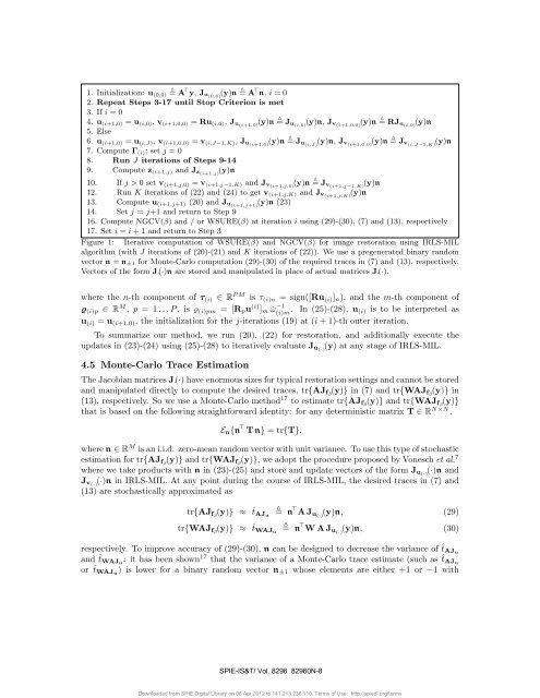
1. Initialization: u △ (0,0) = A ⊤ y, J u(0,0) (y)n = △ A ⊤ n, i =02. Repeat Steps 3-17 until Stop Criterion is met3. If i =04. u (i+1,0) = u (i,0) , v (i+1,0,0) = Ru (i,0) , J u(i+1,0) (y)n = △ J u(i,0) (y)n, J v(i+1,0,0) (y)n = △ RJ u(i,0) (y)n5. Else6. u (i+1,0) = u (i,J) , v (i+1,0,0) = v (i,J−1,K) , J u(i+1,0) (y)n = △ J u(i,J) (y)n, J v(i+1,0,0) (y)n = △ J v(i,J−1,K) (y)n7. Compute Γ (i) ;setj =08. Run J iterations of Steps 9-149. Compute z (i+1,j) and J z(i+1,j) (y)n10. If j>0setv (i+1,j,0) = v (i+1,j−1,K) and J v(i+1,j,0) (y)n = △ J v(i+1,j−1,K) (y)n12. Run K iterations of (22) and (24) to get v (i+1,j,K) and J v(i+1,j,K) (y)n13. Compute u (i+1,j+1) (20) and J u(i+1,j+1) (y)n (23)14. Set j = j+1andreturntoStep916. Compute NGCV(β) and / or WSURE(β) at iteration i using (29)-(30), (7) and (13), respectively17. Set i = i +1andreturntoStep3Figure 1: Iterative computation of WSURE(β) andNGCV(β) for image restoration using IRLS-MILalgorithm (with J iterations of (20)-(21) and K iterations of (22)). We use a pregenerated binary randomvector n = n ±1 for Monte-Carlo computation (29)-(30) of the required traces in (7) and (13), respectively.Vectors of the form J·(·)n are stored and manipulated in place of actual matrices J·(·).where the n-th component of τ (i) ∈ R PM is τ (i)n =sign([Ru (i) ] n ), and the m-th component ofϱ (i)p ∈ R M , p =1...P,isϱ (i)pm =[R p u (i) ] m ˘ω −1(i)m . In (25)-(28), u (i) is to be interpreted asu (i) = u (i+1,0) , the initialization for the j-iterations (19) at (i + 1)-th outer iteration.To summarize our method, we run (20), (22) for restoration, and additionally execute theupdates in (23)-(24) using (25)-(28) to iteratively evaluate J u(·)(y) at any stage of IRLS-MIL.4.5 Monte-Carlo Trace EstimationThe Jacobian matrices J·(·) have enormous sizes for typical restoration settings and cannot be storedand manipulated directly to compute the desired traces, tr{AJ fβ (y)} in (7) and tr{WAJ fβ (y)} in(13), respectively. So we use a Monte-Carlo method 17 to estimate tr{AJ fβ (y)} and tr{WAJ fβ (y)}that is based on the following straightforward identity: for any deterministic matrix T ∈ R N×N ,E n {n ⊤ T n} =tr{T},where n ∈ R M is an i.i.d. zero-mean random vector with unit variance. To use this type of stochasticestimation for tr{AJ fβ (y)} and tr{WAJ fβ (y)}, we adopt the procedure proposed by Vonesch et al. 7where we take products with n in (23)-(25) and store and update vectors of the form J u(·)(·)n andJ v(·)(·)n in IRLS-MIL. At any point during the course of IRLS-MIL, the desired traces in (7) and(13) are stochastically approximated astr{AJ fβ (y)} ≈ ˆt AJu△= n ⊤ AJ u(·)(y)n, (29)tr{WAJ fβ (y)} ≈ ˆt WAJu△= n ⊤ WAJ u(·)(y)n, (30)respectively. To improve accuracy of (29)-(30), n can be designed to decrease the variance of ˆt AJuand ˆt WAJu : it has been shown 17 that the variance of a Monte-Carlo trace estimate (such as ˆt AJuor ˆt WAJu ) is lower for a binary random vector n ±1 whose elements are either +1 or −1 withSPIE-IS&T/ Vol. 8296 82960N-8Downloaded from SPIE Digital Library on 06 Apr 2012 to 141.213.236.110. Terms of Use: http://spiedl.org/terms