MS Word Technical Paper Template

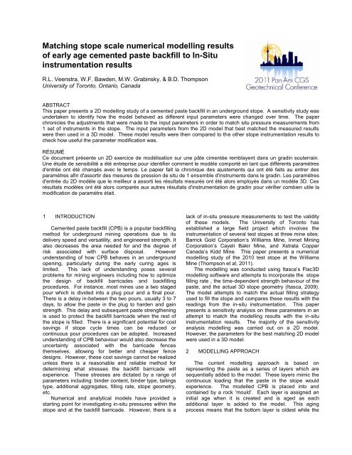
Matching stope scale numerical modelling resultsof early age cemented paste backfill to In-Situinstrumentation resultsR.L. Veenstra, W.F. Bawden, M.W. Grabinsky, & B.D. ThompsonUniversity of Toronto, Ontario, CanadaABSTRACTThis paper presents a 2D modelling study of a cemented paste backfill in an underground stope. A sensitivity study wasundertaken to identify how the model behaved as different input parameters were changed over time. The paperchronicles the adjustments that were made to the input parameters in order to match situ pressure measurements from1 set of instruments in the stope. The input parameters from the 2D model that best matched the measured resultswere then used in a 3D model. These model results were then compared to the other stope instrumentation results tocheck how useful the parameter modification was.RÉSUMÉCe document présente un 2D exercice de modélisation sur une pâte cimentée remblayent dans un gradin souterrain.Une étude de sensibilité a été entreprise pour identifier comment le modèle comporté en tant que différents paramètresd'entrée ont été changés avec le temps. Le papier fait la chronique des ajustements qui ont été faits au entrer desparamètres afin d'assortir des mesures de pression de situ de 1 ensemble d'instruments dans le gradin. Les paramètresd'entrée du 2D modèle que le meilleur a assorti les résultats mesurés ont été alors employés dans un modèle 3D. Cesrésultats modèles ont été alors comparés aux autres résultats d'instrumentation de gradin pour vérifier combien utile lamodification de paramètre était.1 INTRODUCTIONCemented paste backfill (CPB) is a popular backfillingmethod for underground mining operations due to itsdelivery speed and versatility, and engineered strength. Italso decreases the area needed for and the degree ofrisk associated with surface disposal. Howeverunderstanding of how CPB behaves in an undergroundopening, particularly during the early curing ages islimited. This lack of understanding poses severalproblems for mining engineers including how to optimizethe design of backfill barricades and backfillingprocedures. For instance, most mines use a two stagedpour which is divided into a plug pour and a final pour.There is a delay in-between the two pours, usually 3 to 7days, to allow the paste in the plug to harden and gainstrength. This delay and subsequent paste strengtheningis used to protect the backfill barricade when the rest ofthe stope is filled. There is a significant potential for costsavings if stope cycle times can be reduced orcontinuous pour procedures can be adopted. Increasedunderstanding of CPB behaviour would also decrease theuncertainty associated with the barricade fencesthemselves, allowing for better and cheaper fencedesigns. However, these cost savings cannot be realizedunless there is a reasonable and reliable method fordetermining what stresses the backfill barricade willexperience. These stresses are dictated by a range ofparameters including: binder content, binder type, tailingstype, additional aggregates, filling rate, stope geometry,etc.Numerical and analytical models have provided astarting point for investigating in-situ pressures within thestope and at the backfill barricade. However, there is alack of in-situ pressure measurements to test the validityof these models. The University of Toronto hasestablished a large field project which involves theinstrumentation of several test stopes at three mine sites:Barrick Gold Corporation’s Williams Mine, Inmet MiningCorporation’s Cayeli Bakir Mine, and Xstrata CopperCanada’s Kidd Mine. This paper presents a numericalmodelling study of the 2010 test stope at the WilliamsMine (Thompson et al, 2011).The modelling was conducted using Itasca’s Flac3Dmodelling software and attempts to incorporate the stopefilling rate , the time-dependent strength behaviour of thepaste, and the actual 3D stope geometry (Itasca, 2009).The model attempts to match the actual filling strategyused to fill the stope and compares these results with thereadings from the in-situ instrumentation. This paperpresents a sensitivity analysis on these parameters in anattempt to match the modelling results with the in-situinstrumentation results. The majority of the sensitivityanalysis modelling was carried out on a 2D model.However, the parameters for the best matching 2D modelwere used in a 3D model.2 MODELLING APPROACHThe current modelling approach is based onrepresenting the paste as a series of layers which aresequentially added to the model. These layers mimic thecontinuous loading that the paste in the stope wouldexperience. The modelled CPB is placed into andcontained by a rock ‘mould’. Each layer is assigned aninitial age when it is created and is aged as eachadditional layer is added to the model. This agingprocess means that the bottom layer is oldest while the

Cohesion (kPa)Friction Angle (Deg,)uppermost layer is the youngest. Each age has particularinput parameters assigned to it. As the layer ages, thematerial parameters of that layer change so that the timedependentbehaviour of the paste can be mimicked. Inorder to determine the time-dependant input parametersfor the modelling, a laboratory testing program of the CPBwas undertaken and is described in the next section. Themodel was built using a Mohr-Coulomb failure criterion.For a more detailed explanation please refer to Veenstra.et al, 2011.3 LABORATORY TESTINGIn order to determine the time-dependant behaviour ofthe CPB, a laboratory testing program was carried out.This program consisted of direct shear box testing ofdifferent ages of CPB. There were 6 main testing ages:4, 12, 24, 48, 96, and 168 hours (1 week). The testingwas conducted at 4 normal stresses: 50, 100, 250, and400 kPa. This value was chosen as an upper value as itwas at the higher range of observed stresses recorded bythe instrumentation installed in test stopes (Thompson etal 2010). A total of 75 samples for this particular type ofWilliams CPB were tested.Each test had a consolidation and shearingcomponent. The sample was subjected to incrementalnormal loading. Before the next incremental load wasapplied, the sample was allowed to consolidate. After thesample had been loaded to the desired normal stress thesample was sheared.All of the shear box results were analysed todetermine both peak and residual values for cohesionand friction angle. Figure 1 is a graph showing how thecohesion changes with curing time while Figure 2 showshow the friction angle changes with time. These plotsshow how the parameters were changed to simplify themodelling but with keeping the original trends of thelaboratory results intact.The tested paste has no or very low cohesion when itis fresh. The cohesion then increases steadily for the first96 hours of curing, after which the rate of cohesion gainplateaus at around 33 kPa. However, the friction angle ofthe tested paste shows remarkable little change withcuring time, with the friction angle values varying from 35to 41 over 168 hours. These curves were smoothed andthen were used as input parameters in the model.3530252015105Cohesion95% Conf. Int.Model InputsEND OF POUR00 10 20 30 40 50 60 70 80 90 100Cure Time (hrs)Figure 1. Cohesion versus Cure Time45403530252015END OF POURFriction Angle1095% Conf. Int5Model Inputs00 10 20 30 40 50 60 70 80 90 100Cure Tume (hrs)Figure 2. Friction Angle versus Cure Time4 MODELLING SPECIFICS FOR WILLIAMS 2010TEST STOPEFigure 3a shows a 3D cavity monitoring survey (CMS)taken of the Williams 2010 test stope. Figure 3b showsthe 2D model geometry, and Figure 3c shows the 3Dmodel geometry of the Flac3D model. Note that some ofthe dimensions were changed to be divisible by 0.2 m,which was the model zone size. All of the followingdimensions are for the model geometry and not the actualstope geometry. Please note that the dimensions shownin Figure 3b and 3c are for the paste contained within therock mould and not for the rock mould that is shown inthe figure. The 3D stope model was 6 m wide and was18.8 m along strike length, while the body of the stopewas approximately 50 m high and dipped at 65 degrees.The access drift was approximately 4.6 m high by 4.4 mwide, with the barricade being 9.2 m from the stope browand located in the approximate centre of the stope strikelength. It should be noted that this stope was a hangingwall access stope. The 2D model cuts a section throughthe body of the stope looking along the strike length. Thetotal pour time was approximately 68 hours. The modelwas constructed with 0.2 m zones. This size was acompromise between the filling rate and the amount ofzones within the model. This meant that the model wasrun at 2 hour increments.There were three sets of instruments installed in thestope. Two sets were centred around cages, while thethird set was installed on the barricade fence. Figure 4ashows an instrumented cage: there are 3 orthogonallyarranged total earth pressure cells (TEPCs) and apiezometer (PZ) in each cage. Figure 4b shows anexample of the instrument panel that was installed on thefence and contains 1 TEPC and one PZ. Two suchpanels were installed along the centreline of the fence.Figure 4c shows the two instrumented cages installedinto the stope. Note that one of the cages is in theapproximate centre of the stope body while the othercage is located into the drift. Figure 5 is a schematicdetailing the locations of the instruments within the stope.Note that for the 2D modelling only the results from Cage2 were used for matching purposes, with the horizontalstress direction being perpendicular to the strike length(X-Direction in the models)

a)Figure 4.a) Instrumented cage (from Thompson et al,2010), b) Installed Instrument Cages, c) FenceInstrumentationc)b) c)Figure 3.a) Stope CMS (from Thompson et al 2010) b) 2DModel Geometry c) 3D Model GeometryFigure 5. Schematic of Instrument Installation5 MODELLING SPECIFICS FOR WILLIAMS 2010TEST STOPEa) b)This section presents the modelling results generatedfrom the baseline input parameters. Figures 2a and bshow how the baseline input parameters change overtime. Figure 6 shows the results from the baselinemodel, with part a) showing the modelled and measuredvertical and horizontal stresses versus time. Figure 6bpresents the same data but concentrates on the first 30hours of the pour. Figure 6c compares the ratio ofhorizontal to vertical stress for both the modelled andmeasured results. The three graph setup will be used for

Stress (kPa)Stress (kPa)σh/σvFriction Angle (deg.)Friction Angle (deg.)Friction Angle (deg.)Friction Angle (deg.)Friction Angle (deg.)presenting the 2D modelling results in the remainder ofthis paper. Figures 6a and b both have a hydrostaticstress line representing the vertical stress. This wasdetermined by multiplying the height of the paste by theunit weight of the material.140120100806040200a1008060ZInst. ZXInst. X0 10 20 30 40 50 60 70Pour Time (hrs)as quickly as the test sample. This means that the instopeCPB, at least during early curing ages, is eitherundrained or partially drained, thus the frictional term willvary from zero in early age paste to some value in olderpaste.In this paper the approach for modelling thisbehaviour was to change the friction angle instead ofincorporating PWP pressure into the model. This wouldstill cause the frictional component to increase from 0 inthe early age paste to the laboratory friction values ofolder paste. A sensitivity analysis for friction angle ispresented in the next section (6). Cohesion, according tothe equation, should not be affected by PWP. However,it is important to know what effect cohesion has on themodel. Therefore, a sensitivity analysis for cohesion ispresented in Section 7.bc4020010.90.80.70.60.50.40.30.20.10ZInst. ZXInst. X0 5 10 15 20 25 30Pour Time (hrs)BaselineInst.0 10 20 30 40 50 60 70Pour Time (hrs)Figure 6. Baseline Model a) Modelled Stresses b)Closeup of ‘a’ c) Horizontal to Vertical Stress RatioFigure 6b highlights two differences between theinstrumentation and modelled results. The first differenceis that the modelled vertical stress rises more rapidly thanthe measured vertical stress. Explanations for this includea difference in filling rate or density; however thisdiscrepancy will not be examined further in this paper.The second difference is that the measured data trackstogether for the first 2 to 4 hours and then starts toseparate. Please note that the time axis is pour time andnot cure time. However, the modelled data separatesright from the beginning and never tracks. The observedtracking indicates that the vertical and the horizontalstress are equal or hydrostatic. This also indicates that,during this early age of curing, the CPB has very littleshear strength. The Mohr-Coulomb shear stressequation is given below:6 SENSITIVITY ANALYSIS OF FRICTION ANGLESix different scenarios for frictional change wereexamined and are summarized in Figures 7a-e. The first(a) assumes constant friction at 0°, 20°, 40°, and 60° offriction. The second (b) assumes a constant increase offriction from 0° to 20° over the first 96 hours of curingtime, with the same scenario repeated for 40° and 60°.The third (c) assumes that there is no frictional increaseover the first 4 hours of curing and then repeats thepattern over the remaining 96 hours. A delay of 4 hourswas used as this was the maximum length of time,observed in Figure 6b, where the measured vertical andhorizontal stresses were hydrostatic. The fourth (d)scenario assumes no frictional increase over the first 4hours, with increases then taking place over the next 6hours, followed by constant friction values. The finalscenario (e) assumes no frictional increase for 4 hours,followed by an instantaneous frictional increase, followedby constant friction values for the remainder of the 96hours.a7060504030201000 20 40 60 80 100Cure Time (hrs)706050b7060504030201000 20 40 60 80 100Cure Time (hrs)706050c7060504030201000 20 40 60 80 100Cure Time (hrs)[1]403020403020where τ is shear stress, c is cohesion, σ n is the appliednormal stress, μ is the pore water pressure (PWP), and υis the friction angle. If the PWP is equal to the normalstress, the frictional component of the equation is zerowhereas, if the PWP is zero, the frictional component isat a maximum value.In the case of the laboratory testing presented inSection 3, the tests were run allowing free drainage andwere allowed to consolidate before the sample wassheared. This means that the testing was carried out withgreatly reduced PWP meaning that frictional componentof the above equation would be some value above zero.However, it is unlikely that the in-stope CPB would drain100d0 20Cure40Time (hrs)60 80 100100e0 20Cure40Time (hrs)60 80 100Figure 7.a) Constant Friction b) Ramped Friction c)Delayed Ramped Friction d) Delayed Steeply RampedFriction e) Delayed Instantaneous FrictionFigures 8a-b show the results of the scenariospresented in figure 7a. This figure shows that the frictionhas a large impact on the shape of the curves, which isobserved in the difference between the 0° friction and 20°friction curves. However there is less impact at higherfriction angles as observed by the limited differencesbetween the 40° and 60° friction curves. Please note that

σh/σvStress (kPa)Stress (kPa)σh/σvσh/σvStress (kPa)Stress (kPa)Stress (kPa)Stress (kPa)the modelled horizontal and vertical stresses in the 0°friction curves track. This is seen in the Figure 7c).c350300250200150100500a150b125100755025010.90.80.70.60.50.40.30.20.100 10 20 30 40 50 60 70Pour Time (hrs)0° Z0° X20° Z20° X40° Z40° X60° Z60° XInst. ZInst. X0° 20° 40°60° Inst.0° Z 0° X20° Z 20° X40° Z 40° X60° Z 60° XInst. ZInst. X0 5 10 15 20 25 30Pour Time (hrs)0 10 20 30 40 50 60 70Pour Time (hrs)Figure 8. Modelling Results from Figure 7a) ParametersFigures 9a-b show the results of the scenariospresented in figure 7b. This figure shows the impact thatfrictional variation has on the model. The first effect is thestresses are much higher than in Figure 8. However, thevertical and horizontal stresses are tracking as is shownin c).a150b35030025020015010050012510075502500 5 10 15 20 25 30Pour Time (hrs)10.90.80.70.60.50.40.320° Z20° X40° Z40° X60° Z60° XInst. ZInst. X0 10 20 30 40 50 60 70Pour Time (hrs)20° Z20° X40° Z40° X60° Z60° XInst. ZInst. X0.220° Inst.0.140° 60°00 10 20 30 40 50 60 70cPour Time (hrs)Figure 9. Modelling Results from Figure 7b) Parametersabc350300250200150100500150125100755025010.90.80.70.60.50.40.30.20.1020° Friction-Z 20° Friction-X40° Friction-Z 40° Friction-X60° Friction-Z 60° Friction-XInst. X0 10 20 30 40 50 60 7020° Friction-Z20° Friction-X40° Friction-Z40° Friction-X60° Friction-Z60° Friction-XInst. XInst. ZInst. ZPour Time (hrs)0 5 10 15 20 25 30Pour Time (hrs)20° Friction 40° Friction60° Friction Inst.0 10 20 30 40 50 60 70Pour Time (hrs)Figure 10. Modelling Results from Figure 7c) ParametersThe previous figures (8, 9, and 10) all show stressesthat are much higher than the measured stresses. Thenext scenario was designed to examine how aninstantaneous increase in frictional strength woulddecrease the stresses in the CPB. Figures 11a-b showthe results of the scenarios presented in Figure 7d. Thisscenario has significantly dropped the CPB stressesthough they are still too high when compared to themeasured values. However the horizontal to verticalstress ratio in 11c) is a good match to the measuredstress ratioHowever, the stresses observed in Figure 11 are stillhigh so the next scenario incorporated an instantaneousgain of friction. Figures 12a-b show the results of thescenario presented in Figure 7e. The use ofinstantaneous friction successfully lowers the modelledstresses by 20 kPa and is much closer to the measuredvalues. This is particularly true of the 40° friction curve,which is the close to the laboratory friction value of 38°.However, the difference in the behaviour between the 20°and the other friction angle curves was unexpected.There are some relationships observed in themodelled data. The first is that friction has a large impacton the behaviour of the modelled paste, particularly atlower friction angles. The second is how fast the modelrequires the friction angle to rise from zero to thelaboratory values. This indicates, using the processdescribed in Section 5, the PWP in the in-stope CPBdissipates relatively quickly.Figures 10a-b show the results of the scenariospresented in figure 7c. This scenario was designed tosee how delaying the onset of friction would change thestresses. The modelled stresses are higher than whatwas seen in Figure 9. However, the ratios observed in10c) are similar to in 9c).

σh/σvσh/σvStress (kPa)Stress (kPa)Stress (kPa)Stress (kPa)σh/σvStress (kPa)Stress (kPa)Cohesion (kPa)Cohesion (kPa)16014080708070a150b120100806040200125100755025Inst. ZInst. X00 5 10 15 20 25 30Pour Time (hrs)10.90.80.70.60.50.40.30.20.120° Z 20° X40° Z 40° X60° Z 60° XInst. Z0 10 20 30 40 50 60 70Pour Time (hrs)20° Z 20° X40° Z 40° X60° Z 60° X20° 40°60° Inst.Inst. X00 10 20 30 40 50 60 70cPour Time (hrs)Figure 11. Modelling Results from Figure 7d) Parametersc160140120100806040200a150b125100755025010.90.80.70.60.50.40.30.20.1020° Z 20° X 40° Z 40° X60° Z 60° X Inst. Z Inst. X0 10 20 30 40 50 60 70Pour Time (hrs)20° Z20° X40° Z40° X60° Z60° XInst. ZInst. X0 5 10 15 20 25 30Pour Time (hrs)20° 40°60° Inst.0 10 20 30 40 50 60 70Pour Time (hrs)Figure 12. Modelling Results from Figure 7e) Parameters7 SENSITIVITY ANALYSIS OF COHESIONThe two scenarios were used to examine cohesionare summarized in Figures 13a and b. Both scenariosassume the frictional properties of the 40° line in Figure7e. The first scenario assumes constant cohesion overthe first 96 hours of curing at 0 kPa, 17 kPa, 35 kPa, and70 kPa. The second scenario assumes an increase incohesion from 0 kPa to the values mentioned above, overthe first 96 hours of curing.a60504030201000 20 40 60 80 100Cure Time (hrs)b60504030201000 20 40 60 80 100Cure Time (hrs)Figure 13. a) Continuous and b) Ramped CohesionFigures 14a-c show the modelling results based onthe scenario shown in Figure 13a). The main trend in thisfigure is that changing the cohesion, except for thechange from 0 kPa to 17 kPa, has little impact on theoverall strength of the paste. However, when this figureis compared to the 40° line of Figure 12a, the maindifference is the observed stress increases due to theinstantaneous cohesion at the start of curing. However,this instantaneous cohesion has a negative impact on thehorizontal to vertical stress ratio. The next scenario (13b)examines the influence of this early cohesion and themodelling results are shown in Figures 15a-c.c180160140120100806040200a160b14012010080604020010.90.80.70.60.50.40.30.20.100 kPa Z 0 kPa X 17 kPa Z 17 kPa X35 kPa Z 35 kPa X 70 kPa Z 70 kPa XInst. ZInst. X0 10 20 30 40 50 60 70Pour Time (hrs)0 kPa Z0 kPa X17 kPa Z17 kPa X35 kPa Z35 kPa X70 kPa Z70 kPa XInst. ZInst. X0 5 10 15 20 25 30Pour Time (hrs)0 kPa Inst. 17 kPa35 kPa 70 kPa0 10 20 30 40 50 60 70Pour Time (hrs)Figure 14. Modelling Results from Figure 13a)ParametersThere is very little difference between Figure 15 andFigure 12. This implies that the ramping up of cohesion,as exhibited in the laboratory testing in Figure 2, has verylittle impact on the strength of this CPB. These resultsindicate that cohesion has minimal effect on the strengthof the paste, and only if it is applied early during curing. Itseems that the behaviour of the paste is driven mainly byfriction angle.

Stress (kPa)Stress (kPa)σh/σvStress (kPa)Stress (kPa)(σh/σv)Stress (kPa)c180160140120100806040200a160b14012010080604020010.90.80.70.60.50.40.30.20.1017 kPa Z 17 kPa X 35 kPa Z 35 kPa X70 kPa Z 70 kPa X Inst. Z Inst. X0 10 20 30 40 50 60 70Pour Time (hrs)17 kPa Z17 kPa X35 kPa Z35 kPa X70 kPa Z70 kPa XInst. ZInst. X0 5 10 15 20 25 30Pour Time (hrs)17 kPa Inst.35 kPa 70 kPa0 10 20 30 40 50 60 70Pour Time (hrs)Figure 15. Modelling Results from Figure 13b)Parameters8 3D RESULTS BASED ON INPUTS FROM 2DMODELLINGThe 3D model was run using the same parameters thatwere used in the cohesion sensitivity analysis. This is apartial check on the 2D results. The 2D model could onlybe compared to one of the instrumented cages sorunning the 3D model will check the modelling resultsagainst the other instrumentation. The results are shownin Figures 16a-d. These results show that 3D modellingresults agree well with the measured data, and are muchcloser than the original iteration of the model presented inVeenstra et al, 2011. The modelled and measuredhorizontal stresses match more closely; in particular, thedifference between the measured and modelled fencepressures has been reduced.14012010080604020C1-ZC2-ZC1Z Inst.C2Z Inst.00 10 20 30 40 50 60 70aPour Time (hrs)10080604020C1-X C1-Y C2X Inst.C2Y Inst. C2-X C2-YC1X InstC1Y Inst00 10 20 30 40 50 60 70bPour Time (hrs)10.90.80.70.60.50.40.30.20.15045403530252015FC1-X FC1-Y C1-X C1-YFC2-X FC2-Y C2-X C2-Y00 10 20 30 40 50 60 70cPour Time (hrs)10F1 - low F2 - high5F1 - Inst. F2 - Inst.00 10 20 30 40 50 60 70dPour Time (hrs)Figure 16. 3D Model using the Parameters from the BestMatched 2D Model a) Vertical Stresses b) HorizontalStresses c) Horizontal to Vertical Stress Ratio d) FencePressures9 SUMMARYThis paper presents the modelling results of asensitivity analysis performed on CPB laboratory testingresults. The goal was to match the modelling data to themeasured field data from in-situ instrumentation in thestope. In order to do this the frictional component of theMohr-Coulomb equation [1] was examined. In order tomatch the hydrostatic stress tracking measured by theinstrumentation it was necessary to decrease thisfrictional component. The rationale behind this was theidea that the CPB is either undrained or partiallyundrained during early curing ages. This means that thePWP was equal or only slightly less than applied normalstresses resulting in a decreased frictional component ofthe equation [1].The frictional sensitivity study found that the modelledCPB is very dependent on the friction angle. It also foundthat the model required a very rapid increase in frictionangle in order to match the measured data. This impliesthat the PWP pressure in the CPB dissipates relativelyquickly. The scenario where there was no frictionalincrease for 4 hours, followed by an instantaneousfrictional increase to 40°, after which the friction anglewas constant provided the closest match between themodelling and measured results. A more detailedexamination of this early curing age frictional behaviourmay provide a better match. Additionally, the actual riseratein the stope needs to be better qualified as thecurrently modelled rate seems faster than the actual rate.An examination of the effects of cohesion showed thatcohesion, unless applied early during the curing period,has limited effect on the strength of the CPB. It alsofound that increasing the amount of cohesion, as long asthere was cohesion, produced minimal differences in thestrength of the modelled CPB.

10 ACKNOWLEDGMENTSMatt Pierce and David Sainsbury of Itasca Consulting,Summer Students Robin Malik and Michelle Moore,Research Associate Dragana Simon, and Brian Zurawski.of WOC.11 REFERENCESItasca Consulting Group, Inc. 2009. FLAC3D: FastLagrangian Analysis of Continua in 3 Dimensions.Version 4.0. ICG, Minneapolis MN, USA.Thompson, B.D, Grabinksy, M.W., Bawden, W.F. 2010.Field Report of Williams Mine Paste Project 2010:9500 L70-5. University of Toronto, Toronto, ON,Canada.Thompson, B.D, Grabinsky, M.W, Veenstra, R.L., andBawden, W.F. 2011. In situ pressures in cementedpaste backfill – a review of field work from threemines. Paste 2011, AC, Perth, Australia. 491-504.Veenstra, R.L., W.F. Bawden, M.W. Granbinsky, B.D.Thompson. 2011 An Approach to Stope ScaleNumerical Modelling of Early Age Cemented PasteBackfill. 45 th US Rock Mechanics / GeomechanicsSymposium, ARMA, San Francisco, CA, USA.(submitted)