Lecture 2: Controllability of nonlinear systems

DISC Systems and Control Theory of Nonlinear Systems 1Lecture 2:Controllability of nonlinear systemsNonlinear Dynamical Control Systems, Chapter 3See www.math.rug.nl/˜arjan (under teaching) for info on courseschedule and homework sets.Take-Home Exam I on homepage on March 16.

DISC Systems and Control Theory of Nonlinear Systems 2Recall: Kinematic model of the unicycleẋ 1 = u 1 cosx 3ẋ 2 = u 1 sinx 3ẋ 3 = u 2written as a system with two input vector fields and zero driftvector field⎡ ⎤ ⎡ ⎤cosx 3 0ẋ = ⎢⎣sin x 3⎥⎦ u 1 + ⎢⎣0⎥⎦ u 20 1The Lie bracket of the two input vector fields is given as⎡ ⎤ ⎡ ⎤ ⎡ ⎤0 0 − sinx 3 0 sinx 3− ⎢⎣0 0 cosx 3⎥ ⎢⎦ ⎣0⎥⎦ = ⎢⎣− cosx 3⎥⎦0 0 0 1 0

DISC Systems and Control Theory of Nonlinear Systems 3which is a vector field that is independent from the two inputvector fields.Claim: This new independent direction guarantees controllabilityof the unicycle system.Interpretation of the Lie bracket:Proposition 1 Let X, Y be two vector fields such that[X, Y ] = 0Then the solution flows of the vector fields are commuting.In fact, we may find local coordinates x 1 , . . .,x n such thatX = ∂∂x 1,Y = ∂∂x 2Thus, the Lie bracket [X, Y ] characterizes the amount ofnon-commutativity of the vector fields X, Y .

DISC Systems and Control Theory of Nonlinear Systems 4In fact, let the control strategy u = col(u 1 , u 2 ) be defined by⎧(1, 0), t ∈ [0, ε), ε > 0⎪⎨ (0, 1), t ∈ [ε, 2ε)u(t) =(−1, 0), t ∈ [2ε, 3ε)⎪⎩(0, −1), t ∈ [3ε, 4ε),Then the motion of the system is described byx(4ε) = x 0 + ε 2 [g 1 , g 2 ](x 0 ) + O(ε 3 ).which indicates controllability, since [g 1 , g 2 ] is everywhereindependent from g 1 , g 2 .This formula holds in general.This is enough for systems with two inputs and three statevariables, but what can we do if the dimension of the state is > 3?

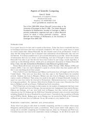
DISC Systems and Control Theory of Nonlinear Systems 5Answer: consider higher-order Lie brackets.y r■θ▼ϕx rExample 2 Consider the cart with fixed rear axis⎡ ⎤ ⎡ ⎤ ⎡ ⎤x 1 cos(ϕ + θ) 0dx 2sin(ϕ + θ)0=udt ⎢⎣ ϕ ⎥ ⎢⎦ ⎣ sinθ ⎥ 1 +⎢⎦ ⎣ 0 ⎥⎦θ 01with u 1 the driving input, and u 2 the steering input.u 2

DISC Systems and Control Theory of Nonlinear Systems 6Defineg 1 (x) =⎡ ⎤cos(x 3 + x 4 )sin(x 3 + x 4 ), g⎢⎣ sin(x 4 ) ⎥ 2 (x) =⎦}0{{ }Drive⎡ ⎤00.⎢⎣ 0 ⎥⎦1} {{ }Steer

DISC Systems and Control Theory of Nonlinear Systems 7Compute[Steer, Drive] = ∂g 1∂x g 2 − ∂g 2∂x g 1⎡0 0 − sin(x 3 + x 4 ) − sin(x 3 + x 4 )0 0 cos(x 3 + x 4 ) cos(x 3 + x 4 )=⎢⎣ 0 0 0 cos(x 4 )0 0 0 0⎡⎤− sin(x 3 + x 4 )cos(x 3 + x 4 )==: Wriggle.⎢⎣ cos(x 4 ) ⎥⎦0⎤⎡⎥⎢⎦⎣0001⎤⎥⎦− 0

DISC Systems and Control Theory of Nonlinear Systems 8Another independent direction is obtained by the third-order Liebracket⎡ ⎤− sin(x 3 )cos(x 3 )[Wriggle, Drive] ==: Slide.⎢⎣ 0 ⎥⎦0This shows that you can manoeuver your car into any parking lotby applying controls corresponding to the ‘Slide’ direction, i.e., byapplying the control sequence {Wriggle, Drive, −Wriggle, −Drive}.

DISC Systems and Control Theory of Nonlinear Systems 9What to do with the drift vector field ?The systemẋ = f(x) + g(x)ucan be considered as a special case ofẋ = g 1 (x)u 1 + g 2 (x)u 2 ,with u 1 = 1. This means that care has to be taken with respect tobrackets involving f:[f, g], [g, [f, g]], [f, [f, g]], . . .

DISC Systems and Control Theory of Nonlinear Systems 10Example 3 Consider the system on R 2ẋ 1 = x 2 2ẋ 2 = u.Compute the Lie brackets of the vector fields⎡ ⎤ ⎡ ⎤f(x) =⎣ x2 20⎦, g(x) =⎣ 0 1⎦ ,yielding⎡⎤⎡⎤[f, g](x) =⎣ −2x 20⎦ , [[f, g], g](x) =⎣ 2 0⎦.Clearly, we have obtained two independent directions. However,since x 2 2 ≥ 0, the x 1 -coordinate is always non-decreasing. Hence,the system is not really controllable.

DISC Systems and Control Theory of Nonlinear Systems 11A weaker form of controllability: local accessibilityLet V be a neighborhood of x 0 , then R V (x 0 , t 1 ) denotes thereachable set from x 0 at time t 1 ≥ 0, following the trajectorieswhich remain in the neighborhood V of x 0 for t ≤ t 1 , i.e., all pointsx 1 for which there exists an input u(·) such that the evolution ofthe system for x(0) = x 0 satisfies x(t) ∈ V, 0 ≤ t ≤ t 1 , and x(t 1 ) = x 1 .Furthermore, letR V t 1(x 0 ) = ⋃R V (x 0 , τ).τ≤t 1Definition 4 (Local accessibility) A system is said to be locallyaccessible from x 0 if R V t 1(x 0 ) contains a non-empty open subset ofX for all non-empty neighborhoods V of x 0 and all t 1 > 0. If thelatter holds for all x 0 ∈ X then the system is called locallyaccessible.

DISC Systems and Control Theory of Nonlinear Systems 12Definition 5 (Accessibility algebra) Consider the systemẋ = f(x) + g 1 (x)u 1 + · · · + g m (x)u mThe accessibility algebra C are the linear combinations ofrepeated Lie brackets of the form[X k , [X k−1 , [· · · , [X 2 , X 1 ] · · ·]]], k = 1, 2, . . .,where X i , is a vector field in the set {f, g 1 , . . .,g m }.This linear space is a Lie algebra under the Lie bracket.Definition 6 The accessibility distribution C is the distributiongenerated by the accessibility algebra C:C(x) = span{X(x) | X vector field in C}, x ∈ X

DISC Systems and Control Theory of Nonlinear Systems 13Intermezzo: Distributions on manifoldsA distribution D on a manifold X is specified by a subspaceD(x) ⊂ T x Xfor all x ∈ X.Let X 1 , X 2 , . . .,X k be vector fields on X. ThenD(x) = span(X 1 (x), X 2 (x), . . .,X k (x)).defines a distribution.A distribution D is called involutive if, whenever f, g ∈ D, also[f, g] ∈ D.The distribution D is called constant-dimensional whenever thedimension of D(x) is constant.

DISC Systems and Control Theory of Nonlinear Systems 14Example 7 Let X = R 3 and D = span(f 1 , f 2 ), wheref 1 (x) =⎡⎢⎣2x 210⎤⎥⎦ , f 2(x) =⎡⎢⎣⎤10 ⎥⎦ .x 2Since f 1 and f 2 are linearly independent, we have thatdim(D(x)) = 2, for all x. Furthermore, we have[f 1 , f 2 ](x) = ∂f 2∂x (x)f 1(x) − ∂f 1∂x (x)f 2(x) =⎡⎢⎣100⎤⎥⎦ .

DISC Systems and Control Theory of Nonlinear Systems 15[f 1 , f 2 ] ∈ D if and only if rank(f 1 (x), f 2 (x), [f 1 , f 2 ](x)) = 2, for all x.However,rank(f 1 (x), f 2 (x), [f 1 , f 2 ](x)) = rankfor all x. Hence, D is not involutive.⎡⎢⎣2x 2 1 01 0 00 x 2 1⎤⎥⎦ = 3,

DISC Systems and Control Theory of Nonlinear Systems 16Let D be a nonsingular distribution on X, generated by theindependent vector fields f 1 , . . .,f r . Then D is said to be integrableif for each x 0 ∈ X, there exists a neighborhood N of x 0 and n − rreal-valued independent functions h 1 (x), . . .,h n−r (x) defined on N,such that h 1 (x), . . .,h n−r (x) satisfy the partial differential equationsfor all indices i = 1, . . .,r, j = 1, . . .,n − r.Frobenius’ theorem∂h j∂x (x)f i(x) = 0, (1)A constant-dimensional distribution is integrable if and only if it isinvolutive.The necessity of involutivity for complete integrability is easilyseen. Indeed, suppose that (1) is satisfied. This is the same asL fi h j = 0

DISC Systems and Control Theory of Nonlinear Systems 17It follows thatL [fi ,f k ]h j = L fi L fk h j − L fk L fi h j = 0Since the functions h 1 (x), . . .,h n−r (x) are independent, this impliesthat the Lie brackets [f i , f k ] are (pointwise) linear combinations ofthe vector fields f 1 , . . .,f r , and are thus contained in thedistribution D.A geometric description of Frobenius’ theorem is as follows. Letthe independent functions h 1 (x), . . .,h n−r (x) satisfy (1). Then theirlevel sets, i.e., all sets of the form{x | h 1 (x) = c 1 , . . .,h n−r (x) = c n−r }for arbitrary constants c 1 , . . .,c n−r , are well-defined r-dimensionalsubmanifolds of X, to which all the vector fields f 1 , . . .,f r aretangent, and, as a consequence, also all their Lie brackets aretangent.

DISC Systems and Control Theory of Nonlinear Systems 18Example 8 Consider the following set of partial differentialequations0 = x 1∂φ∂x 1+ x 2∂φ∂x 2+ x 3∂φ∂x 30 = ∂φ∂x 3Define the vector fieldsf 1 (x) =⎡⎢⎣⎤ ⎡x 1x 2⎥⎦ , f 2(x) = ⎢⎣x 3001⎤⎥⎦ .It is checked that D := span(f 1 , f 2 ) has constant dimension = 2 onthe set X = {x ∈ R 3 | x 2 1 + x 2 2 ≠ 0} (that is, R 3 excluding the x 3 -axis),and is involutive. Thus, by Frobenius’ theorem, D is integrable.

DISC Systems and Control Theory of Nonlinear Systems 19Consequently, for each x 0 ∈ X, there exists a neighborhood N of x 0and a real-valued function φ(x) with dφ(x) ≠ 0 that satisfies thegiven set of partial differential equations. In fact, φ(x) = lnx 1 − lnx 2is a (global) solution.Note that the solution is not unique. In particular, φ(x) = tan −1 x 2x 1isalso a global solution.

DISC Systems and Control Theory of Nonlinear Systems 20By construction, the accessibility distribution C is involutive.Theorem 9 (Local accessibility) A sufficient condition for thesystem to be locally accessible from x ∈ X isdimC(x) = n (2)If this holds for all x ∈ X then the system is locally accessible.Conversely, if the system is locally accessible then (2) holds for allx in an open and dense subset of X.We call (2) the accessibility rank condition at x.

DISC Systems and Control Theory of Nonlinear Systems 21Key idea of the proofConsider the systemẋ = f(x) + g 1 (x)u 1 + . . .g m (x)u mand its generated system vector fieldsF = {X | ∃u 1 , . . .,u m such that X(x) = f(x) + g 1 (x)u 1 + . . .g m (x)u m }Then for every k ≤ n there exists a submanifold N k around x 0 ofdimension k given asN k = {x | x = X t kk ◦ Xt k−1k−1 ◦ · · · ◦ Xt 11 (x 0), 0 ≤ σ i < t i < τ i }with X i ∈ F. Indeed, suppose for a certain k < n we cannotconstruct N k+1 . This means that all system vector fields X ∈ F aretangent to N k , and hence all vector fields f, g 1 , . . .,g m . This alsomeans that all Lie brackets of these vector fields are tangent toN k , and thus dim C(x) ≤ k, which is a contradiction.

DISC Systems and Control Theory of Nonlinear Systems 22If there is no drift vector field then we obtain real controllability:Theorem 10 Considerẋ = g 1 (x)u 1 + g 2 (x)u 2 + . . . + g m (x)u mIf dimC(x) = n for all x ∈ X then the system is controllable.Consider the map(t 1 , . . .,t n ) → X t nn ◦ X t n−1n−1 ◦ · · · ◦ Xt 11 (x 0), 0 ≤ σ i < t i < τ ihaving image N n , which is an n-dimensional open part of X.Now let s 1 , . . .,s n be such that 0 ≤ σ i < s i < τ i . Then the map(t 1 , . . .,t n ) → (−X 1 ) s 1◦(−X 2 ) s 2◦· · ·◦(−X n ) s n◦X t nn ◦X t n−1n−1 ◦· · ·◦Xt 11 (x 0), 0 ≤ σ i < t i < τ ihas an image which is an open neighborhood of x 0 . Thus thereachable set R(x 0 ) from x 0 contains an open neighborhood of x 0 .

DISC Systems and Control Theory of Nonlinear Systems 23Suppose now that the reachable set is smaller than X. Then takeany point on the boundary of the reachable set R(x 0 ). Then the setof points reachable from this point is again open. Contradiction.Thus the unicycle and the cart are indeed controllable.Note that the actual construction of the input functions whichsteers the system from x 0 to x 1 has not been addressed.

DISC Systems and Control Theory of Nonlinear Systems 24Sometimes local accessibility is heavily depending on the flow ofthe drift vector field; consider for example the systemẋ 1 = 1ẋ 2 = uThis system is locally accessible, but of course very far fromcontrollability. In order to improve the situation we look at astronger form of accessibility: local strong accessibilityA system is locally strongly accessible from x 0 if for anyneighborhood V of x 0 the set R V (x 0 , t 1 ) contains a non-empty setfor any t 1 > 0 sufficiently small. If the latter holds for all x ∈ X thenthe system is called locally strongly accessible.(The example given above is not locally strongly accessible.)

DISC Systems and Control Theory of Nonlinear Systems 25Define C 0 as the smallest algebra which contains g 1 , . . .,g m andsatisfies [f, w] ∈ C 0 for all w ∈ C 0 . Define the correspondinginvolutive distributionC 0 (x) := span{X(x) | X vector field in C 0 }.We refer to C 0 and C 0 as the strong accessibility algebra and thestrong accessibility distribution, respectively.

DISC Systems and Control Theory of Nonlinear Systems 26Notice that the strong accessibility algebra C 0 does not contain thedrift vector field f).Theorem 11 (Strong accessibility) A sufficient condition for thesystem to be locally strongly accessible from x isdimC 0 (x) = nFurthermore, the system is locally strongly accessible if this holdsfor all x. Conversely, if the system is locally strongly accessiblethen it holds for all x in an open and dense subset of X.The system given before:ẋ 1 = x 2 2ẋ 2 = u.is not only locally accessible, but also locally strongly accessible,since g(x) and [[f, g], g](x) are everywhere independent.

DISC Systems and Control Theory of Nonlinear Systems 27Let us apply the theory developed above to a linear systemẋ = Ax +m∑b i u i , x ∈ R n ,i=1where b 1 , . . .,b m are the columns of the input matrix B.Clearly, the Lie brackets of the constant input vector fields given bythe input vectors b 1 , . . .,b m are all zero, i.e.,[b i , b j ] = 0, for all i, j = 1, . . .,m.Furthermore, the Lie bracket of the linear drift vector field Ax withan input vector field b i yields the constant vector field[Ax, b i ] = −Ab i .The Lie brackets of Ab i with Ab j or b j are again all zero, while[Ax, −Ab i ] = A 2 b i .

DISC Systems and Control Theory of Nonlinear Systems 28Hence we conclude that C is spanned by all constant vector fieldsb i , Ab i , A 2 b i , . . ., i ∈ m, together with the linear drift vector field Ax,i.e.,C = {Ax, b i , Ab i , A 2 b i . . .,A n−1 b i , i = 1, . . .,m}.whileC 0 = columns of (B, AB, A 2 B . . .,A n−1 B)We see that for linear systems the rank condition for strongaccessibility coincides with the Kalman rank condition forcontrollability. Hence, if we would not have known anything specialabout linear systems, then at least a linear system which satisfiesthe Kalman rank condition is locally strongly accessible.

DISC Systems and Control Theory of Nonlinear Systems 29Example 12 (Actuated rotating rigid body)Consider⎡ ⎤ ⎡ ⎤ ⎡ ⎤ ⎡ ⎤˙ω 1 A 1 ω 2 ω 3 α 1 0⎢⎣ ˙ω 2⎥⎦ = ⎢⎣A 2 ω 3 ω 1⎥⎦ + ⎢⎣ 0 ⎥⎦ u 1 + ⎢⎣α 2⎥⎦ u 2˙ω 3 A 3 ω 1 ω 2 0 0with α 1 ≠ 0, α 2 ≠ 0. Here the constants A 1 , A 2 , A 3 are determined bythe moments of inertia a 1 , a 2 , a 3 . Compute⎡ ⎤0[g 1 , f](ω) = ⎢⎣α 1 A 2 ω 3⎥⎦α 1 A 3 ω 2[g 2 , f](ω) =⎡ ⎤α 2 A 1 ω 3⎢⎣ 0 ⎥⎦α 2 A 3 ω 1

DISC Systems and Control Theory of Nonlinear Systems 30On the other hand⎡ ⎤0[g 2 , [g 1 , f]] = ⎢⎣ 0 ⎥⎦α 1 α 2 A 3Thus the system is locally strongly accessible ifA 3 ≠ 0which is equivalent to a 1 ≠ a 2 .In fact, this is the if and only if condition. Indeed, if A 3 = 0 then˙ω 3 = 0, showing that the system is not locally strongly accessible.Remark 13 Due to the specific properties of the drift vector field,i.c. Poisson stability, it can be shown that the system is in factcontrollable if and only if the two first moments of inertia a 1 anda 2 are different.)