When the Heliospheric Current Sheet [Figure 1] - Leif and Vera ...

When the Heliospheric Current Sheet [Figure 1] overtakes the Earth (or a spacecraft) anabrupt change of magnetic polarity (away from the Sun or towards the Sun) is observed:a Sector Boundary (SB).Figure 1. The warpedHeliospheric CurrentSheet in the inner solarsystem (inside of 6 AU).The surface divides theheliospheric magneticfield into twp regionswith oppositely directedfield lines. The surface ishere shown for a 4-sectorstructure at a timeintermediate betweensolar minimum and solarmaximum.A SB (observed at Earth) maps back to a magnetic neutral line at central meridian in thecorona and also in the originating photospheric magnetic field about 4.5 days earlier,being the transit time of the solar wind. The latter neutral line is on average meridional,i.e. along longitudes.Active regions have a photospheric neutral line too. The neutral line divides oppositepolarities in opposite hemispheres (Hale’s law). The portion [in a hemisphere] of a SBneutral line where the polarity change is the same as that for an active region was called aHale Boundary by Svalgaard and Wilcox [ref], see Figure 2:Figure 2. Schematic of thesolar disk showing the portionof a SB that is designated aHale boundary, that portion ofa sector boundary that islocated in the solar hemispherein which the change ofmagnetic polarity across theSB is the same as the changeof magnetic polarity from apreceding spot to a followingspot. The spot polarities shownin the small circles correspondto even-numbered cycles.

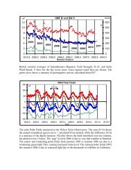
They showed that above a Hale portion of a SB, the green corona has a maximum inbrightness, while above a non-Hale boundary, the green corona has minimum brightness.Using synoptic maps of the magnitude of the photospheric field strength observed at Mt.Wilson Observatory during 1967 to 1973 it was also found that the unsigned magneticfield flux is at a maximum at the Hale boundary, in concert with the green coronabrightness.We have recently repeated the analysis using all available date from the Wilcox SolarObservatory (WSO). We superpose full-disk magnetograms from the times where a SBwas at [i.e. within a day] central meridian. We can take advantage of the polarity changesand treat (-,+) boundaries as (+,-) boundaries by reversing the sign of the magnetic field,and of the Hale magnetic cycle by reversing hemispheres between cycles to construct a‘nominal’ magnetogram for a (+,-) Hale boundary averaged over solar cycles 21-24,Figure 3.Figure 3. The average magnetograms for a nominal (+,-) Hale boundaryduring solar cycle 23. 910 magnetograms superposed on 765 SBs using theWSO observations 1976-2010. Some data has been mirrored and signreversedas described in the text to reduce all data to the situation for cycle23. The Hale portion of the sector boundary is marked by the semitransparentbar. Left Figure shows the average signed field, while the righthandFigure shows the average unsigned [total] field.It is now evident, that on average, what causes the ‘warps’ in the current sheet (anmdhence the SB at Earth) originates strongly from one hemisphere, namely that which hasthe Hale boundary (the Northern in Figure 3). Coronal holes are often found co-locatedwith the interiors of the sectors.One important (the only?) source of the open flux is dispersing flux from active regionswith strong magnetic fields so we expect the concentration of total flux at the Haleboundary as shown in the right-hand side of Figure 3. The closed field lines associated

with the active regions would trap coronal material, explaining the enhanced brightnessof the green corona at Hale boundaries.We would also expect flares and microflares to preferentially occur near the Haleboundary. Using the RHESSI flare list covering the interval March 2002 to March 2008(wholly within cycle 23) we find, indeed, that to be the case, Figure 4:Figure 4. Distribution of RHESSI flares on the day a SB was mapped back tocentral meridian for part of solar cycle 23, March 2002 to March 2008. Thered boxes show where flares are expected based on association with strongmagnetic fields: at the Hale boundary. The circles show that hardly any flaresoccur near a non-Hale boundary.GOES flares for May 1996 to January 2009 (cycle 23) show the same distribution, albeitwith much poorer statistics because of the smaller number of cases:Figure 5. As Figure 4, but for the GOES spacecraft, May 1996 to Jan. 2009.

We can quantify the asymmetry by integrating the count in longitude between 30 degreeson either side of Central Meridian, Figure 6:Figure 6. Number of flare events within ±30 degrees of Central Meridian as afunction of latitude.The correlation between the polarity of the solar Mean Field (over a smaller disk centeredon the sun-Earth point) and the polarity of the Heliospheric Magnetic Field maximizesfor a disk radius of 0.5 solar radius, justifying the choice of 30 degrees on either side ofCentral Meridian.In a sense, all this is trivial, i.e. just what we would expect, were it not for the fact that thesolar sector structure is very organized and long lived, indicating that solar activity is notrandom, but enjoys the same degree of spatial and temporal structure.