Session K.pdf - Clarkson University

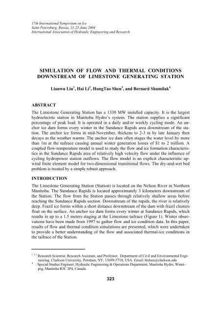
17th International Symposium on IceSaint Petersburg, Russia, 21-25 June 2004International Association of Hydraulic Engineering and ResearchSIMULATION OF FLOW AND THERMAL CONDITIONSDOWNSTREAM OF LIMESTONE GENERATING STATIONLianwu Liu 1 , Hai Li 2 , HungTao Shen 3 , and Bernard Shumilak 4ABSTRACTThe Limestone Generating Station has a 1330 MW installed capacity. It is the largesthydroelectric station in Manitoba Hydro’s system. The station supplies a significantpercentage of peak load. It is operated in a daily and/or weekly cycling mode. An anchorice dam forms every winter in the Sundance Rapids area downstream of the station.The anchor ice forms in mid-November, thickens to 2-3 m by late January thendecays as the weather warms. The anchor ice dam often stages the water level by morethan 1m at the tailrace causing annual winter generation losses of $1 to 2 million. Acoupled flow-temperature model is used to study the flow and ice formation characteristicsin the Sundance Rapids area of relatively high velocity flow under the influence ofcycling hydropower station outflows. The flow model is an explicit characteristic upwindfinite element model for two-dimensional transitional flows. The dry-and-wet bedproblem is treated by a simple robust approach.INTRODUCTIONThe Limestone Generating Station (Station) is located on the Nelson River in NorthernManitoba. The Sundance Rapids is located approximately 3 kilometers downstream ofthe Station. The flow from the Station passes through relatively shallow areas beforereaching the Sundance Rapids section. Downstream of the rapids, the river is relativelydeep. Frazil ice forms within a short distance downstream of the dam with frazil clustersfloat on the surface. An anchor ice dam forms every winter at Sundance Rapids, whichresults in up to a 1.5 meters staging at the Limestone tailrace (Figure 1). Winter observationshave been made from 1997 to gather flow and ice condition data. In this paper,results of flow and thermal condition simulations are presented, which were undertakento provide a better understanding of the flow and associated thermal-ice conditions inthe tailrace of the Station.1 2 3 Research Scientist, Research Assistant, and Professor, Department of Civil and Environmental Engineering,Clarkson University, Potsdam, NY, 13699-5710, USA. Email: htshen@clarkson.edu4Special Studies Engineer, Hydraulic Engineering & Operations Department, Manitoba Hydro, Winnipeg,Manitoba R3C 2P4, Canada.323

Fig. 1. Aerial view of the area from Limestone Generating Stationto Sundance Rapids and the anchor ice damWINTER OBSERVATIONS OF ANCHOR ICE FORMATIONField observations have been made by Manitoba Hydro since 1997. It has been observedthat the anchor ice dam staging effect generally starts in mid-November due to the suddenair temperature drop. The water discharge typically varies in daily cycles rangingfrom about 1,500 to 4,500 m 3 /s. Frazil ice attachment to the bed is usually the mainmechanism for anchor ice growth. Due to the daily cycling of the station outflow, theice dam is formed by a combination of anchor ice and aufeis growth. Anchor ice andborder ice upstream of the Rapids can release and contribute to the development of theice dam. The mechanisms that contributed to the ice dam formation in the SundanceRapids are considered to include: 1) anchor ice growth by frazil attachment and supercoolingeffect; 2) aufeis growth; and 3) anchor ice and border ice released from upstream.The resulting ice dam effectively closes off 80 to 90% of the channel width, restrictingflow except a few small opening slots and resulting in up to a 1.5 m increase intail water level at the station by the end of winter (Manitoba Hydro 2000).57.00056.000Elevation (m)55.00054.00053.000Observed Data onNovember 1999Open WaterRating Curve52.00051.0000.0 1000.0 2000.0 3000.0 4000.0 5000.0discharge (m 3 /s)Fig. 2. Limestone tailrace staging during November 1999324

57.00056.000Elevation (m)55.00054.00053.000Observed Dataon February 2000Open WaterRating Curve52.00051.0000.0 1000.0 2000.0 3000.0 4000.0 5000.0discharge (m 3 /s)Fig. 3. Limestone tailrace staging during February 2000Plots of tailrace elevation vs. water discharge, as show in Figures 2 and 3, are generatedfrom the recorded data for the months of 1999-2000 winter to show the anchor ice damstaging effect. It can be seen that the staging effect was less than 1 meter in November.It went up to more than 2 meters in February.THE NUMERICAL MODELA two-dimensional finite element numerical model with coupled hydrodynamic andthermal-ice components has been developed to simulate the flow as well as the watertemperature and frazil ice concentration of the river. The hydrodynamic sub-modelsolves the two-dimensional, depth-averaged, unsteady flow equations. The streamlineupwind Petrov Glerkin concept (Brooks and Hughes 1982, Hicks and Steffler 1992, andBerger and Stockstill 1995) is used in the finite element model with an explicit implementation.The model is capable of simulating transitional flows (Liu and Shen 2003).A simple technique is used to treat dry-and-wet bed conditions. A small flow depth andlarge bed resistance is automatically assigned to the dry area, so that the flow velocitiesat the ‘dry’ areas become negligibly small to approximate the dry bed condition. Themain component of the thermodynamic sub-model is to simulate the water temperature.A finite element model with optimum added viscosity is used for both water temperatureand frazil concentration.The model domain extends from the tailrace of the Limestone Generating Station todownstream of the Sundance Rapids. At the upstream boundary, i.e. the generating stationtailrace, the time-dependent water discharges are specified. At the downstreamboundary, water surface elevations are specified according to the rating curve developedin a previous study (Manitoba Hydro 2000). Several soundings were made in differentyears to provide data for channel bathymetry. Some discrepancies were found betweendifferent data sets (Manitoba Hydro 2000). Additional survey is being planned to resolvethese discrepancies before a detailed calibration can be made. The bathymetry andthe model domain used in the present simulation are presented in Figure 4. The blacklines indicate the sounding lines from field surveys.325

elevation_interp53.0052.5052.0051.5051.0050.5050.0049.5049.0048.5048.0047.5047.00Limestone G. S.Sundance RapidsFig. 4. Bathymetry used in the simulationThe first two days of November 1999 are simulated to demonstrate the capability of themodel in simulating cycling discharge with dry- and-wet bed conditions. Figure 5 showsthe comparison of simulated and observed water surface elevation at the tailrace alongwith the rating curve. Figure 6 shows the simulated water depth at a low flow (1000 m 3 /s)condition. Figure 7 shows the simulated water depth at high flow (3500 m 3 /s). It can beseen that during low flow, many parts of the river bed, especially at the Rapids, are exposed.The water discharge pattern at the tailrace, i.e. the upstream boundary condition isalso shown in Figures 6 and 7.Tailwater Rating Curve for no ice condition57.00056.000Elevation (m)55.00054.00053.000Observed Dataon Nov.1 toNov. 15, 1999Rating Curvesimulated52.00051.0000.0 1000.0 2000.0 3000.0 4000.0 5000.0discharge (m 3 /s)Fig. 5. Simulated water surface elevation at Tailrace326

(m 3 /s)50004000300020001000Hour 24:00:0000 12 24 36 48Time (hour)Water Depth (m)54.543.532.521.510.50.0100100020003000Limestone G.S.Sundance RapidsVelocity Vector1m/sZ(m)400045(m)0 500 1000 1500 2000 2500 3000605550Fig. 6. Simulated water depth and velocity at low flow (Q=1000 m 3 /s)(m 3 /s)50004000300020001000Hour 36:00:0000 12 24 36 48Time (hour)Water Depth (m)54.543.532.521.510.50.0100100020003000Limestone G.S.Sundance RapidsVelocity Vector1m/sZ(m)400045(m)0 500 1000 1500 2000 2500 3000605550Fig. 7. Simulated water depth and flow velocity at high flow (Q=3500 m 3 /s)327

It was observed that, from Nov. 16, 1999, the air temperature dropped suddenly (figure 8)and the staging effect developed. A 96-hour simulation was conducted, for the period ofNov. 16 to Nov. 19. A composite sine function is used to interpolate the daily maximumand minimum air temperature, as shown in Figure 8, to better reflect the diurnal air temperaturevariation. The staging and water discharge during this time period are shown inFigures 9 and 10. The water temperature and frazil concentration distributions are affectedby the air temperature variation and also by the water discharge cycling. The simulatedwater temperature and frazil concentration distributions, assuming that the water temperatureof the discharge from the station is 0.05 o C, are shown on Figures 11 and 12 at the endof the simulation (hour 96).50-5Generated CurveMaximumAverageMinimumTemperature ( o C)-10-15-20-25-300 24 48 72 96 120 144 168 192 216 240Time (Hours from Nov. 16, 1999)Fig. 8. Air temperature from Nov. 16, 1999CONCLUSIONSA coupled two-dimensional depth-averaged flow and thermal-ice model is developed.The flow model is capable of simulating mixed flow conditions with the capability oftreating dry-and-wet bed conditions with fluctuating discharges. The thermal-ice modelis capable of simulating water temperature and frazil concentration distributions. Themodel is applied to the tailwater of the Limestone Generating Station to simulate theflow and water temperature/frazil ice conditions. The model is to be extended to studythe formation of anchor ice dams in the Sundance Rapids area of the river reach.328

Tailwater Elevation vs. DischargeObserved Data on Nov.16-1957.00056.000Elevation (m)55.00054.00053.00052.000Nov.16Rating CurveNov. 17Nov.18Nov. 1951.0000.0 1000.0 2000.0 3000.0 4000.0 5000.0discharge (m 3 /s)Fig. 9. Staging effect of anchor ice development in Nov.16 to 19, 19996000.05000.0Water DischargeWater Discharge (m^3/s)4000.03000.02000.01000.00.011-15-99 11-16-99 11-17-99 11-18-99 11-19-99 11-20-99 11-21-99DateFig. 10. Water discharge variation from Nov. 16 to 19329

Hour 10:00:00 60:00:00 11:00:00 12:00:00 13:00:00 14:00:00 15:00:00 16:00:00 17:00:00 18:00:00 19:00:00 20:00:00 21:00:00 22:00:00 23:00:00 24:00:00 25:00:00 26:00:00 27:00:00 28:00:00 29:00:00 30:00:00 31:00:00 32:00:00 33:00:00 34:00:00 35:00:00 36:00:00 37:00:00 38:00:00 39:00:00 40:00:00 41:00:00 42:00:00 43:00:00 44:00:00 45:00:00 46:00:00 47:00:00 48:00:00 49:00:00 50:00:00 51:00:00 52:00:00 53:00:00 54:00:00 55:00:00 56:00:00 57:00:00 58:00:00 59:00:00 61:00:00 62:00:00 63:00:00 64:00:00 65:00:00 66:00:00 67:00:00 68:00:00 69:00:00 70:00:00 71:00:00 72:00:00 73:00:00 74:00:00 75:00:00 76:00:00 77:00:00 78:00:00 79:00:00 80:00:00 81:00:00 82:00:00 83:00:00 84:00:00 85:00:00 86:00:00 87:00:00 88:00:00 89:00:00 90:00:00 91:00:00 92:00:00 93:00:00 94:00:00 95:00:00 96:00:00Velocity Vector1m/sWater Temperature0.050.040.030.020.010-0.01-0.02-0.03-0.04-0.05Sundance RapidsAir Temperature ( o C)0-10Limestone G.S.-20-300 12 24 36 48 60 72 84 96Time (hour)Fig. 11. Simulated water temperature distributionHour 96:00:00 10:00:00 60:00:00 11:00:00 12:00:00 13:00:00 14:00:00 15:00:00 16:00:00 17:00:00 18:00:00 19:00:00 20:00:00 21:00:00 22:00:00 23:00:00 24:00:00 25:00:00 26:00:00 27:00:00 28:00:00 29:00:00 30:00:00 31:00:00 32:00:00 33:00:00 34:00:00 35:00:00 36:00:00 37:00:00 38:00:00 39:00:00 40:00:00 41:00:00 42:00:00 43:00:00 44:00:00 45:00:00 46:00:00 47:00:00 48:00:00 49:00:00 50:00:00 51:00:00 52:00:00 53:00:00 54:00:00 55:00:00 56:00:00 57:00:00 58:00:00 59:00:00 61:00:00 62:00:00 63:00:00 64:00:00 65:00:00 66:00:00 67:00:00 68:00:00 69:00:00 70:00:00 71:00:00 72:00:00 73:00:00 74:00:00 75:00:00 76:00:00 77:00:00 78:00:00 79:00:00 80:00:00 81:00:00 82:00:00 83:00:00 84:00:00 85:00:00 86:00:00 87:00:00 88:00:00 89:00:00 90:00:00 91:00:00 92:00:00 93:00:00 94:00:00 95:00:00Velocity Vector1m/sFrazil Concentration (%)0.50.450.40.350.30.250.20.150.10.050.010Sundance RapidsAir Temperature ( o C)0-10Limestone G.S.-20-300 12 24 36 48 60 72 84 96Time (hour)Fig. 12. Simulated frazil ice concentration330

REFERENCESBerger, R.C. and Stockstill, R.L. Finite-element model for high-velocity channels. Journal of HydraulicEngineering, 121(10), ASCE, 710-716 (1995).Brooks, A.N. and Hughes, T.J.R. Streamline upwind Petrov Galerkin Formulations for Convection DominatedFlows with Particular Emphasis on the Incompressible Navier-Stokes Equations. Computer Methodsin Applied Mechanics and Engineering, 32, 199-259 (1982).Hicks, F.E. and Steffler, P.M. Characteristic dissipative Galerkin scheme for open channel flow, Journalof Hydraulic Engrg, ASCE, 118(2), 337-352 (1992).Liu, L. and Shen, H.T. A Two-dimensional Characteristic Upwind Finite Element Method for TransitionalOpen Channel Flow. Report 03-04, Department of Civil and Environmental Engineering, ClarksonUniversity, Potsdam, NY (2003).Acres Manitoba Limited. Limestone Ice Mitigation Study. Report submitted to Manitoba Hydro. Winnipeg,Manitoba, May (2000).331

17th International Symposium on IceSaint Petersburg, Russia, 21-25 June 2004International Association of Hydraulic Engineering and ResearchEXPLOITING SPECIFICS OF THE HYDRAULIC ENGINEERINGSTRUCTURES OF THE WATER POWER PLANTS IN WINTERPERIODA.G.Vasilevsky 1The experience which was received for many years of the hydraulic engineeringstructures exploiting let to provide of their safety exploitation and to create the safetycomplete sets and constructions as the system of the normative base standards.80-years period of the mass building of the water power plants which is beginning fromthe GOELRO-plan we can divide in two steps.On the first step usually were constructed a not high power water power plants withderivative tape of construction which let to use the low height dams for this purpose. Someof them like Kondopojskaya water power plant in Karelia, Niva-2 water power plant on theKola peninsula and the most water power plants which are located in Caucasus region andin Central Asia. The exploitation specifics of the derivative water power plants in winterperiod connected with problems of the struggle with an ice forming inside of water and iceand shuga influence on waterways of the water power plants like: channels, water intakestructures of the water power plants, ice outlets and shuga outlets. In this time worked upthe ways of the struggle with ice and shuga for providing of capacity for work of equipmentof the water power plants which are usually were not unified into power engineeringsystems. This water power plants were enough autonomous units of the electric powersupply for their regions which made them too responsible for this purpose.The struggle with ice and shuga we can divide on active and passive ways. The activeway of the struggle was directed on preventing of the negative influence of ice andshuga on the water power plants like creation of the special complete sets ofconstructions, the heating systems and the passing regimes.The passive way including the struggle with consequences of the anchor ice damforming, the blocking up of the water conduits and the ice covering of the mechanicalequipment.On the first step (from 1920-s to 1940-s) usually was used the passive way likemodernization of the mechanical equipment which was used for liquidation of1 The B.E. Vedeneev All-Russian Research Institute of Hydraulic Engineering (VNIIG), Gzhatskaya str., 21,St.Petersburg, Russia.332

consequences of the blocked up turbine gratings, organization of the heating supply (hotwater, steam and others).Organization of ice-protected walls (like on the Volkhov and Nizhne-Svirskaya waterpower plants) played their own role in protection from the ice but did not give the realresults in the struggle with the ice inside of water and with shuga. The pump settlingbasins which were widely used on mountain rivers (The Chiriksky cascade of the waterpower plants in Central Asia) also did not give the real results in settling and passing ofshuga.Worked up the system for the heating of turbine gratings (direct electric power throughthe pivots, inductive method for the heating of pivots and others ). Was shown thelimited possibility of this systems but anyway they were projecting and installing evenduring the second constructing period of water power plants. So, for example, on theKuibyshevskaya water power plant (as on the V.I.Lenin Volzskaya water power plant)which was opened for exploitation in 1960-s the originally designed system for theheating of gratings later was removed out of the structure.The rich experience was received on power engineering systems located in the North-West part of Russia during all this time (on the Leningrad, Karelia and the Colapeninsula power engineering systems). The Volkhov water power plant several timeswas stopped from the blocking up of turbine gratings with the shuga .After that theupper sections of construction were removed out of the structure for the heating process.Today this problem completely solved by using of the intensive complete freezingwhich was realized by removal of water power plant out of the daily head regulationwith deducing of discharges (speeds of the stream).After that the ice inside of water cancome to the surface and organize the complete freezing forming process. All thisinformation was shown in instructions for exploitation of the hydraulic engineeringstructures. Establishment of the ice cover in reservoirs and waterways as one of themost effective (active) action was used in the first winter period of the water powerplant exploitation. Later this method was widely used in all exploiting system of thewater power plants. But some mistakes of the operating personnel in using of this actionreduced to the hard accidents. As a good example of that was a situation on the Niva-2water power plant which belongs to the Kolenergo power engineering system. Forinstallation of the complete freezing was used the wooden pivots in the waterway. Laterthe wooden pivots under loading oscillations was moved with an ice to the water intakestructure and completely blocked up the waterway. The solving of this problem on theNiva-2 water power plant was founded in 1960-s when the large enough Kolenergopower engineering system was formed.Was determinated that absolutely possible to avoid of the ice forming inside of water inwaterway by the growing of speed of the stream and by cutting off the time of coolingprocess of enough “hot” water which was taken by the Niva-1 water power plant fromreservoir of the lake of Imandra. This method also was used on the Sevano-Rozdanskycascade of water power plants in Armenia.On the second step of construction of water power plants in the Soviet Union (postWorld War II period in 1960-s and 1970-s) usually were constructed the middle sizeand the large size water power plants on the Volga and Dniper rivers as in Kazhakhstanand in Siberia with large reservoirs and high enough dams (more than 20 meters high).The problems which was connected with the ice forming inside of water and with333

influence of the shuga on waterways is almost gone now (become with a not high ofprobability).But the problems which is connected with the ice influence on the damgates were retained. If construction of water power plants is calculated with an iceloadings, so in this case the gates must be protected from the ice pressure. During thistime were elaborated and installed the methods for the holding of polynya infront of thegates. The basic methods now which are using for the holding of polynya by thebarbotage structures infront of the gates with using of air which is going from the sill ofthe gate along the pressure face, or holding of polynya by the stream-forming structureswhich give the jet of water along the pressure frontage. Determined all conditions forusing of this methods. Also was determined that this methods are effective with thepresence of the temperature stratification infront of the gates.Another very seriously problem of exploitation of the hydraulic engineering structuresand their equipment during winter period was the serving of possibility of the waterdropping in winter period. Usually it connected with regulation possibilities ofreservoirs with providing of work of the water power plant cascade in case if on one ofthe water power plants the working equipment was out of work , as in case of repairwork of the broken equipment or if equipment was stopped with necessity for thepassing of water according to sanitary or other reasons. In the most cases the passing ofthe flood realize with the high enough temperature of air outside of winter period.For providing of winter exploitation of water power plants we need the heating of theslot constructions and protection of pressure face of the gates from underwater icecovering. For the solving of this problems we have enough of home and foreignexperience in this field. Methodic for the heating of the slot constructions just the samelike for the gratings: direct electric power, inductive electric heating, oil heating orother. Now we have the problem with reconstruction of the heating systems which wereout of work. In this field we have brand new elaborates which were created in theB.E.Vedeneev All-Russia Research Institute of Hydraulic Engineering. This newelaborates were created on the base of using the silicon organic elements. Their usingfor reconstruction of the heating systems which was out of work made this problemmuch easy because now we do not need the expensive repair works which in the mostcases connected with replacement of the different parts of construction. This newelaborates made the completely new situation for using of the modern methods inoptimization of electricity discharges for the heating process by installation automaticcontrol systems with a program supply which is operate depends from our decision.Today we can say that exploitation of the hydraulic engineering structures in winterperiod connected with technical solutions which we can choice depends from conditionsand different tasks of exploitation. Very important to develop methods for prognosis ofexploitation conditions: hydrometeorological and technological.Prognosis of hydrometeorological factors is a very difficult problem. For the solving ifthis problem not enough to have a list of the statistic observations. Manifestation of thehydrometeorological factors depends not just from the complete set of construction andtechnical solutions but from the exploitation regimes in the most cases.During winter exploitation of the hydraulic engineering structures we must to use theactive ways in struggle with different negative influences. Very important to usedifferent ways in control of the negative influences on the first step of projecting of thehydraulic engineering structures with using of all exploitation experience in this fieldand most which was used in winter period.334

17th International Symposium on IceSaint Petersburg, Russia, 21-25 June 2004International Association of Hydraulic Engineering and ResearchENSURING OF OPERATION OF WITHDRAWALSIN FRAZIL-ICE CONDITIONSI.N.Shatalina, 1 G.A.Tregub 1 , N.S.Bakanovichus 1ABSTRACTOn the rivers with a long period of ice flow, difficulties in water collecting can occur.The purpose of this paper is working out hydraulic ways of withdrawal strainer protectionagainst frazil and avoiding supercooling effect inside the system. This paper concernsdifficulties arising in the operation of river withdrawals situated in the frazil producingriver stretches. Methods of calculations of frazil flow parameters are given. Theconstruction of water strainers of umbrella-like type and system of collector well heatingon the basis of compositional resistive materials (CRM) ensuring safe operation ofwithdrawals in frazil-ice conditions are proposed. The results of experimental analysisof the new strainer construction and the parameters of the new heating system of thewater collector well are represented.METHOD OF ESTIMATION OF WATER SUPERCOOLING AND FRAZILDISCHARGE COMING INTO WITHDRAWALSOn the large rivers like the Neva and the Amur the period of autumn frazil flow cancontinue rather long, sometimes up to more than a month. In the period of frazil flowand the beginning of freezing-up there are plenty of polynyas – ‘factories of frazil’. Atthis time withdrawals can have ice difficulties connected with blocking of the strainerwindows with passing frazil and their freezing in supercooled water. The method of estimationof water supercooling and frazil discharge coming into water collectors isbased on the Pekhovich model (Pekhovich, 1983). According to this model a fewstretches along the river can be described, every of which has a definite number of icethermal parameters: 1) the stretch of water supercooling to the section of inside waterice formation; 2) the stretch going from this section to the section of frazil flowing up;3) the stretch of growing supercooling to the section of maximum supercooling ; 4) thestretch of supercooling decrease to the section of maximum intensification of inside waterice formation; 5) the stretch to the ice edge. The mentioned stretches are separatedfrom each other with distinct sections and have the definite water temperature t , its gra-1The B.E. Vedeneev All-Russian Institute of Hydraulic Engineering (VNIIG), Gzhatskaya str., 21,St.Petersburg, Russia.335

dtdient along the flow , the concentration of surface frazildx, intensity of frazil formationS , frazil discharge Q and its gradient along the flowffβ fdQ fdx(table 1) (Pekhovich,Tregub, 1980; Tregub, 1997). The detailed method of estimation of the mentionedsection positions was given in (Tregub, 1977).Table 1. Ice Thermal Conditions for Typical Sections along River Flow№ Sectiont,oCdtdxoC,mParameters of ice thermal stateβ fWtS f ,s3mQ f ,sdQ 2 f m,dx s1 Zero isotherm 0 03 Beginning of frazilflowing up 04 Maximum of watersupercooling 0 >00< β f 0 >0 >06 Ice edge ∼ 0 ≥0 ∼ 1 ≥0 ≥0 ∼ 0The position of the maximum supercooling section is calculated with the formulawhereP x.maxxmax2 h=bLv.fα1⋅V⋅ P( − ϑ )ex.max, (1)dimensionless parameter taken from the following relations:Px.maxβ f .maxP−β f .max − ln( − β )= 1 , (2)f max( P +1) 2 −1= −P max + max , (3)maxα1b=2 Lv.f( − ϑ )⋅Vehb, (4)α1,ϑ e– heat transfer coefficient and equivalent air temperature (Recommendations,1986); b – width of the flow: V – flow speed; – initial ice thickness (Recommendations,1986);L v. fh b– volumetric latent frazil formation heat.336

The position of the section of maximum intensity of frazil formationanalogously withxmaxx m. f, but using β m. f instead of β f . max in formula (2)is calculated23β m.f = Y − Px.max, (5)Y = U 1 + U 2 , (6)3 2 21 2 w1± w1w 2U , = + , (7)2⎛⎞⎜cvQw 1 = P⎟x . max0,296 Px.max − 0,67 −2, (8)⎝α1b⎠2( 3 )w = + , (9)2 −0,22 P x .max 2 Px.maxc v – volumetric thermal capacity; Q – river water discharge.The water temperature in the stretch between the section of maximum supercooling andmaximum frazil formation intensity can be found with help of the relation (Tregub, 1997):( 1− β )⎛xx⎞max⎜ α b1 f ⎟⎧1t = exp −∫ dx ⎨ ∫ [ α b ( 1−β) ϑ +1⎜ ⋅ ⎟f ec⎝ 0v Q⎠⎩cvQ0( 1−β)⎛xmax⎞ ⎫2⎪]⎜ α1b f+ L ⋅ β⎟v.f v hbf exp⎜ ∫dx⎟dx⎬. (10)cvQ⎝ 0⎠ ⎪⎭The frazil discharge which can get into the withdrawal Q f.w is calculated on the basis ofthe assumption that after getting into the strainer the water supercooling disappearscompletely:cvQw⋅ ∆ tQ f .w = − . (11)LWhere Q w – water discharge coming into the strainer; ∆t – water supercooling comparedwith 0 C. The given formulas were used for calculation of water supercooling andºfrazil discharge on the section of the strainers.There have been tried a lot of ways to prevent frazil getting into withdrawals (e.g. withusing compressed air, electrical heating of the strainer windows). But as a rule thoseways are too expensive and consume great quantity of energy for heating. Even in caseof avoiding ice formation on the strainer windows, supercooled water gets inside andafter crystallizing into frazil it blocks the water-supply system. As a result of a scientificanalysis of different protections a hydraulic way of preventing frazil and other impuritiesgetting into withdrawals was chosen, which allowed creating an umbrella-like typeof strainers with a hydraulic vortex motion under the withdrawal cap.Using hydraulic vortex motion for controlling oil impuraties and frazil. Using hydraulicway of controlling impurities and frazil at the strainers is based on the creation avortex motion at the withdrawal entry. This motion keeps different type of floating im-337v. f

purities from getting into the withdrawal with help of umbrella-like strainers and a ‘hydraulicround-about’, which spins water by pumping it through tangential-oriented pipes(Shatalina, etc., 1994). The impurities getting into the flow are carried out from underthe withdrawal cap. The proposed version of a ‘hydraulic round-about’ can protect oilimpurities, frazil, whitebaits, water plants, etc from getting into withdrawals. The constructionof the ‘hydraulic round-about’ under the cap of the umbrella-like strainer isshown in fig.1.Fig.1 The construction of the ’hydraulic round-about’ under the cap of the umbrella-like:1 – the cylindrical part of the withdrawal cap; 2 – the strainer;3 – the pipe, delivering water to the ‘hydraulic round-about’; 4 – L-shaped nozzlesExperimental investigations of the ‘hydraulic round-about’. Investigations of the‘hydraulic round-about’ was performed on the withdrawal model scaled downas 1 to 23. With the diameter of the ‘umbrella’ 0,280 m and its height 0,191 m.Underthe ‘umbrella’ there were two tangential-oriented nozzles with diameters 0,012 m. Thewater discharge of the withdrawal was 0,2 – 0,5 l/sec, the discharge of the ‘hydraulicround-about’ changed from 0,1 to 0,5 l/sec. The equipment was built in the availablehydraulic test bench, which had a delivery tank (with the fall of 2 m), a supply and aworking part of 2,0 x 0,58 1,26 m in size, two centrifugal pumps with discharges 10l/sec and 3 l/sec. Water delivered both to the working part of the bench imitating a riverflow and to the ‘hydraulic round-about’. The pump with the larger discharge kept thetank water level constant and the second pump imitated the pump collecting water fromthe river. The water discharges were adjusted with help of measure diaphragms accordingto the difference of the piezometer levels. The accuracy of the discharge measurementwas 0,5 – 1,5 %.338

The purpose of the tests was to define the range of the operation parameters of the‘round-about’ with different concentration of impurities coming under the withdrawalcap. These are the parameters which were varied during the tests: the discharge of the‘hydraulic round-about’; the initial concentration of the impurities withdrawal discharge; the vertical position of the tangential nozzles. In the result of the tests the quantityof the impurities both driven away from under the cap and accumulated under thewithdrawal cap were found. For three different positions of the nozzles 3 series of testswere performed. Except this the tests were carried out for both the active and inactivewithdrawal. Polyethylene of low pressure with density 970 kg/m 3 and particle diameters3–5 mm was used to model impurities and frazil. The masses of the particles bothdriven away from the withdrawal and accumulated under the cap were weighed on ascale with 0.01 g accuracy. The effect of the operation of the ‘hydraulic round-about’was estimated according to the mass of the impurities driven away from under the withdrawalcap. The impurities amounted 2–10% of the water mass coming into the withdrawal.The greater amount of impurities came under the withdrawal cap the greaterpercent of the initial mass was driven away from under the cap as a result of operatingthe ‘hydraulic round-about’. The direction of the ‘hydraulic round-about’ jets (clockwiseor anticlockwise) and its position comparatively with the ceiling of the ‘umbrella’as well as with the end of the collector pipe under the ‘umbrella’ and the lower edge ofthe ‘umbrella’ proved to be very important parameters. Using the data in fig.2, the influenceof the parameters can be estimated.7060The impuritiesdriven awayfrom underwithdrawal cap, %504030201000 0,02 0,04 0,06 0,08 0,1 0,12T he c onc e ntra tion of the im puritie sAnticlockwise with the inactive withdrawal;Anticlockwise with the active withdrawal;Clockwise with inactive withdrawal;Clockwise with active withdrawalFig.2. The dependence of the emission of impurities from underthe withdrawal cap in percent from the concentration of impuritiesin the flow and direction of the ‘hydraulic round-about’ jets(the cap is located 0,0515 m above the withdrawal;water discharge of the ‘hydraulic round-about’ is 0,24 l/sec)Among other factors, the greater quantity of impurities come with water the greater percentof them is driven away from under the withdrawal cap and the water coming intothe system is freed of them better. With any quantity of impurities coming under thewithdrawal cap, the effect of ‘round-about’ operation is 12 - 20 % higher if the tangential-orientednozzles are directed anticlockwise. The further tests were performed withthe anticlockwise nozzles and the fact will not be mentioned any more. With the inac-339

tive withdrawal the efficiency of the impurities removal is about 10 % higher than withthe active one. If there are a few withdrawals, this fact allows cleaning the area underthe withdrawal cap when one of the withdrawals is inactive. Using this model and thegiven size of the strainer more than 60 % of the impurities can be removed from underthe withdrawal cap in this way.The influence of the umbrella ceiling position in reference to the collector position isseen well in fig.3. The analysis of the given curves shows that the removal of the ‘umbrella’ceiling 0,08 m from the strainer level leads to the extremely low efficiency of the‘round-about’ (the emission of the particles is about 30 %). The reduction of the distanceto 0,05 m increases the efficiency almost twice. The further reduction of this distanceto 0,03 m does not practically influence the efficiency. Three different verticalpositions of the tangential-oriented nozzles of the ‘hydraulic round-about’ were tested,which showed the lower position was impractical, since the jets went from under the‘umbrella’ without creating the effect of water acceleration under the withdrawal cap.As to the upper position, in this case the nozzles were situated too close to the strainerswindows that made extra impurities get inside the system. After that all the further testswere performed with the middle position of the nozzles. In addition two positions of thenozzles along the ‘umbrella’ diameter were tested: in 5cm from the ’umbrella’ edge andclose to the collector pipe. The latter position proved to be ineffective. In the test theparticles moved actively vertically, but the absence of the horizontal movement did notdrive the particles from the strainer. That is why the main and recommended position ofthe nozzles close to the ‘umbrella’ edge was chosen.The impurities fromunder withdrawal cap, %7060504030201000 0,05 0,1 0,15The concentration of the impuritiesdistance 5,15 sm;distance 3,16 sm;distance 8,00 smFig.3. The dependence of emission of impurities from under the withdrawal cap in percentfrom their concentration in the flow with different positions of the cap over the activewithdrawal and the water discharge of the ’hydraulic round-about’ 0,24 l/secThe developed type of the strainer does not allow suspended impurities and frazil to getinside the system. Supercooled water, however, can get there freely. For controlling thefrazil formation inside the water supply system, collector well heating is proposed touse to avoid supercooling. Different kind of wells can be used for this purpose, where ablock of heaters can be installed. Crystallization starts when supercooled water gets intothe pipe leading from the strainer to the collector well. As frazil particles grow they beginto flow up. The size of ice particles, when the process of their flowing up starts isdefined by the expressions given in (Zakharov, Beilison, Shatalina, 1972) at the flowspeed 1,23 m/sec and Shezy coefficients 40,9 m 0,5 /sec. According to those relations the340

size of the flowing up particle is d f =7,5 mm. The time needed for the particle to reach thesize d f =7,5 mm can be found by the empiric formula of D.N.Bibikov (Tregub, 1997)τf=0,345( 0,5 d )1,5f0,47( 0,96⋅V+ 0,32 ( − t )At the maximum possible supercooling t w = –0.04 °C,) w. (12)τ f = 381 sec. For example, if thelength of the pipe is 120 m water passes it in τ t = 100 sec. In this time the particles offrazil formed in the supercooled water according to formula (12) grow to diameterd t = 3 mm. In the delivering pipe as frazil forms supercooling reduces. As a result thewater temperature coming into the collector well can be estimated by the followingformula:⎛ d ⎞3t t 1t⎛ ⎞= в ⋅ ⎜ − ⎟ = ( − 0,04) ⋅ ⎜1− ⎟ = −0,024 °С.d⎝ f ⎠ ⎝ 7,5 ⎠When water gets into the collector well the flow widens, supercooling disappears andintensive inside water ice formation starts. To prevent blocking of the collector wellsMO-2 with frazil it is necessary to give the water as much heat as needed to get rid ofthe supercooling. For carrying out of the listed tasks both the power and the type of theheater for operation of the collector well is necessary to determine. The necessary powerof the heater is found on the basis of the thermal balance equation, according to whichthe heating power is used for both increasing the water temperature up to t 0 = 0 °C andthe thermal output into the air:c Wτ( t − t ) + α F ( t − ϑ)( t − t )v s0 w=0e01 0+ λe⋅ F Nδ, (13)Wwhere W – the water collector well volume; τ 0= – the time of water exchange in theQ2πd well; t w – water temperature at the well exit (t w ~0,5° C); F = w– the area of the well4water-air contact; ϑ – air temperature; concrete thermal conductivity; λ e – heat concluctivityof concrete; ts – average long term soil temperature of the river floor; δ e –concrete well wall thickness. For the collector well with the diameter 4 m , the height9 m, the wall thickness 0,5 m and the temperatures ts = 4 o C, ϑ = –26 o C the necessarypower of the well heating is N = 127 kWt. The heating zone is to be located on the wellfloor close to both water delivering and withdrawing holes. Free convection developedin the water because of the heat coming up from the heater situated in the lower part ofthe well is favourable to the water temperature increase and the frazil melting. Forsteady-state heating of the collector wells the system consisted of flat heaters with activeelements made of compositional resistive materials (CRM) is worthwhile using.With the power of the well heating equal 127 kWt, 64 kWt are necessary for the heatingof the side well walls in the zone of water delivering and withdrawing and 63 kWt areneeded for the floor heating. Active heating elements developed by the authors andmade up of different CRM are proposed to be used. As one of the possible solution aspecial material with positive coefficient of resistance-temperature dependence is sug-341

gested. The material is composed on the basis of astringent bitumen with electrical conductiveand inert additions (electrical conductive bitumen – ECB) (license application№ 2002118348, priority of 08.07.2002, the positive resolution for license presentationof 08.01.2004). The principle of the material action is as follows: the resistance is retainedquite small till the temperature reaches the value, above which the resistancegrows quickly with the temperature growth. As this takes place, the resistance growth ismuch quicker than the growth of the temperature and the reduction of the current intensityassists it. It leads to the reduction of the heater consumed power. By contrast in caseof the system cooling the resistance lowers and the heating grows.Fig. 4. The dependence of ECB resistivity from the heating temperatureSo more intensive heating takes place in the more cooled areas, which leads to the constanttemperature of the whole system. Owing to such a self-regulation of the electricalcharacteristics of the material no special electrical systems of regulation are needed toheat the well. Furthermore in this case the overheating of neither the most active elementin the heater or the well itself is impossible. The recommended maximum temperatureof the active heating ECB element is +90 °C. One more advantage of the proposedmaterial is the fact that the latter can be used in the wide range of moisture contentup to the using it in water without changing its electrical parameters. One of thepossible heaters with ECB consists of six active heating elements of 100x200x40 mm insize and with nominal power 0,25 kWt, connected in series and placed in the metal box.Such a heater is of 650x270x50 mm in size and has a power 1,5 kWt and operates at thevoltage 220 V. Except ECB active heating CRM elements made of astringent phosphatecan be used in the heaters. Such a heater consists of 10 active elements connected in seriesof 650x270x50 mm in size, has the power 1,0 kWt and the operating voltage 220 V.The recommended maximum temperature of the active heating element of this type is100 °C. The It is worth noting that using CRM allows creating the heaters operating inthe wide voltage range. The arrangement of the heating elements in the heater can bedifferent. For ensuring both electrical and hydro isolation special mastic is poured intothe heater box. The exterior heater surface is covered with anticorrosive coating. It isrecommended to connect the heaters across since in this case even if one or more heatersfail the whole system continues operating. The warming up system of the collectorwell is to be automatically switched on as the water temperature at the end of the deliveringpipe is –0,01 °С and switched off as it is +5 °С.342

The combined usage of the umbrella-like strainers with the ‘hydraulic round-about’ andthe heating system of the collector wells will allow avoiding frazil-ice difficulties at thewithdrawals.REFERENCESPekhovich, A.I., (1983) The Foundations of Hydraulic Ice Thermal Engineering. Leningrad, Energoatomizdat,1983.Pekhovich, A.I., Tregub ,G.A., (1980) The Calculation of Frazil Formation and Ice Edge Movement inthe Downstream of Hydro Power Stations, Isvestia VNIIG, vol.143, 1980.Tregub, G.A., (1997) The Calculation of Thermal and Ice Operating Conditions as a Basis of ThermalConjunction of the Pools, Isvestia VNIIG, vol.230, part 2, 1997.P-28-86, VNIIG, (1986) Recommendations on the Calculation of the Downstream Polynia Length forHydro Power Stations, Leningrad, VNIIG, 1986.Shatalina, I.N., Tregub, G.A., Krasntskiy, A.R., Yakovlev, V.V., (1994) Hydraulic Way of Protection Withdrawalswith Umbrella-Like Collectors from Blocking with Frazil, Publications of Conferences and Sessionson Hydraulic Engineering “Thermal and Ice Environmental Aspects in Hydro Energetics”, (Ice-93),VNIIG, St.Petersburg, 1994.Zakharov, V.P., Beilinson, M.M., Shatalina, I.N.,(1972) The Nature of Ice Formation on the Rivers andReservoirs of Central Asia, Publications of the Second International Symposium on Ice by IAHR, Leningrad,1972, pp.246 – 250.343

17th International Symposium on IceSaint Petersburg, Russia, 21-25 June 2004International Association of Hydraulic Engineering and ResearchTHE NUMERICAL MODELING OF HYDRO-ICE-THERMALPROCESSES IN RESERVOIRSV.I. Klimovich 1 , V.A. Prokofiev 1 , I.N. Shatalina 1 , G.A. Tregub 1ABSTRACTMathematical modeling of hydro-ice-thermal processes has been considered in a numberof papers (e.g. Wake and Rumer, 1979; Alexandrov et al, 1992). In this paper atime-dependent 2D (plan) model of ice-thermal processes is viewed, in which for theprocess of ice cover formation the first approximation of uneven temperature profile (indepth) is taken into account. The algorithm of numerical solution of hydro-ice-thermalproblem was worked out and its verification was carried out. The numerical results ofthe hydro-ice-thermal regime and their comparison with the in-situ data of the Volga-Don NPP reservoir-cooler are given.MATHEMATICAL MODELThe conservative form of the shallow water equations with due regard for the friction onthe bottom, the wind influence and Coriolis’ forces looks like∂ h∂ t+∂ Q∂ x+∂ Qx y=∂ yq; (1)⎛2∂Q ⎞x ∂⎛ ⎞⎜Q ∂ QxQxy⎟∂Hτ∂h+ ⎜ ⎟bx τ wx 1 τ xx 1+= -gh + Ω + + +∂ ∂cQy-t x ⎝ h ⎠ ∂y⎝ h ⎠ ∂xρwρwρw∂xρw⎛2∂Q ⎞y ∂ ⎛ QxQy⎞ ∂ ⎜Qy⎟ ∂Hτ by τ wy 1 ∂hτyx 1+ ⎜ ⎟+ = -gh − ΩcQx-+ + +∂t∂x⎝ h ⎠ ∂y⎜ h ⎟ ∂yρ ρ ρ ∂xρ⎝ ⎠w w wwQx+ Qy1 1Qx = hux, Qy= hu y , τ bx = ρwC Qx, τ by = ρwC Qy, Ccur= g, C = h6,2 2C h n2 −2⎛z ⎞ 2τ wτ wx = τ w cos θw,τ wy = τ w sin θw,τ w = ρaκ ln ⎜ ⎟, z0= 0, 0144zW⎝ 0 ⎠ρagThe averaged in depth shear stresses τ xx , τ xy , τ yx , τ yy can be represented in the form (theindexes i, j correspond here to x, y)22∂hτ∂y∂hτxy∂yyy(2)(3)1 All-Russian Research Institute of Hydraulic Engineering (VNIIG), Gzhatskaya str., 21, St. Petersburg,195220, Russia344

hτιj⎡∂(hu∂ ⎤i ) (hu j )= ν t ⎢ + ⎥ .ρw⎢⎣∂ x j ∂ xi⎥⎦Here h – water depth; H=h+z B – the level of the free water surface; z B – the bottomlevel; u x , u y – the projections of the averaged (in depth) velocities on the axes x, y;Ω c = 2ω sinϕ – Coriolis’ parameter; ω – angular velocity of the Earth rotation; ϕ – thearea latitude; g = 9.81 m/s 2 – the acceleration of gravity; ρ w – the water density; ρ a – theair density; τ bx ,τ by – the projections of the friction forces on the axes x, y; ν t – turbulentviscosity coefficient; C – Chezy coefficient; n – roughness coefficient; С cur – thecoefficient of the bottom friction owing to the flow; τ wx , τ wy – the projections of thewind shear stress on the axes x, y; θ w – the angle between the wind direction and theaxis x; κ = 0,4 – Karman’s constant; W – the wind speed on the height z (compared withthe surface level); z 0 – the roughness coefficient of water surface; q(x, y) – the intensityof the mass source in the point with the coordinates (x, y). The viscosity coefficient ν tcan be determined on the basis of the Prandtle’s model−12 2ν = κ h , u = ρ ( τ + τtu* *The heat transfer equation in the context of the 2D (plan) model is derived on the basisof the averaging in depth 3D equation of transferring and has a formwbxby) .∂Th∂Thu+∂t∂xx∂Thu+∂yy=∂ ⎛ ∂T⎜ µTh∂x⎝ ∂x⎞⎟⎠∂ ⎛ ∂T+ ⎜ µTh∂y⎝ ∂y⎞⎟⎠1+ (ΦSρ wc w+ ΦB+ q ) . (4)THere T – averaged (in depth) water temperature; µ T , µ T – the total thermal diffusivitycoefficient with regard to dispersion; c w – specific heat of water; Φ S – the heat-fluxdensity on the water surface; Φ B – the heat-flux density on the bottom; q T – the intensityof the internal heat sources. The calculation of the heat-flux density Φ S is performed onthe basis of (Methodic Recommendation, 1976; Recommendation, 1979;Recommendation, 1986).The changing of the ice thickness on the water surface is determined according to therelationd hIρ I L = Φ SI – Φ IW . (5)d tHere ρ I – the ice density; L – the latent melting heat; h I – the ice thickness; Φ SI – theheat-flux density on the boundary of ice-air (from ice to air); Φ IW – the heat-flux densityon the boundary of ice-water. The relation (5) is used in two cases – when there is alreadyice cover (h I > 0) or when the calculated surface water temperature T SW gets lowerthan the temperature of water freezing (T SW

It is significant that the radiation thermal transferring, the evaporation transferring andconventional transferring are all taken into account when Φ SS (Φ SI ) is calculated accordingto (Recommendation, 1986).The surface water temperature T SW (without ice cover) as a first approximation is determinedin the assumption of the linear character of the heat flux changing along thedepthh hTSW= T + ΦSW−ΦBW. (6)3λWZ6λWZHere λ WZ – the thermal diffusivity coefficient in the vertical direction; Φ SW – the heatfluxdensity on the boundary of air-water; Φ BW – the heat-flux density on the bottom ofthe reservoir. Since the relation (6) is only used with the proviso that ice formationstarts on the water surface (T SW

length was ≈800 m, its average width – ≈80 m, its average section area – ≈300 m 2 . Thetotal thermal diffusivity coefficient with regard to dispersion was supposed to be proportionalto the unit discharge µ = α(Q+ Q + 0.14 ⋅10m /s and was determined on2 2 1/2−6 2theTx y )basis of the in-situ data for the period from October 16, 2002 to December 8, 2002 (whenthere was no ice cover on the reservoir). In Fig.1 the comparison of the calculated andthe in-situ data of the water temperature on the entrance of the NPP is shown.The presented data on modeling of the hydro-ice-thermal situation in the Volga-DonNPP cooler reservoir for the period from October 16, 2002 to January 12, 2003 (whenthere was full average day meteorology data) showed that the beginning of ice formationin the reservoir was on December 1. According to the in-situ data the first shore icein the area of the additional water pump station (AWPS) was observed on December 1and the ice cover formation in the area of AWPS started on December 5. According tothe calculations an ice formation in the intake channel began on December 10. As forthe in-situ data the first shore ice formation in the intake channel took place on December9. The maximum ice thickness in the period was observed in the eastern part of thereservoir-cooler and was ≈0,45 m. The maximum ice thickness in the intake channelwas 0.25 m and was observed near the NPP pump station entrance. As for the tail-racethere was not ice cover formation there. Some results on the calculations of the hydroice-thermalsituation in the reservoir-cooler are shown in Figs 2-7. There was a qualitativeagreement between the numerical results (the ice thickness and the place of the iceholeat the exit of the tail-race) and both the visual in-situ observation data and the photographsobtained from the Volga-Don NPP.Fig. 1. The variation of the temperature at the Volga-Don NPP entrance for the period fromOctober16, 2002 (0 day) to December 8, 2002(53 rd day) (⎯⎯ – calculations; • – in-situ data)347

Fig. 2. The ice thickness distribution in the Volga-Don NPP reservoir-cooleron December 18, 2002 (1 – the exit of the tail-race; 2 – the entrance of the intake channel)Fig. 3. Temperature distribution in the Volga-Don NPP reservoir-cooler on December 18, 2002Fig. 4. Vectors of the flow velocities averaged in depth in the Volga-Don NPP reservoir-cooleron December 18, 2002348

Fig. 5. The ice thickness distribution in the Volga-Don NPP reservoir-cooleron December 23, 2002 (1 – the exit of the tail-race; 2 – the entrance of the intake channel)Fig. 6. Temperature distribution in the Volga-Don NPP reservoir-cooler on December 23, 2002Fig. 7. Vectors of the flow velocities averaged in depth in the Volga-Don NPP reservoir-cooleron December 23, 2002349

REFERENCESWake A. and Rumer R.R. Modeling ice regime of Lake Eria. Journal of Hydraulic Division, v. 105, № 7(1979).Alexandrov I.Y., Kvon V.I., Filatova T.N., Zhukovskaya O.P. Mathematical ice thermal regime modelingunder high heating loads. Meteorology and Hydrology, № 2, pp.73-81 (1992) (in Russian).Methodical Recommendation to the calculation of reservoir-coolers TPP: P 33 75. VNIIG. Leningrad, 55p. (1976) (in Russian).Recommendation on thermal calculations of reservoirs: P 78-79. VNIIG. Leningrad, 74 p. (1979) (in Russian).Recommendation on the calculation of the HPP downstream ice-hole length: P 28-86. VNIIG, Leningrad,39 p. (1986) (in Russian).Belokon P.M. Engineering Hydraulics of the Flow under Ice Cover. Moscow-Leningrad, Gosenergoizdat,(1950) (in Russian).Prokofiev V.A. Applying of different modifications of a finite volume method for simulation of openedflows. Proc. IAHR Symp. “Hydraulic and hydrological aspects of reliability and safety assessment ofhydraulic structures”, St.-Petersburg, (2002).Klimovich V.I. Numerical modeling of flows in water basins and channels on the basis of 2D shallowwater model. Proc. XXX IAHR Congr., Thessaloniki, Theme D, pp. 631-638 (2003).350

17th International Symposium on IceSaint Petersburg, Russia, 21-25 June 2004International Association of Hydraulic Engineering and ResearchHYDROPLUS FUSEGATE SYSTEM:ANALYSIS OF WINTER MONITORING DATAAT THE KHOROBROVSKAYA HPPV.B. Rodionov 1 , G.F. Onipchenko 1 , Julien Rayssiguier 2ABSTRACT“Hydroplus” fusegates (fuse link) is innovative effective technology to reduce waterlevel fluctuations at upstream during crest discharge pass and to increase operate reliability,because neither hoisting equipment, no power supply are needed for their service.Also fusegate technology basing on “fuse link” principle, ensures a pass of rarefloods.Throughout the world fusegate technology becomes more popular being adopted both inhydrounits under construction and under renewal. However, up to now fusegates havebeen adopted mostly in the countries with warm or tropical climate.First in Russia these fusegates have been installed on the Dam of Khorobrovskayamidget power plant for testing service. Hydraulic Research Centre (HRC) of JSC NIIESperformed spillway monitoring during two winters 2001-2002 and 2002-2003. Resultingmaterial describe fusegate service properties in winter conditions.Analysis of obtained material and recommendations to expand fusegates applicationzone for the climatic conditions of Russia are given in the Paper.The conditions of ice pass during floods and winter discharge through the crest of fusegatesare also under consideration. Some other constructions of fusegates type ensuringice pass during overflow of flood discharge through the crest of fusegates, worked outin HRC of JSC NIIES, are proposed.Russian Utility RAO has built a 160-kW experimental hydropower plant on the Nerl-Volzhskaya River for field testing of new technologies. One such technology recentlytested is the Hydroplus Fusegate System. Testing results show that the Fusegates can bea viable alternative to conventional gates, which have presented numerous problems inthe past, for use on small HPP spillways, even in the harsh Russian winters.1 Scientific Research Institute of Energy Structures (NIIES – JSC RAO “UES of Russia”) P.O. Box 393,Stroitelny Proezd, 7a, 123362, Moscow, Russia. Tel/Fax: +7 095 493 5423 Email: niies-hydro@mega.ru.2 HYDROPLUS 5, cours Ferdinand-de-Lesseps, 92851 Rueil-Malmaison Cedex, France Tel: +33 1 47 16 44 34 /Fax: +33 1 47 16 42 12, Email: contact@hydroplus.com.351

Russian HPPs’ Operating ConditionsThe majority of small HPPs in central Russia have spillway structures located in theriverbed. As a rule, the spillways are equipped with mechanical gates. When the gatesare closed, they form the main part of the water-retaining structure.In many cases, HPPs are abandoned due to mechanical gate malfunctions causing partialor complete failure of the spillway structure during large spring floods. Such failuresare generally the result of mechanical breakdowns caused by insufficient maintenance,shutdown of the electric energy required for operation or human deficiency. Asthese problems reoccur in remote areas, the use of conventional gates for HPP constructionor refurbishment cannot be considered. On the other hand, the use of a free spillwaywould jeopardize the economics of the project, the height of the chute being then insufficient.Thus, the feasibility of small HPP in central Russia strictly depends on the possibilityto implement new technologies which would not suffer the same weaknessesand would be adaptable to typical conditions on Russian rivers.In this framework, RAO has been looking for innovative solutions to upgrade old HPPs.For this purpose, they recently built a 160-kW experimental hydropower plant on theNerl-Volzhskaya River (a tributary to the Volga River) for field testing of new technologies.SpillwayThe spillway design takes into consideration dam operation in typical Russian winterand spring ice-affected conditions. It consists of a combination of fixed concrete labyrinthsections with two smaller sections for gate accommodation.The concrete labyrinth sill has a similar design to the Snare Cascade Hydro Project(Northern Territories, Canada), a concept never used before in Russia (Slopek R., LesebergG., Al Nashir J., 1996). It comprises eight cycles of trapezoidal layout with a 6.3meter step (Figure 1).HydroplusFusegatesHydroplusFusegatesFig. 1. Labyrinth Spillway (measurement unit : m)The height of the labyrinth walls, which have a downstream slope, is 5.5 m with an averagethickness of 0.5 m. The fixed concrete labyrinth spillway upper edges are steellinedto reduce damages to the concrete due to ice friction during spring spilling period.This fixed labyrinth spillway portion is combined with two 6.34 m wide spans, one oneither side, which are designed to accommodate various new types of spillway gates.Within the frame of the TACIS Project ERUS-9802 financed by European Community,funds were allocated to RAO to conduct research works for selection and field testing of352

the most appropriate automatic spillway gates applied to small Russian HPPs. Afterstudying different systems at the design stage, such as rubber dams, self-operating gatesand Fusegates, JSC NIIES of RAO chose to go forward with the Fusegate technology,for this system does not rely on supply of energy during operation and does not containany mechanical part. Therefore, the lateral spans are presently equipped with two sets ofsteel labyrinth Fusegates which are 1.75 m high and 3.15 m wide (Figure 2).Top viewSection А – АFig. 2. Classic Type of Hydroplus FusegateRussian standards for hydraulic steel structures were used for structural calculations ofthe Fusegates. An extra load of 0.087 Mpa is applied to the structural design calculationsfor ice expansion effects inside the Fusegates bucket. It should be noted that Fusegatescan withstand plastic deflection of several millimetres, without jeopardizing theiroperation. Fusegates stability is adjusted by using steel ballast located in the upstreampart of the bucket for a total weight of 5.9 tons (Fusegate No. 1). A feature worth mentioningis that the Fusegates’ crest is set 10 cm higher than the fixed concrete labyrinthcrest. Hence, moderate flows, which are frequent during winter period, spill over theconcrete labyrinth only, delaying ice-jam risks on the Fusegates structures. Moreoverthe Fusegates are positioned 1.8 m downstream from upstream concrete face of thespillway, inside the experimental spans, whose width is chosen to transfer ice pressureexpansion effects to the concrete structure (the arching effect).Hydraulic Model TestsPrior to finalizing the detail design of the spillway, the fixed labyrinth spillway performancesas well as Fusegates behaviour were validated in the NIIES hydraulic laboratoryin Moscow.The effects of thermal expansion of ice, ice floes and reservoir level fluctuation onFusegates stability were also analyzed on the basis of results of previous laboratorymodel tests implemented at the National Research Centre (NRC) in St. John’s,Newfoundland (Canada) and in NIIES in Moscow (Russia).Winter MonitoringFurther to the conclusive results of the hydraulic model tests, the Fusegates were installedon site on the experimental spillway spans during the summer of 2001. Monitoringwas performed on a weekly basis at the dam during winters 2001/2002, 2002/2003and 2003/2004. Various parameters were recorded such as air temperature; ice and353

snow cover thickness, potential movements and deformation of the Fusegates. Duringthe ice melting period, the overspilling head over the fixed labyrinth and over the Fusegateswas also reported.In the winter of 2001/2002, the period of negative temperatures began in mid-November. In the second week of December, the temperature fell down to -20 o C. Thenbetween mid-December and the beginning of January, it fluctuated between -10 o C to-12 o C (Figure 3). During this period, ice thickness reached 50 cm at the surface of thereservoir and 60 cm upstream of the Fusegates (Figures 4 and 5). The Fusegate buckets,wells and drainage holes were frozen through. The downstream side of the spillway wascovered with solid ice up to 10 cm thick. Ice was formed on the vertical faces of theFusegates on the downstream side and on the walls of the concrete labyrinth. At the endof the first week and throughout the second week of January, there were temperatureswings from -21 o C to -2 o C during three days, followed by a sharp drop of temperatureto -23 o C and a rise to +2 o C. Up to mid-February, the temperature fluctuated around 0 o Cwith an amplitude of -4 o C to +4 o C (Figure 3, curve 1).Fig. 3. Plot of daily average temperature at Khorobrovskaya hydrounitfor winter period of 2001/2002 and 2002/2003Fig. 4. Ice Thickness Variation beside Fusegate No. 3Despite these severe conditions, no displacements or noticeable deformations of theFusegate elements were observed, nor disturbances in the operation of the concretelabyrinth.It should be noted that there was no Hydroplus Fusegate crest overflow during the wintermonths, as its edge level is 10 cm higher than the labyrinth spillway crest level. The354

HPP turbines were not operating during that winter, so full discharge passed through thelabyrinth and headwater level variations were equal to few centimetres.Fig. 5. Ice Thickness beside Fusegate No. 3 in January and February 2002When the duration of the thaws (periods of positive temperature) exceeded one week,all the ice from the tail water side melted (Photo A) and the Fusegate drainage systembegan to operate again. A gap filled with free water was formed on the inner side alongthe perimeter of the bucket, due to high heat conductivity of the metal faces. Free sheetsof ice along the upstream side of the Fusegates started moving.Photo A. Hydroplus Fusegates during Thaw of February 2002Throughout the whole monitoring period, no leakage was noticed through the visiblesections of the Fusegate seals. The winter of 2002/2003 happened to be especially cold.During almost the entire period, the temperature fluctuated with substantial variation.Until mid-January, freezing weather became more severe, reaching record temperaturesfor this region, with the lowest being -35 o C (Figure 3, curve 2). The temperature thenrose to ±4 o C but in early February it dropped again to -30 o C. Looking at the plot of averagetemperatures, it is obvious that the first months in 2003 were more severe than the355

ones in 2002 by approximately 8 o C. However, the rise in temperature which typicallyhappens before the spring floods occurred earlier in 2003 than in 2002.Maximum flood discharge in spring 2002 did not exceed a 55 m 3 /sec. and in spring2003 it reached a 104 m 3 /sec.From January to April 2003, no overflow through Hydroplus Fusegates was observed.Water inside the Fusegates was frozen up from crest to bottom (Photo B, figure 6),while at the same time in 2002 a space with unfrozen water remained inside of theFusegates. Ice within the lower part of the well and at the bottom of the Fusegatesmelted after the floods started, overflowing Fusegate edge.Photo B. Hydroplus Fusegates during Frost of March 2003. (t = -20°C)Fig. 6. Ice Thickness beside Fusegate No. 3 in January and February 2003Ice level in all Fusegate wells differed little from the headwater level. This is due to thefreezing of the Fusegate bucket and drainage holes. However, during the winter of2003/2004, water and ice were not to be seen in any Fusegate buckets.According to the monitoring winter 2002/2003 discharge did not exceed 10 to 15 m 3 /sec.Ice thickness variation immediately in front of the installed Fusegates during winter is356

shown (Figure 4). Along the front crest face (site 2) in the winter of 2002/2003, therewere cracks in the ice due to the headwater level variation not exceeding 10 cm, whilethe ice and frozen Fusegates on the crest remained fixed.HPP has started operating in winter 2003/2004. By the end of January, inflow dischargebecame less than the discharge of two turbines and the headwater level decreasedby 15 cm below labyrinth crest level. Two cracks formed in front of the Fusegatesand the ice broke off the frozen Fusegates (Photo C and figure 7). Then one ofthe turbines stopped and headwater level started rising. No new cracks were formedand ice displacement occurred along the existing cracks as the ice was less solid andhad less strength compared to solid ice. During all this period, no fusegate displacementwas observed. Ice thickness in this period was more than 30 cm.Photo C. Ice cracks in front of Hydroplus FusegatesIce thickness is more than 30 cm and level fluctuation about 15 cm(February 2004)Fig. 7. Cracks Development SchemeDuring the water level raising, flowing over the labyrinth crest started again. With hardfrost and small discharges, both the vertical and the sloped labyrinth sides became encrustedwith ice under the overflowing nappe. In case of Hydroplus Fusegate crest overflowing,such ice can considerably increase the tilting moment and reduce Fusegatesstability. Therefore winter monitoring is on going regarding this matter.357

According to monitoring in spring 2002 and 2003, floods on the Nerl River started atpositive average daily temperatures. Then an interlayer of water appeared between theFusegate walls and the ice. But inside the Fusegates, ice did not float up and it meltsfew days after crest overflowing has started.Small ice drifting could be observed a few days before the maximum flood. Ice blocksmeasuring up to 1 m 2 broke off the floe and fell over the labyrinth. The main ice massdid not pass over spillways and it melted in the headwater.CONCLUSIONWith its innovative design, Khorobrovskaya spillway combines the advantages ofungated spillways to the performance of gated spillways. It is particularly suitable forice-affected projects located in remote areas. After three years of records, the Fusegateshave shown their capacity to operate under harsh winter conditions. They enhance damsafety during flood periods, increase HPPs reservoir storage capacity and improve thedischarge capacity when required.Monitoring has shown that Hydroplus Fusegates are stable in various temperatures, includingice conditions, when Fusegates’ crest constant overflow can be prevented.Roof-like ice builds forms over the Fusegate labyrinth during hard frost. They are heldby surface ice along the sill edge and in the centre. If there are wells, this “roof” will befrozen on the well and will create the Fusegate overturning moment. In such conditions,it is therefore recommended to use another type of Hydroplus Fusegates.Concrete labyrinth spillway can be used in severe climate regions. It does not causeany complications both with and without crest overflow when temperatures are notbelow – 30 o C.Ice loads do not affect Hydroplus Fusegates as long as these loads are shifted to thedownstream direction in relation to the pier heads, since the ice breaks off along the lineof the pier heads during water level fluctuation. The relationship between the span widthand the portion of the pier length projected towards headwater will be the subject of furtherstudies.Testing of the Fusegates will continue at Khorobrovskaya HPP and specifically the t-esting of recoverable Hydroplus Fusegates.REFERENCESAït Alla A. The Role of Fusegates in Dam Safety. Hydropower & Dams, Volume Three, Issue Six, 1996.Aït Alla A., Jones S.J., Lounatsi M.E., Rodionov V.B. and Spencer D. The Reliability of Fusible Gates inIce-Affected Environments. Hydropower & Dams, Volume Three, Issue Three, 1996.Al Nashir J., Leseberg G. and Slopek R. Power to the People, International Water Power & Dam Construction,December 1996.Kocahan H., Rodionov V.B. The Behaviour of Fusegates in Ice Affected Environments. Association ofSafety of Dams Engineers (ASDSO), Las Vegas, USA, October 2003.Tuthill A.M. Operating Hydro Projects to Control River Ice. Hydro Review, November 2000.358

17th International Symposium on IceSaint Petersburg, Russia, 21-25 June 2004International Association of Hydraulic Engineering and ResearchWATER TEMPERATURES AT DIFFERENT REGULATIONREGIMES IN SULDALSLAGEN,A NORWEGIAN SALMON RIVERAanund Sigurd Kvambekk 1ABSTRACTSuldalslagen is one of Norway’s best salmon rivers, famous for the large salmons. Since1986 the river has been extensively regulated. Today most of the water is directedthrough a power station and the discharge in the river reduced. A lot of effort has beenmade to find the amount of water needed to sustain the salmon tribe. The water temperaturedepend on the discharge and is an important factor for the growth rate of thefish and also the time they leave the river. We have therefore simulated the water temperaturesunder three possible regulation regimes and even how it would have beenwithout the regulations. A low discharge in winter and spring, reduced from 12 to 6 m 3 /s,may five-double the number of days with ice production and raise the spring temperatureswith 3-4 o C.INTRODUCTIONSuldalslagen is one of Norway’s best salmon rivers, famous for the large salmons.Since 1986 the river has been extensively regulated. Today most of the water is takenaway from the river and directed through the Hylen power station (fig. 1). A lot of efforthas been made to find the amount of water needed to sustain the salmon tribe.Since the water temperature depend on the discharge and is an important factor for thegrowth rate of the fish and the time they leave the river, we have simulated the watertemperatures under several regulation regimes and even how it would have been withoutthe regulations.1 Norwegian Water and Energy Directorate, P.O. Box 5091 Maj, N-0301 OSLO, NORWAY359

Fig. 1. Suldalslagen from Lake Suldalsvatn to the sea (Sandsfjorden). Kvilldal and Hylen are hydro powerplants and the heavy arrows indicate the flow directionMODELSWe used the two-dimensional lake model QUAL2E(www.epa.gov/docs/QUAL2E_WINDOWS/index.html ) to model the water temperaturesin Lake Suldalsvatn.CalculateWater temperatureand dischargeWeather dataQUAL2EQUAL2ELake Suldalsvatnmain basinTarmenRICESuldalslågenSandsfjordenFig. 2. A sketch of the simulations from Lake Suldalsvatn to the seaThe lake is naturally divided at a shallow and narrow threshold called Suldalsporten.The upper basin is more than 300 m deep while the lower part is less than 40 m deep.To be able to use a rough grid net we divided the simulation into two simulations wherethe Suldalsporten was regarded as a river between two lakes. The river from Suldalsosento the sea (Tjelmane) was analysed by the one-dimensional model RICE (Lal &Shen, 1989). Fig. 2 gives an overview of the simulations.Each of the lake models used two elements in the length direction and had a verticalresolution close to 3 m. The river was modelled as a channel with constant shape and360

constant inclination. The channel shape and the bottom roughness was optimized to fitthe measurements.UNREGULATED FLOWThe water temperatures with an unregulated flow were calculated for the period 1931-2002. The first regulation upstream lake Suldalsvatn started in 1966, but the majorchange in Suldalslagen came after the start-up of Kvilldal and Hylen power stations in1980. Today most of the water from Lake Suldalsvatn leaves through Hylen directly tothe sea.The most complete weather data available were from Bergen 100 km to the northwest.The air temperature were adjusted to fit the Suldal area, and the wind strength were indirectlytuned in the model by the setting of a wind coefficient (=0.85). We had sufficientof discharge measurements to construct an unregulated discharge series with a correlationcoefficient above 0.9. The really weak point in the input data was the completelack of water temperature measurements in the major rivers. Upstream lake Suldalsvatnthere are some lakes that affects the water temperature. After some test runs we concludedthat the temperature into the lake was similar to the temperature at Tjelmanewhere Suldalslågen enters the sea, both temperatures affected by lakes. We reconstructeda water temperature series based on this knowledge and correlation betweenmeasured air temperatures (Bergen) and water temperatures.We ran the QUAL2E model from 1931 to 2002 and obtained a water temperature seriesfor unregulated condition at the outlet of lake Suldalsvatn (Suldalsosen). From measurements(see Fig. 3) we calculated the standard deviation in the error to be 0.7 o C on amonthly basis and 0.8 o C on a daily basis. Compared with the natural variations this isquite satisfactory considering the relative poor input data. The largest errors occur inJanuary-February when the model often got a lower water temperature than what wasobserved. This was probably caused by an ice cover on the lake which forms in somecold and calm periods. The model did not manage to build an ice cover, probably due todaily averaged wind data that seldom gave zero wind.Water temperature [ o C]18.0016.0014.0012.0010.008.006.004.002.000.00T observedT simulated1967 1968 1969 1970 1971 1972 1973Fig. 3. Observed and simulated water temperatures at Suldalsosen from 1967-73We also modelled the unregulated water temperature at the lower end of Suldalslågenusing RICE. We used the output from the QUAL2E model as upstream input in theRICE model. Fig. 4 shows an example of the simulated and observed values.361

Fig. 4. Simulated and measured water temperature at Tjelmane, and measured water temperatureat SuldalsosenThe water temperatures from the tributaries have been measured, but the contribution isgenerally of no importance, except in flood episodes and at discharges below 10 m 3 /sfrom Suldalsosen. To simplify the model, we entered all the tributaries at the upper end.That introduces an error since the actual inflow points are at several points down alongthe river. We partly corrected that error from measurements of the actual temperatureincrease/decrease. The standard deviation in the error became just slightly higher than atSuldalsosen (≈1 o C) since the major error came from the input temperature.REGULATED FLOWSuggested regulation regimesThe water in Suldalslagen could have been led through Hylen hydro power station instead. In a way, the water in Suldalslagen is a loss for the power company. The problemis to find the optimal amount of water, giving sufficient provision for life in the riverand sufficient money to the power company. One exciting combination is to lower thedischarge in the spring and early summer to raise the water temperature. On the otherhand, this increases the power production. We have simulated the water temperatureswith three different strategies of water release through the dam at Suldalsosen;FR1: 12 m 3 /s in the winter time, but 7 m 3 /s i shorter periods. Three short floods inMay/June up to 130 m 3 /s. Weekly pulsing in the summer between 42 and 55m 3 /s. Two short autumn floods up to 220 m 3 /s. Same release every year, butthe periods with 7 m 3 /s may come in a cold period.FR2: Low discharge, 6 m 3 /s, from October to mid June. Three small and shortfloods in the spring up to 30 m 3 /s. Weekly pulsing in July-September between40 and 70 m 3 /s. One autumn flood in the end of October up to 180 m 3 /sDR: 23 % of calculated unregulated flow. Limited to never above 250 m 3 /s andnever below 6 m 3 /s.362

All temperatures are compared with unregulated conditions. The regimes FR1 and FR2has fixed values from year to year, regardless of the climate. DR is a dynamic regimethat changes from year to year and is given as a percentage of the natural flow, here23 %. Fig. 5 shows an example from 1999.Discharge [m 3 /s]25020015010050FR1FR2DR001.01.9901.02.9901.03.9901.04.9901.05.9901.06.9901.07.9901.08.9901.09.9901.10.9901.11.9901.12.99Fig. 5. The discharge at Suldalsosen in 1999 with the three regulation regimesOutflow At Suldalsporten and SuldalsosenThe introduction of Kvilldal hydro power station 5 km upstream Suldalsporten changedthe hydraulic situation in the lower part of Lake Suldalsvatn. In the unregulated situationthe normal situation was transport of “surface” water out through the shallowSuldalsporten. Today frequent changes in the water temperature indicate that the waterthat passes Suldalsporten periodically comes from deeper layer in lake Suldalsvatn. Thisis confirmed with hourly measurements from the upper 50 m. The water from Kvilldalmay come from deep layers in reservoirs (cold in summer) and may come from surfacecreek intakes (warm in summer). The water temperature, and hence the density, governsthe depth that the discharge water is buffered in Lake Suldalsvatn. The excess of waterin this layer sets up a pressure that pushes water from this depth across the threshold atSuldalsporten. From Suldalsporten the water temperature may change to Suldalsosenwhere we have our measurements.Since we have measurements from the lake upstream Suldalsporten, and from Kvilldal,we may calculate the water temperature at Suldalsosen:• Calculate the storage depth by comparing the Kvilldal temperature with the measurementsfrom the lake.• Assume that the transport is at the maximum at this depth and decreases to zero at adistance above and below this depth. The transport height depends on the discharge andis assumed to equal the square root of the discharge. Calculate the mean temperature ofthese water masses passing Suldalsporten.• Use QUAL2E to calculate the changes down to Suldalsporten.Fig. 6 compares the calculated values and the observed values at Suldalsosen in 1999.We had sufficient data in the five years 1996, 1998-99 and 2001-02. The standard de-363

viation of the error was on a daily basis between 0.4 and 0.6 o C for the five years, indicatingthat the physical process is understood.16.00Water temperature [ o C]14.0012.0010.008.006.004.002.000.00Kvilldal observedSuldalsosen observedSuldalsosen simulated01.05.9915.05.9929.05.9912.06.9926.06.9910.07.9924.07.9907.08.9921.08.9904.09.9918.09.9902.10.9916.10.9930.10.99Fig. 6. Simulated and observed temperatures at Suldalsosen in May-Oct 1999. Also the watertemperatures in the discharge water from Kvilldal hydro power station is shownWater temperature at the suggested regulation regimesWe manipulate between the different regimes by changing the discharge in Hylen. If wewant higher outflow to the river, we lower the discharge in Hylen, and visa versa. Tocalculate the water temperatures at different regulation regimes we have to assume thatthe conditions upstream Suldalsporten is unchanged. This is fulfilled for short termchanges, but may not be true with considerable changes over a long period. We calculatedwater temperatures in the same way as explained in the previous chapter. An increasingdischarge therefore releases water from a thicker layer since the thickness isequal to the square of the discharge.Again we used RICE to model the water temperature changes down Suldalslagen, Fig. 7shows the average water temperature differences from the unregulated case, at the upperend (Suldalsosen) and at the lower end (Tjelmane). The differences have been smoothedwith a sliding 30 day average. The simulation shows that the water temperature can besubstantially manipulated by regulating the release of water from Lake Suldalsvatn. Atemperature of several degrees will have large impacts on life in the river.We have used the water temperature simulations as an indicator for ice production in theriver. The water temperature was never below zero at the upper end, but in cold periodsit reached the freezing point on its way down to Tjelmane.364

Differance [ o C]5.004.003.002.001.000.00-1.00-2.00-3.00-4.00FR1 - unregFR2 - unregDR - unreg1. jan.1. feb.1. mar.1. apr.1. mai.1. jun.1. jul.1. aug.1. sep.1. okt.1. nov.1. des.Differance [ o C]5.004.003.002.001.000.00-1.00FR1 - unregFR2 - unregDR - unreg-2.00-3.00-4.001. jan.1. feb.1. mar.1. apr.1. mai.1. jun.1. jul.1. aug.1. sep.1. okt.1. nov.1. des.Fig. 7. Water temperatur differences between simulated values at a regulation regime and at anunregulated river. The differences have been smoothed with a sliding 30 day average. The upper figureshows the differences just downstream lake Suldalsvatn (Suldalsosen) and the lower figure shows thedifferences at the outlet to the sea (Tjelmane)CONCLUSION• Low discharge in the river increases the energy exchange with the atmosphere.• Ice production will be more frequent with low winter discharge (FR2 and DR) in thelower part of the river. In our five year test period the number of days with ice productionwere five-doubled from the observed 9 to 41 when we lowered the discharge from12 m 3 /s to 6 m 3 /s, but even then the ice periods seldom lasted more than 20 days.• Low discharge in spring and early summer (FR2) yields higher water temperaturein the river. The temperature in the lower part of the river will be 3-4 o C higher thanboth the unregulated river and a river with the other suggested regulation regimes. Inthe upper part the river will be 1-2 o C warmer than in the unregulated case, and 2-3 o Cwarmer than in the other regimes. Day to day and year to year variations increaseswith low discharge.• In dry summers in August-September a downscaled natural discharge (DR) willgive 1-2 o C warmer water than the in other regimes, and almost as warm as in the unregulatedriver.365

• We find the smallest difference between the suggested regulation regimes in winter/springin years with a high discharge from Kvilldal hydro power station. That inducesless vertical temperature difference upstream Suldalsporten, and hence not so dependentof the thickness of the withdrawal layer.REFERENCESLal, A.M.W. and Shen, H.T. A mathematical model for River Ice Processes (RICE). Report No. 89-4.February 1989. Dept. of Civil and Env. Engineering. Clarkson Univ., Potsdam, New York, 13699 (1989).366

17th International Symposium on IceSaint Petersburg, Russia, 21-25 June 2004International Association of Hydraulic Engineering and ResearchRESEARCH OF ICE CONDITIONS FOR THE STRUCTURESOF TUGUR TIDE POWER STATIONS.I. Kovalevskij 1 , L.M. Monosov 2 , A.M. Tsibin 1ABSTRACTFor work of hydrotechnical structures in difficulties ice condition is required the developmentof actions for maintenance of its careful exploitation. The results of nature researchhad permitted to begin the development of actions for protection from ice influencein bases structures of Tugur tide power station.The energy of tide power stations is essential alternative for thermal and atom powerstations. There are on in Russia many regions with high value of tide. Particularly, Kolapeninsula – the value of tide is about 4 m, Lumbov Gulf - about 7 m, Mezen Gulf -about 9 m. The essentials values of tide are observed in Okhotsk sea, for example, inPenzhin Bay - about 13 m, in Tugur Gulf - about 9 m. In the regions of these water areasare difficulties ice and climatic conditions that are considered by designation, constructionand exploitation of tide power stations.The above mentioned Tugur Gulf lies in west part of Okhotsk sea.The length of lied from north to south Tugur Gulf is 74 km and the width is about37 km. The Shantar islands from north side are natural protections by influence of ices(The tides power stations, 1994).The length of dam of tide power station with the building of station lied inside of it willbe 18 km. The water will be passed as well across water aggregates as across culvertholes.For careful exploitation of aggregates including in period of Freeze-up must be developedrespective actions.For reception of dates about ice conditions in Tugur Gulf by small level of scrutiny forthis question (Monosov and other, 1991) was necessary the carrying out of ice-researchworks in Tugur Gulf. Particularly, the air and ice investigations bas carried out, includingice-mesure survey and determination of ice and water salinity.Resulting of investigations are received the dates, permitting to determine the basescharacteristics of ice regime of Tugur Gulf in natural conditions.1 All – Russian Jnstitute of Hydraulic Engineering (VNIIG), Gzhatskaya str., 21, St.Petersburg, Russia2 Plant Everest367

It was established, that first ice formations appear autumn and winter on shallow-waterlots in form of border and of primary ice in November, the thickness of fast ice achieves30 cm. In middle December the floating ices thickness about 40-45 cm cover practicallyall area of Gulf (7-8 balls), and end December increase these values respectively above70 cm and 9-10 balls. In period from January to April is covered the Gulf completelywith hummock ice (Karnovich and other, 1994) preferentially in form of big floe andfine- and large brash ice (Fig. 1) thickness about 1,4-1,5 m. The height of hummockachieves 4,0 m.Fig 1. The variety of ice formations in Tugur GulfThe development of ice masses to end of winter in conditions of constant moving byvelocity about 1 m/s provided tide about half of day durability (The tide power stations,1994) bring to occurrence of grounded hummocks (Fig. 2) and of floebergs height about3-4 m, there are also ice bulks. In mouth of r.Tugur near the Gulf (south part of theGulf) achieved width of fast ice is 2,5-3,0 km and the thickness is 1,5-1,7 m.The period of icebreaking continues in Tugur Gulf from May to August.The water salinity in Tugur Gulf is about 34‰, and the ice salinity is 6‰. In part ofOkhotsk sea lied near Tugur Gulf (West part of Tugur peninsula – to East of TugurGulf) in summer period was these values respectively 7,5‰ and 1,5‰.The received dates had permitted the further development of actions for prevent of unfavorableice influence on the Tugur tide power station.368

Fig. 2. Grounded hummock by drying in Tugur GulfREFERENCEThe tide power stations. Book 2, Moskow, Institute Hydroproject (1994).Monosov L.M., Sokolov I.N., Tregub G.A. Ice conditions in Tugur Gulf and the possible charge of its byexploitation of Tugur tide power station. Materials of conferences and meetings by hydraulic engineering.Research of hydrotechnical structures influence for ice and thermal regime of rivers and environment. Ice– 89., L., Energoatomizdat, (1991).Karnovich V.N., Tregub G.A., Shatalina I.N. The actions for maintenance of careful exploitation of Tugurtide power station in difficulties ice condition of Okhotsk sea. Materials of conferences and meetingsby hydraulic engineering. Ice thermal aspects of ecology in water-power engineering. Ice-93. Saint-Petersburg, VNIIG named after B.E. Vedeneeva, (1994).369

17th International Symposium on IceSaint Petersburg, Russia, 21-25 June 2004International Association of Hydraulic Engineering and ResearchMODELING OF ICE COVER IN EXPERIMENTAL BASINSValery Zuev 1 , Eugene Gramuzov 1 , Marina Balakshina 1ABSTRACTPhysical modeling of ships and hydraulic structures interaction with ice is impeded,mainly, by the difficulties of creation of adequate ice cover model. Practical and theoreticalaspects of modeling are reviewed. It is shown that under impossibility of the fullsatisfaction of the similarity theory requirements, partial modelling can bring useful resultsif similarity criteria set, ice cover model and methods of data expantion were chosenrationally. Similarity criteria, allowing widening of model ice cover search area, areformulated. Effective ice cover models, allowing modeling of resistance to ice destructionand methods of data expantion are suggested. Research results are verified by numerousexperiments in ice experimental basin.Complexity of processes of interaction of ships and constructions with ice not alwaysallows to make authentic mathematical model of such interaction. At the same time necessityof reception of the information about ships ice qualities during their designingmakes address to modeling experiment.At known criteria of modeling [6] the most natural way is selection of the materialsimulating an ice cover and satisfying these criteria. However, until now the model ofan ice cover completely satisfying much figurative conditions of modeling is not createdyet. Therefore, search of new materials satisfying conditions of similarity and developmentof techniques of recalculation of tests results at partial similarity are of great interest.At the decision of task on modeling, interaction of the vessel and hydraulic engineeringconstructions with ice in ice pool, the big degree of detailed elaboration of this componentis necessary since this component has the greatest densities in balance of full iceresistance and in the most sensitive way depends on "quality" of lab ice.On the basis of extensive experience of natural supervision, we shall present process ofdestruction of ice as follows. Stem of the ice breaker, contacting the ice rumples an edgeof an ice cover and bends it. In process of vessel stem movement , normal pressure ofstem on ice grows. It occurs until bending pressure in ice cover do not achieve breakingpoint and there will be first radial crack before stem. At its occurrence there is a redistributionof pressure in an ice plate then one more or several radial cracks are formed1 RFNC–VNIIEF, bal@niik.vniief.ru; balac@rol.ru370

from each board, going from stem to periphery. The further bend of an ice field resultsin occurrence of a concentric crack with the center on stem and radiusr = 1/α; α = 4ρ g ,D3Ehwhere α – parameter of a bend of an ice plate on the elastic basis, D = –212(1 −ν )cylindrical rigidity of an ice plate, ρ – density of water, g – gravitational acceleration,α – the module of normal ice elasticity, h – thickness of an ice plate, ν – Poisson factorof ice.Formation of a concentric crack does not result in loss of carrying ability of an icecover. First, it is because at big radial sizes ice plates (at the further load) continue bending,and second, with occurrence on coast of a crack of the significant contact pressureinterfering ice breach. Therefore character of connection between loading and a deflectionat kinematic load has a step kind. To each step of the curve loading-deflection correspondsoccurrence of the next concentric crack, and new cracks are formed from peripheryto the center (stem). The bend occurs until there will come a breach of ice on thenearest to stem concentric crack.Because of nonlinearity of the ice cover destruction diagram it is necessary to knowbreaking force value, but it is insufficient information for the description of interactionof the vessel with ice, and it is also necessary to have information on the work necessaryfor ice cover destruction.At modeling of a vessel movement in a continuous ice field, using division of full resistanceinto components we shall consider resistance of destruction of ice R p . Necessarycondition of ice destruction modeling is geometrical similarity of destruction picture inthe plan at which performance the number and an arrangement of ice contact points withthe case at model movement will be identical with natural. Similarity of destruction picturesis determined by similarity of tensely deformed conditions (TDC) of ice plates forwhich definition we shall use differential equation of plates bend, on the elastic basisresulted in a dimensionless form.where wDρgL4∇ w + w =40 , (1)= w L – a dimensionless deflection; L – characteristic linear size in the plan.From the equation (1) follows, that the TDC of an ice cover for a nature and models willbe similar ifAsρn = ρ mandDidem4 =ρgLg = const expression it is possible to transform to(2)DDnmL=L4n4mwhere λ – the module of geometrical similarity.371= λ4, (3)

Indexes "n" and "m" are nature and model accordingly.Thus, at observance of a condition (3) similarity of pictures of ice destruction in theplan will be provided.It is shown, that at geometrically similar picture of ice destruction in the plan, the moduleof ice destruction resistance recalculationλR=RRndmd=nm( А L ) ( А / L ) = λ λ,z / m z mp A zwhere λA– scale of an ice cover destruction energy.zThe analysis of natural researches of physicomechanical characteristics of an ice cover[2 … 6, etc.], and also experience of modeling of ice in ice pool has shown, that the centralquestion of modelling is the choice of the base characteristic of ice which shouldanswer a number of requirements, and results of natural and modeling researches of icehave allowed to formulate these requirements:- to describe behaviour of ice under loading as full as possible;- to suppose direct measurement in natural and modeling experiments;- to be not subject to scale effect.As a result of the analysis it has been established, that energy of destruction meets therequirements to the base characteristic of ice at modeling and consequently can be acceptedas this base characteristic at development of criterial ratio and modeling experimenttechnique in ice pool.Energy of destructionA ziice plate in a zone of contact to the case. Anddepends on mechanical properties of ice and geometry of anis the most full characteristic of mechanicalproperties of an ice cover from the point of view of destruction by ships, coveringin an integrated kind all stages of destruction from formation of cracks up to a fullbreach. Application of this criterion "smooths" some discrepancies in modeling separatestages of destruction. For definition λ there is no necessity to know value forR dA zeach kind of a configuration of ice plates in a point of contact. It is required to knowonly the relation (scale) destruction energies of an ice cover of a nature and modelλ which at similar geometry depends only on properties of ice. Therefore at experimentaldefinition of λAit is possible to use results of tests of ice plates of a variouszconfiguration, for example, infinite or a semiinfinite in the plan. The resulted dependencesdo not contradict the classical theory of modeling [6], since at performance of itsrequirements =λ3 however they allow to expand search of ice model. So, for exam-λ Rdple, to receive ways of tests results recalculation for nature for the set model of an icecover.One of them is the model of fresh-water ice received in development pool. Natural icepossesses increased bend durability, what the classical theory of modeling demands.Therefore the opinion on impossibility of its application is widely distributed as modelof an ice cover. The idea of use of natural ice at modeling resistance of destruction will372A ziA zi

consist in indemnification of the increased durability by smaller thickness of an icecover. It is possible to allocate the part of ice resistance connected to destruction of iceexperimentally. For a nature, resistance of destruction is recalculated on the dependencesreceived with use of the theory of similarity and dimensions [2, 5]:R4 3 −1 3 3 2= ; υ n = λ υm; hn= λ λЕ = λ hm,n 3 md λ R dwhere λЕ– the relation of modules of elasticity of natural and thin fresh-water ice.For check of an opportunity of such modeling in ice pool tests of a scale series of the icebreaker of project É-47, the ice breaker of the project 1105, the international model ofR-class and others have been carried out. Scales of models varied from 1:13,5 till 1:50.Results of tests have shown satisfactory convergence with the natural data. Recalculationof resistance for a scale series of ice breaker R-47 has not revealed significant scaleeffect. Besides satisfactory results turned out at essential reduction in labour input andcost of tests. Visual supervision, the analysis of a photo and filmings have shown, thatthe geometrical sizes of fragments of ice and their form, and also process of interactionfor courts with traditional forms is close to observable in natural conditions. This way ofmodeling is not opposed more strict, based on selection of model of an ice cover adequatematerial. However it allows to expand volume of researches with use of the inexpensiveequipment, has simple technology, and is, in essence, unique at test seminaturalmodels in open reservoirs. The resulted dependences can be used for recalculation of iceresistance from the prototype. But this way is not ideal. In particular, the parity betweengravities and elasticity of an ice plate is not kept, energy of local destruction of an edgeof ice is unsatisfactorily modeled at contortion.Searches of models of an ice cover more full satisfying conditions of similarity and possessinghigh adaptability to manufacture have led to creation of composite constructionof ice model (1071515 and 1559593).Modeling ice represents multi-row layer of polythene granules of high pressure (granularpolyethelene ice – GP-ice), in regular intervals distributed on water surface and exposedto frost on a part of the thickness (fig. 1).Fig. 1. Composite model of an ice cover:1 – particles of polythene; 2 – natural fresh-water ice; 3 – waterThe surface of water in the pool with the help of the mechanized dosing out device becomescovered by a layer of the granulated polythene of a high pressure, and then is ex-373

posed to frost on the certain thickness. Thus resulted bend durability of modeled ice isreduced due to reduction of effective cross-section of the natural ice which is takingplace as layers of a "cellular" design and weak adhesion of polythene with ice.At frosting through all layer thickness of modeling ice h m thickness is determined bythickness of a layer of particles. Change of parameters of destruction can be madechanging the size of granules. At negative temperatures adhesion of polythene with icemakes 70 … 190 kPa, that is quite comprehensible to large-scale models (λ=7 … 10).The variant when layers of granules are exposed to frost not on all thickness is appliedto small models, and on size δ . Using model of an ice cover of the described design itis possible to satisfy simultaneously the basic conditions of similarity, includingf=idem;ρ i ρ =idem; Fr =idem; σ4E =idem; ( gL )D ρ =idem,where f – factor of a covering-ice friction, ρ i – density of ice, Fr – Froude number, σ –strength of ice on a bend.Durability and elasticity of an ice cover thus is modeled by a thin layer of natural icewith the connections weakened by polythene, and resistance of fragments ice floes withpolyethylene granules. Experimental researches have shown, that diagrams of destructionof such ice z=f (w) up to critical values breach loadings zm and a deflection wp arepractically similar to diagrams of destruction of a natural ice cover.At recalculation of results of tests it is necessary to have in view, that mechanical propertiesof ice are modeled by thickness of the exposed to frost layer δ , and gravitationaland inertial properties the general resulted thickness of ice layer h m = h n / λ and the conditionf=idem satisfies. Thickness of composite construction ice is determined byweight of polythene particles mп and natural ice mi, accounting for unit of a surface of icecover S and their density. Thickness of the exposed to frost layer calculated on dependenceδ = ( m + m )( ρ S), where mп – weight of particles of the polythene connected toпппice. The density of the exposed to frost layer ρпis determined by method of hydrostaticweighing pieces of ice in kerosene, and their area S by planimetry.Composite construction modeling ice with stable characteristics is easy to prepare inopen pools during winter time, and fluctuations of temperature influence, basically, onlythe period of ice preparation. Thus productivity of work is few times higher in comparisonwith other known ways, for example, at air temperature -10 С the cycle of carryingout of experience makes 1 … 1,5 hours. Significant amount of models tests of differentships, including ice breakers, ice-breaker and ice-cleaner attachments, ships and platformson an air cushion which have shown good correlation with the natural data inqualitative and quantitative relations.CONCLUSIONIn the conclusion it is necessary to note, that use of the described methods of modelingof ships ice resistance assumes carrying out of regular experimental researches of destructionof a natural and modeling ice cover and accumulation of the data on destructionenergy.374

REFERENCE1. Goldshtejn R.V., Osipenko N.M. Mechanics of an ice cover destruction // Preprint N 200 / IPM ANUSSR. –- 1982. – 72p.2. Zuev V.A. Means of prolongation of navigation on internal waterways. - L: Shipbuilding, 1986. –207p.3. Zuev V.A., Gramuzov E.M. Interaction of ships with ice / Gorky Polytech Institute, 1988. – 89p.4. Zuev V.A., Gramuzov E.M., Dvoychenko J.A. Destruction of an ice cover / Gorky, 1989. – 86p.5. Ionov B.P. Gramuzov E.M. Ice passability of ships. – SPb: Shipbuilding. 2001. – 512p.6. Kashteljan V.I., Poznjak I.I., Ryvlin A.J. Resistance of ice to ship movement. - L.: Shipbuilding, 1968.– 238p.375