Vector approach to determinants (pdf-document by Lehman)

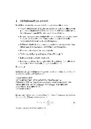
DETERMINANTS OF VECTORS AND MATRICESContents1 Some words about linear algebra 41.1 Linear functions (or maps) . . . . . . . . . . . . . . . . . . . . . . . . . . . . 41.2 Linear spaces . . . . . . . . . . . . . . . . . . . . . . . . . . . . . . . . . . . 41.3 Examples of linear maps . . . . . . . . . . . . . . . . . . . . . . . . . . . . . 51.4 Dimension and basis . . . . . . . . . . . . . . . . . . . . . . . . . . . . . . . 72 Geometrical meanings of determinants 92.1 Determinant of a square matrix . . . . . . . . . . . . . . . . . . . . . . . . . . 92.2 Area of a parallelogram . . . . . . . . . . . . . . . . . . . . . . . . . . . . . . 92.3 Computation of det ( ⃗i,⃗j) (⃗u, ⃗v) when ⃗u = a ⃗i + c⃗j and ⃗v = b⃗i + d⃗j . . . . . . . . 102.4 Determinant of a linear function from E to E . . . . . . . . . . . . . . . . . . 122.5 Two interpretations of the 2 × 2 matrix determinant . . . . . . . . . . . . . . . 122.6 Back to the linear system . . . . . . . . . . . . . . . . . . . . . . . . . . . . . 132.7 Order 3 . . . . . . . . . . . . . . . . . . . . . . . . . . . . . . . . . . . . . . 142.8 Oriented volume of a parallelepiped constructed on 3 vectors . . . . . . . . . . 142.9 Solving a system of 3 linear equations in 3 unknowns . . . . . . . . . . . . . . 163 How to compute determinants of matrices 173.1 One inductive rule . . . . . . . . . . . . . . . . . . . . . . . . . . . . . . . . . 173.2 Main properties of determinants . . . . . . . . . . . . . . . . . . . . . . . . . 183.3 Examples . . . . . . . . . . . . . . . . . . . . . . . . . . . . . . . . . . . . . 194 Definitions and proofs 224.1 Determinant of vectors with respect to a basis . . . . . . . . . . . . . . . . . . 224.2 Determinant of a linear map from E to E . . . . . . . . . . . . . . . . . . . . 244.3 Determinant of a square matrix . . . . . . . . . . . . . . . . . . . . . . . . . . 254.4 A beautiful formula . . . . . . . . . . . . . . . . . . . . . . . . . . . . . . . . 274.5 Linear systems . . . . . . . . . . . . . . . . . . . . . . . . . . . . . . . . . . 27

1 Some words about linear algebra1.1 Linear functions (or maps)A map f : E → F , from a set E to a set F is said to be linear if for any ⃗u and ⃗v in E:f(⃗u + ⃗v) = f(⃗u) + f(⃗v)But then we must also have f(⃗u + ⃗u) = f(⃗u) + f(⃗u) or f(2⃗u) = 2f(⃗u) and in the same wayand so on.f(3⃗u) = f(⃗u + 2⃗u) = f(⃗u) + f(2⃗u) = f(⃗u) + 2f(⃗u) = 3f(⃗u),Also, since 1⃗u + 1 ⃗u = ⃗u, we have2 2f( 1⃗u) + 2 f(1⃗u) = 2 f(1⃗u + 1 ⃗u) = f(⃗u)2 2or 2f( 1 2 ⃗u) = f(⃗u) or even better f(1 2 ⃗u) = 1 2 f(⃗u).In that way we get for any rational number p q the relation f(p q ⃗u) = p q f(⃗u).Since every real number λ is a limit of rational numbers, we get the general rulef(λ⃗u) = λf(⃗u).Now we have a better definition of a linear map or function:A function f : E → F is linear if for any ⃗u and ⃗v in E and any real λ:{ f(⃗u + ⃗v) = f(⃗u) + f(⃗v)f(λ⃗u) = λf(⃗u)1.2 Linear spacesOur previous definition of a linear map or function is not yet quite good since we cannot be surethat the addition and the multiplication by a real number have any meaning in the sets E andF . We have to assume that these operations have meaning in the sets E and F , that is to saywe must have a specific structure on these sets. The structure we need is called ”linear space”.More precisely:Definition 1.2.1 A set E is called a linear space or a vector space (the elements of E will becalled elements or vectors), if there are two operations defined on E:the addition + such that:∀ ⃗u, ⃗v and ⃗w: (⃗u + ⃗v) + ⃗w = ⃗u + (⃗v + ⃗w)∃ ⃗0 such that ∀ ⃗u: ⃗u + ⃗0 = ⃗u∀ ⃗u, ∃ an opposite −⃗u such that ⃗u + (−⃗u) = ⃗0∀ ⃗u and ⃗v: ⃗u + ⃗v = ⃗v + ⃗uthe multiplication of a vector by a real number is such that for any vectors ⃗u and ⃗v and for anyreal numbers λ and µ:

1 SOME WORDS ABOUT LINEAR ALGEBRA 51⃗u = ⃗u and 0⃗u = ⃗0 and (−1)⃗u = −⃗uλ(⃗u + ⃗v) = λ⃗u + λ⃗v(λ + µ)⃗u = λ⃗u + µ⃗uλ(µ⃗u) = (λµ)⃗uExample 1.2.2 n = 0 A set with only the null vector ⃗0 is a vector space if we put the rules⃗0 + ⃗0 = ⃗0 and λ⃗0 = ⃗0.Example 1.2.3multiplication.Example 1.2.4n = 1 The set of real numbers is a vector space with the usual addition andn = 2 The set of matrices with 1 column and 2 rows{( )∣a ∣∣∣R 2×1 = M 2,1 (R) = a, c ∈ R}cbecomes a vector space if we define addition and multiplication by a real number in the following”natural” way: for any two vectors in R 2×1 :( ) ( ( )a b a + b+ := ,c d)c + dand for any vector in R 2×1 and for any real number λ:( ) ( )a λaλ := .c λcThe nul vector is then( 0 ⃗0 := .0)Example 1.2.5n The set R n or M n,1 (R) is a vector space.Example 1.2.6 For any positive integers m and n, the set of matrices R m×n = M n,m (R) withn rows and m columns is a vector space.Example 1.2.7 The set of all real functions defined on R is a vector space iff + g is the function x ↦→ f(x) + g(x) andλf is the function x ↦→ λf(x).1.3 Examples of linear mapsa) f : R → RProposition 1.3.1 A function f from R to R is linear if and only if there is a real number asuch that for any real number u we have:f(u) = au

1 SOME WORDS ABOUT LINEAR ALGEBRA 6Proof. If there is such an a, we havef(u + v) = a(u + v) = au + av = f(u) + f(v),f(λu) = a(λu) = (aλ)u = (λa)u = λ(au) = λf(u).Conversely, suppose f is linear. Since u = 1u = u1, we get f(u) = f(u1) = uf(1) = f(1)u.Let us put a := f(1), we have for any u in R: f(u) = au. ✷b) f : R 2×1 → R 2×1Proposition 1.3.2 A function f from R 2×1 to R 2×1 is linear if and only if there is a 2 by 2matrix A such that for any vector ⃗u we have:f(⃗u) = A⃗u.Proof. First suppose there is such a matrix A. Let us write explicitly A and two vectors ⃗u and⃗v as( ) ( ) ( )a b u1 v1A = , ⃗u = , ⃗v = .c d u 2 v 2Then we have( ) (u1 a bf(⃗u) = f =u 2 c d)(u1) ( ) au1 + bu=2.u 2 cu 1 + du 2We can check that f(⃗u + ⃗v) = f(⃗u) + f(⃗v) explicitly by computing both sides of that equality:(( ) ( )) ( ) ( ) ( )u1 v1 u1 +vf(⃗u+⃗v) = f + = f 1 a(u1 +v=1 )+b(u 2 +v 2 ) au1 +bu=2 +av 1 +bv 2u 2 v 2 u 2 +v 2 c(u 1 +v 1 )+d(u 2 +v 2 ) cu 1 +du 2 +cv 1 +dv 2and on the other hand:f(⃗u)+f(⃗v) = f(u1u 2)+f(v1) ( ) ( ) ( )au1 +bu=2 av1 +bv+2 au1 +bu=2 +av 1 +bv 2v 2 cu 1 +du 2 cv 1 +dv 2 cu 1 +du 2 +cv 1 +dv 2We have also to check that for any real λ and any vector ⃗u, we have f(λ⃗u) = λf(⃗u): the leftside of the equality is in fact( ( )) ( ) ( ) ( )u1 λu1 aλu1 +bλuf(λ⃗u) = f λ = f =2 λ(au1 +bu=2 ),u 2 λu 2 cλu 1 +dλu 2 λ(cu 1 +du 2 )and the right hand side is:λf(⃗u) = λf(u1u 2)= λ( ) au1 +bu 2=cu 1 +du 2( )λ(au1 +bu 2 ),λ(cu 1 +du 2 )Conversely, if f is linear, let us define( ) ( a 1:= f ,c 0)( ( b 0:= f .d)1)Then we can write for any vector ⃗u:( ( ) ( )u1 1 0⃗u =)= uu 1 + u2 0 2 ,1

1 SOME WORDS ABOUT LINEAR ALGEBRA 7and thus by linearity( ( ) ( )) ( ( )) ( ( ))1 0 1 0f(⃗u) = f u 1 + u0 2 = f u11 + f u021( ) ( ) ( ) ( ) ( )a b u1 a u2 b u1 a+u= u 1 + uc 2 = + =2 b=d u 1 c u 2 d u 1 c+u 2 d✷( 1= u 1 f0)( ) au1 +bu 2=cu 1 +du 2( 0+ u 2 f1)( a bcd)(u1u 2)c) f : R 2×1 → RProposition 1.3.3 A function f from R 2×1 to R is linear if and only if there is a 1 by 2 matrix(a b) such that for any vector ⃗u we have:f(⃗u) = ( ab ) ⃗uProof. Left as an exercise. ✷1.4 Dimension and basisa) Affine plane versus vector planeA usual plane such as the blackboard or a sheet of paper gives the image of an affine plane inwhich all the elements, called points, play the same role. To get a vector plane we need to haveone element selected. That element will be the null vector ⃗0. In a vector plane the elements arecalled vectors: we can add them using the parallelogram rule. We can also multiply a vector bya number.From now on, we will only consider the vector plane. Two vectors ⃗u and ⃗v are called collinearor parallel if ⃗v = λ⃗u for some real λ or ⃗u = µ⃗v for some real µ.Notice that ⃗0 is collinear to any vector.b) BasisTo be able to compute anything we need real numbers. To specify every vector we have tochoose two vectors which are not collinear, let us call them ⃗i and ⃗j. Now any vector ⃗u canbe written as ⃗u = u 1⃗i + u 2⃗j and the couple of numbers (u 1 , u 2 ) is unique: we say that (⃗i,⃗j)is a basis of the vector plane. Once we have a basis of the vector plane, we have a bijectionpreserving the operations between the vector plane and R 2 .( ) aa⃗i + c⃗j ←→cTherefore the vector plane is often identified with R 2 .Since a basis has exactly 2 vectors we say that the dimension of the space is 2, dim = 2.

1 SOME WORDS ABOUT LINEAR ALGEBRA 8c) Matrix associated to a linear map from the vector plane into itselfLet L be a linear map from the vector plane into the vector plane and suppose we have chosena basis (⃗i,⃗j). The relation ⃗v = L(⃗u) may be writtenv 1⃗i + v 2⃗j = L(u 1⃗i + u 2⃗j).Suppose L(⃗i) = a⃗i + c⃗j and L(⃗j) = b⃗i + d⃗j, then:v 1⃗i + v 2⃗j = L(u 1⃗i + u 2⃗j) = u 1 L(⃗i) + u 2 L(⃗j)= u 1 (a⃗i + c⃗j) + u 2 (b⃗i + d⃗j) = (au 1 + bu 2 )⃗i + (cu 1 + du 2 )⃗jor {v1 = au 1 + bu 2or even better:We say that the matrix(v1v 2 = cu 1 + du 2) ( a b=v 2 c d)(u1( ) a bA :=c du 2)is associated to the linear map L relatively to the basis (⃗i,⃗j). If we change the basis we getanother matrix A ′ . Then there is an invertible 2 × 2 matrix P such that A and A ′ are related bythe equality A ′ = P −1 AP .d) GeneralizationLet E be a vector space. A sequence of vectors (e 1 , e 2 , . . . , e n ) is a basis if every vector u in Ecan be written in one and only one way as:u = u 1 e 1 + u 2 e 2 + . . . + u n e n .Since a basis has exactly n vectors we say that the dimension of the space is n.For every linear map f : E → E there is one square matrix of order n associated to f relativelyto the basis (e 1 , e 2 , . . . , e n ). If one changes the basis, the matrix is changed following the ruleA ′ = P −1 AP .

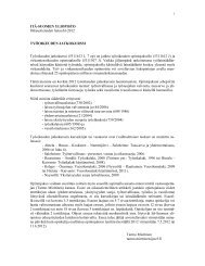
2 Geometrical meanings of determinants2.1 Determinant of a square matrixFor 2×2 matrices ∣ ∣∣∣ a bc d∣ := ad − bc.The system of 2 linear equations in 2 unknowns (x, y){ ax + by = pcx + dy = qhas a unique solution if and only if ad − bc ≠ 0, and the solution is then⎧⎪⎨pd − bqx =ad bcaq − pc⎪⎩ y =ad − bc2.2 Area of a parallelogramLet E be a 2-dimensional vector space with basis (⃗i,⃗j). We choose as unit area the area of theparallelogram constructed on⃗i and ⃗j, that is the parallelogram OP SQ such that−→OP =⃗i,−→OS =⃗i + ⃗jand−→OQ = ⃗j.QjS0 iPProblem 2.2.1 Let ⃗u and ⃗v be two vectors⃗u = a⃗i + c⃗j and ⃗v = b⃗i + d⃗j.What is the area ∆ of the parallelogram constructed on ⃗u and ⃗v?To find ∆ we need 3 rules:Rule 1. If ⃗u is parallel to⃗i and ⃗v parallel to ⃗j, that is⃗u = a⃗i and ⃗v = d⃗jthen ∆ = ad.

2 GEOMETRICAL MEANINGS OF DETERMINANTS 10v = 3ju+vj∆ = 60iu = 2iRule 2 (Euclid, about 300 BC). The area of a parallelogram does not change when you let oneside glide on the line on which it is lyingD C D’ C’DC = D’C’ = ABArea (ABCD) = Area (ABC’D’)ABRule 3. The area is positive if you have to turn in the same direction (to the left or to the right) tomove from ⃗u to ⃗v as from⃗i to ⃗j. The area is negative if you have to turn in opposite directions.Thus the rule 1 is valid even if a and/or d are negative numbers.Definition 2.2.2 The oriented area ∆ is called the determinant of ⃗u and ⃗v with respect to thebasis (⃗i,⃗j) and denoted by∆ = det(⃗u, ⃗v).(⃗i,⃗j)2.3 Computation of det ( ⃗i,⃗j) (⃗u, ⃗v) when ⃗u = a ⃗i + c⃗j and ⃗v = b⃗i + d⃗jdvd - bc ajcui b a

2 GEOMETRICAL MEANINGS OF DETERMINANTS 11First, we use rule 2:det(⃗i,⃗j)(⃗u, ⃗v) = det(⃗u, ⃗v − b a ⃗u)(⃗i,⃗j)(= det(⃗i,⃗j)a⃗i + c⃗j, (d − bc a ) ⃗jUsing rule 2 once again (for the other side) we get((⃗u, ⃗v) = det a⃗i, (d − bc a ) ⃗jThen the rule 1 gives usdet(⃗i,⃗j)det(⃗i,⃗j)(⃗i,⃗j)).).(⃗u, ⃗v) = a (d − bc a ) det (⃗i,⃗j) = ad − bc.The next Theorem gives a characterisation of the function det ( ⃗i,⃗j) : E × E → R.(⃗i,⃗j)Theorem 2.3.1 The function det ( ⃗i,⃗j) : E × E → R,is the only function from E × E to R such that(a⃗i + c⃗j, b⃗i + d⃗j) ↦−→ ad − bc(i) For all ⃗u ∈ E the function det ( ⃗i,⃗j)(⃗u, ·) : E → R is linear.For all ⃗v ∈ E the function det ( ⃗i,⃗j)(·, ⃗v) : E → R is linear.(ii) For all ⃗u ∈ E holds det ( ⃗i,⃗j)(⃗u, ⃗u) = 0.(iii) det ( ⃗i,⃗j) ( ⃗i,⃗j) = 1.The (i) means that for any vectors ⃗u, ⃗v, ⃗u ′ and ⃗v ′ , and any numbers λ and µ, we havedet(⃗i,⃗j)det(⃗i,⃗j)(⃗u, λ⃗v + µ⃗v ′ ) = λ det(⃗u,⃗v) + µ det(⃗u,⃗v ′ )(⃗i,⃗j)(⃗i,⃗j)(λ⃗u + µ⃗u ′ , ⃗v) = λ det(⃗u,⃗v) + µ det(⃗u ′ , ⃗v).Proof. To prove the existence we just have to check that (i), (ii) and (iii) are true. To proveunicity, we proceed in two steps.Step 1. For any function ϕ : E × E → R such that (i) holds we have for any vectors ⃗u and ⃗v:If ϕ is such that (ii) holds, we getso thatStep 2. Using (i), we get(⃗i,⃗j)(⃗i,⃗j)ϕ(⃗u + ⃗v, ⃗u + ⃗v) = ϕ(⃗u, ⃗u) + ϕ(⃗u, ⃗v) + ϕ(⃗v, ⃗u) + ϕ(⃗v, ⃗v).0 = 0 + ϕ(⃗u, ⃗v) + ϕ(⃗v, ⃗u) + 0ϕ(⃗v, ⃗u) = −ϕ(⃗u,⃗v). (1)ϕ(a⃗i + c⃗j, b⃗i + d⃗j) = ab ϕ(⃗i,⃗i) + ad ϕ(⃗i,⃗j) + bc ϕ(⃗j,⃗i) + cd ϕ(⃗j,⃗j).From (ii) and (1) we deduceand (iii) shows that ϕ = det ( ⃗i,⃗j) . ✷ϕ(a⃗i + c⃗j, b⃗i + d⃗j) = (ad − bc)ϕ(⃗i,⃗j),

2 GEOMETRICAL MEANINGS OF DETERMINANTS 122.4 Determinant of a linear function from E to ELemma 2.4.1 Let E be a 2-dimensional vector space with a basis (⃗i,⃗j) and let f : E → E bea linear function. Then there is a number δ j such that:∀ ⃗u ∈ E, ∀ ⃗v ∈ Edet(⃗i,⃗j)(f(⃗u), f(⃗v)) = δ j det(⃗u, ⃗v). (2)(⃗i,⃗j)Proof. Let ϕ : E × E → R be the mapping(⃗u, ⃗v) ↦−→ ϕ(⃗u,⃗v) = det (f(⃗u), f(⃗v)).(⃗i,⃗j)It easy to check that ϕ satisfies (i) and (ii) of Theorem 2.3.1. By the same reasoning as above,we get:ϕ(a⃗i + c⃗j, b⃗i + d⃗j) = (ad − bc) ϕ(⃗i,⃗j).Thusis such that (2) holds. ✷δ f := ϕ(⃗i,⃗j) = det (f(⃗i), f(⃗j))(⃗i,⃗j)Interpretation of the LemmaApplying f we transform a parallelogram constructed on any two vectors ⃗u and ⃗v into a parallelogramconstructed on f(⃗u) and f(⃗v). The lemma means that the ratio between the areas ofthese parallelograms does not depend on the choice of ⃗u and ⃗v, but only on f. The ratio may bewrittenδ f = det (f(⃗u), f(⃗v))(⃗u,⃗v)for any couple of independent vectors ⃗u and ⃗v. This justifies the following definition.Definition 2.4.2 Let f : E → E be linear. The determinant of f, denoted det f or det(f), isthe number independent of the choice of the basis (⃗i,⃗j)det f := det (f(⃗i), f(⃗j)).(⃗i,⃗j)Remark 2.4.3 Since det f is the coefficient which multiplies the areas when we use the transformationf, we havedet(g ◦ f) = det g · det f.2.5 Two interpretations of the 2 × 2 matrix determinantInterpretation 1Let us denote( ) ( ( a b1 0A = , ⃗ec d1 := , ⃗e0)2 :=1)Then the determinant with respect to the standard basis (⃗e 1 , ⃗e 2 ) of the two column vectors of Ahas the same value as the determinant of the matrix A, provided we preserve their order:det A =∣ a b(( ) ( a bc d ∣ = det ,(⃗e 1 ,e 2 ) c d))

2 GEOMETRICAL MEANINGS OF DETERMINANTS 13Interpretation 2Let (⃗i,⃗j) be a basis of a vector-space E. The matrix A is associated to the linear functionf : E → E is defined byf(⃗i) = a⃗i + c⃗j and f(⃗j) = b⃗i + d⃗j.Thendet A = det f.Remark 2.5.1 The relation det(g ◦ f) = det g · det f will becomedet(BA) = det B · det Afor all 2×2 matrices B and A.We may check this formula explicitly. Let( ) a bA =c d( ) a′band B =′c ′ d ′ .Thenand( )aBA =′ a + b ′ c a ′ b + b ′ dc ′ a + d ′ c c ′ b + d ′ ddet(BA) = (a ′ a + b ′ c)(c ′ b + d ′ d) − (a ′ b + b ′ d)(c ′ a + d ′ c)= a ′ d ′ ad + b ′ c ′ bc − a ′ d ′ bc − b ′ c ′ ad= (a ′ d ′ − b ′ c ′ )(ad − bc) = det B · det A.Remark 2.5.2 If we change basis, the matrix associated with f is changed from A to P −1 AP ,where P is an invertible (i.e. regular) matrix and P −1 is the inverse of P . We have as we expectdet(P −1 AP ) = det Asince the two numbers are equal to det f. We can check:det(P −1 AP ) = det P −1 · det A · det P= det P −1 · det P · det A= det(P −1 P ) · det A= det I · det A= det A.2.6 Back to the linear systemWe write the system { ax + by = pcx + dy = qas a linear combinationP = xU + yV,

2 GEOMETRICAL MEANINGS OF DETERMINANTS 14where( ) ( )p aP = , U =q c( band V =d)To find x and y, just notice thatanddet (P, V ) = det (xU + yV, V ) = x det (U, V )(⃗e 1 ,⃗e 2 ) (⃗e 1 ,⃗e 2 ) (⃗e 1 ,⃗e 2 )det (U, P ) = y det (U, V )(⃗e 1 ,⃗e 2 ) (⃗e 1 ,⃗e 2 )We find the unique solution, whenever det (⃗e1 ,⃗e 2 )(U, V ) = ad − bc ≠ 0, is accordance withCramer’s rule:∣ p bq d ∣∣ a pc q ∣x =∣ a band y =c d ∣∣ a bc d ∣2.7 Order 3Determinant of a square matrix of order 3We define (or remember that)∣ a 11 a 12 a 13 ∣∣∣∣∣ a 21 a 22 a 23 := a 11 a 22 a 33 + a 12 a 23 a 31 + a 13 a 21 a 32 − a 13 a 22 a 31 − a 11 a 23 a 32 − a 12 a 21 a 33∣ a 31 a 32 a 33Remark 2.7.1 The Sarrus’ rule is a practical rule for computing determinants of order 3. Use+ sign in front of the products of factors on a parallel to the main diagonal of the matrix and −sign for parallels to the other diagonal:+−a 31 a 32 a 33 a 31 a 32a 11 a 12 a 13 a 11 a 12. .. . .. . ..a 21 a 22 a 23 a 21 a 22. .. . .. . ..a 11 a 12 a 13 a 11 a 12. .. . .. . ..a 21 a 22 a 23 a 21 a 22. .. . .. . ..a 31 a 32 a 33 a 31 a 322.8 Oriented volume of a parallelepiped constructed on 3 vectorsSuppose that E is a vector space with base (⃗i,⃗j, ⃗ k) and let ⃗u, ⃗v and ⃗w be vectors in E. Theoriented volume of the parallelepiped constructed on these vectors ⃗u, ⃗v and ⃗w is denoteddet ( ⃗i,⃗j, ⃗ k)(⃗u, ⃗v, ⃗w) if the unit is the volume constructed on the basis.We may accept the following rules:Rule 1. det ( ⃗i,⃗j, ⃗ k) (a ⃗i, b⃗j, c ⃗ k) = abc.

2 GEOMETRICAL MEANINGS OF DETERMINANTS 15Rule 2. The volume of the parallelepiped is not modified when one side is gliding in the planein which it lies:det (⃗u, ⃗v, ⃗w + λ⃗u + µ⃗v) = det (⃗u, ⃗v, ⃗w).(⃗i,⃗j, ⃗ k)(⃗i,⃗j, ⃗ k)Rule 3. The volume is positive (resp. negative) if (⃗u, ⃗v, ⃗w) has the same (resp. opposite) orientationas the basis (⃗i,⃗j, ⃗ k).Computed value of the volume isdet(⃗i,⃗j, ⃗ k)∣ ∣ ∣∣∣∣∣ a 11 a 12 a 13 ∣∣∣∣∣(a 11⃗i + a 21⃗j + a 31⃗ k, a12 ⃗i + a 22⃗j + a 32⃗ k, a13 ⃗i + a 23⃗j + a 33⃗ k) = a 21 a 22 a 23a 31 a 32 a 33Characterisation of the function det ( ⃗i,⃗j, ⃗ k) : E3 → RTheorem 2.8.1 The function det ( ⃗i,⃗j, ⃗ k)from E 3 to R such that: (⃗u, ⃗v, ⃗w) ↦−→ det (⃗i,⃗j, ⃗ k)(⃗u, ⃗v, ⃗w) is the only function(i) the functions det ( ⃗i,⃗j, ⃗ k) (·, ⃗v, ⃗w), det (⃗i,⃗j, ⃗ k) (⃗u, ·, ⃗w) and det (⃗i,⃗j, ⃗ k)(⃗u,⃗v, ·) are linear(ii) det ( ⃗i,⃗j, ⃗ k) (⃗u, ⃗u, ⃗w) = 0, det (⃗i,⃗j, ⃗ k) (⃗u, ⃗v, ⃗u) = 0 and det (⃗i,⃗j, ⃗ k)(⃗u, ⃗v, ⃗v) = 0(iii) det ( ⃗i,⃗j, ⃗ k) ( ⃗i,⃗j, ⃗ k) = 1.Determinant of a linear function f from E to ETheorem 2.8.2 Let E be a 3-dimensional vector space and let f : E → E be linear. Thenumberdet f := det (f(⃗i), f(⃗j), f( ⃗ k))(⃗i,⃗j, ⃗ k)is independent of the choice of the basis (⃗i,⃗j, ⃗ k).Definition 2.8.3 The base invariant number det f is called the determinant of the linear functionf : E → E (see Theorem 2.8.2).Remark 2.8.4 det f is the multiplication coefficient of volumes when you apply the transformationf, thusdet(g ◦ f) = det g · det f.If⎛⎞⎛ ⎞ ⎛ ⎞ ⎛ ⎞a 11 a 12 a 13100A = ⎝a 21 a 22 a 23⎠, and ⃗e 1 := ⎝0⎠, ⃗e 2 := ⎝1⎠, ⃗e 3 := ⎝0⎠,a 31 a 32 a 33 001you can think of det A asdet A =det(⃗e 1 ,⃗e 3 ,⃗e 3 )⎛⎛⎞ ⎛ ⎞ ⎛ ⎞⎞a 11 a 12 a 13⎝⎝a 21⎠, ⎝ a 22⎠, ⎝ a 23⎠⎠a 31 a 32 a 33or as det A = det f, if f is a linear function whose associated matrix is A with respect to somebasis.

2 GEOMETRICAL MEANINGS OF DETERMINANTS 162.9 Solving a system of 3 linear equations in 3 unknownsFollowing the idea of Subsection 2.6, let us again write the system⎧⎨ a 11 x 1 + a 12 x 2 + a 13 x 3 = b 1a 21 x 1 + a 22 x 2 + a 23 x 3 = b 2⎩a 31 x 1 + a 32 x 2 + a 33 x 3 = b 3as a linear combination of the columns:whereNotice thatB = x 1 V 1 + x 2 V 2 + x 3 V 3 ,⎛ ⎞ ⎛ ⎞ ⎛ ⎞⎛ ⎞b 1a 11a 12a 13B = ⎝b 2⎠, V 1 = ⎝a 21⎠, V 2 = ⎝a 22⎠ and V 3 = ⎝a 23⎠.b 3 a 31 a 32 a 33det(⃗e 1 ,⃗e 3 ,⃗e 3 ) (B, V 2, V 3 ) = x 1det (V 1, V 2 , V 3 ).(⃗e 1 ,⃗e 3 ,⃗e 3 )Thus, if V 1 , V 2 and V 3 are linearly independent we again get Cramer’s rule∣ ∣ b 1 a 12 a 13 ∣∣∣∣∣a 11 b 1 a 13 ∣∣∣∣∣b 2 a 22 a 23a 21 b 2 a 23∣ b 3 a 32 a 33∣ a 31 b 3 a 33∣x 1 =∣, x a 11 a 12 a 13 ∣∣∣∣∣ 2 =∣, x a 11 a 12 a 13 ∣∣∣∣∣ 3 =a 21 a 22 a 23a 21 a 22 a 23∣ a 31 a 32 a 33∣ a 31 a 32 a 33∣∣a 11 a 12 b 1 ∣∣∣∣∣a 21 a 22 b 2a 31 a 32 b 3∣a 11 a 12 a 13 ∣∣∣∣∣a 21 a 22 a 23a 31 a 32 a 33

3 How to compute determinants of matrices3.1 One inductive ruleDefinition 3.1.1 Let A be a square matrix of order n ≥ 2. We denote by M A ij and call minormatrix of A indexed by i and j when 1 ≤ i ≤ n and 1 ≤ j ≤ n, the matrix obtained when yousupress the i-row and the j-column of A.If A = (a ij ) n×n , then⎛⎞a 11 . . . a 1,j−1 a 1,j+1 . . . a 1n.. .Mij A a= i−1,1 . . . a i−1,j−1 a i−1,j+1 . . . a i−1,na i+1,1 . . . a i+1,j−1 a i+1,j+1 . . . a i+1,n⎜⎟⎝ .. .. ⎠a n,1 . . . a n,j−1 a n,j+1 . . . a nnRule. Let A be a square matrix A = (a ij ) n×n .1. If n = 1, then det(a 11 ) := a 11 .2. If n ≥ 2, the cofactor A ij of the element a ij of A isA ij := (−1) i+j det (M A ij ).The determinant of A is a number det A such that for any row r and any column kdet A =n∑a rj A rj =j=1n∑a ik A ik .i=1Remark 3.1.2 If we use the first formula, we say that we are developing the determinant of Aalong the row r. If we use the second, we develop along the column k.Remark 3.1.3 To remember the sign to use, you just have to think of the game chess:⎛⎞+ − + − + . . .− + − + −+ − + − +− + − + −⎜⎝+ − + − + ⎟⎠. +Example 3.1.4 Let( )a11 aA =12.a 21 a 22The cofactors are A 11 = a 22 , A 12 = −a 21 , A 21 = −a 12 and A 22 = a 11 . There are fourpossibilities for developing det A, giving happily the same result.Developing along the first row:det A = a 11 A 11 + a 12 A 12 = a 11 a 22 − a 12 a 21 ,

3 HOW TO COMPUTE DETERMINANTS OF MATRICES 18along the second row:and along the columuns:det A = a 21 A 21 + a 22 A 22 = −a 21 a 12 + a 22 a 11 ,det A = a 11 A 11 + a 21 A 21 = a 11 a 22 − a 21 a 12det A = a 12 A 12 + a 22 A 22 = −a 12 a 21 + a 22 a 11 .Example 3.1.5 Developing along the first row:3 0 1∣ ∣ ∣ ∣∣∣ 2 −1 0∣ −4 1 2 ∣ = 3 −1 0∣∣∣ 1 2 ∣ − 0 2 0∣∣∣ −4 2 ∣ + 1 2 −1−4 1 ∣ = 3(−2) + (−2) = −8.Example 3.1.6 Compute det A for⎛⎞2 −1 0 3A = ⎜ 1 3 0 1⎟⎝−1 2 −1 0⎠ .0 −4 1 2Let us develop it along the third column (why?). We get2 −1 0 3∣ 1 3 0 12 −1 3∣∣∣∣∣ 2 −1 3−1 2 −1 0= (−1)1 3 1∣∣ 0 −4 1 2 ∣ 0 −4 2 ∣ − 1 1 3 1= −10 − 12 = −22.−1 2 0 ∣3.2 Main properties of determinantsLet A = (a ij ) be a n × n square matrix.1. det(AB) = det A · det B.2. det(λI) = λ n , det(λA) = λ n det A for λ ∈ R (order of A is n).3. If A is regular, then det(A −1 ) = (det A) −1 .4. det A T = det A.5. For triangular (and diagonal) matrices, the determinant is the product of the elements onthe main diagonal∣ ∣ λ 1 ∣∣∣∣∣∣∣∣∣∣ λ 1 ∣∣∣∣∣∣∣∣∣∣ λ 2 ∗λ 2 O. ..=. ..= λ 1 λ 2 . . . λ n .O λ n−1 ∗ λ n−1∣λ n∣λ n6a. If all the elements of a row are zero, then the determinant is zero.

3 HOW TO COMPUTE DETERMINANTS OF MATRICES 196b. If all the elements of a column are zero, then the determinant is zero.7a. If two rows are proportional, the determinant is zero.7b. If two columns are proportional, the determinant is zero.8a. If a row is a linear combination of the others, then the determinant is zero.8b. If a column is a linear combination of the others, then the determinant is zero.9. Let B be the matrix deduced from A by(i) permutation of two rows (resp. columns), then det B = − det A.(ii) multiplication of all the elements of a row (resp. column) by a number k,then det B = k det B.(iii) addition of the multiple of a line (resp, a columns) to an other, thendet B = det A.10. If P is a regular matrix, thendet(P −1 AP ) = det A.3.3 ExamplesExample 3.3.1a a − 1 a + 2a + 2 a a − 1∣ a − 1 a + 2 a ∣Example 3.3.2 Let’s computeD a,b =∣3a + 1 a − 1 a + 2=3a + 1 a a − 1add col 2 and 3 to col 1∣ 3a + 1 a + 2 a ∣ 1 a − 1 a + 2= (3a + 1)1 a a − 1by property 9 (ii)∣ 1 a + 2 a ∣ 1 a − 1 a + 2∣ ∣∣∣= (3a + 1)0 1 −3∣ 0 3 −2 ∣ = (3a + 1) 1 −33 −2 ∣ = 7(3a + 1).1 + a 1 1 11 1 − a 1 11 1 1 + b 11 1 1 1 − bSubtract the second column from the first and after that first row from the result:a 1 1 1a 1 1 1D a,b =a 1 − a 1 10 1 1 + b 1=0 −a 0 00 1 1 + b 1.∣ 0 1 1 1 − b ∣ ∣ 0 1 1 1 − b ∣Develop along the first column, and then again:−a 0 0∣ ∣∣∣D a,b = a1 1 + b 1∣ 1 1 1 − b ∣ = a(−a) 1 + b 11 1 − b ∣ = −a2 (−b 2 ) = a 2 b 2 ..∣

3 HOW TO COMPUTE DETERMINANTS OF MATRICES 20Example 3.3.3 Compute the determinant of order n1 1 1 · · · 1 1−1 0 1 · · · 1 1−1 −1 0 · · · 1 1D n =. . . . .. .. .−1 −1 −1 · · · 0 1∣ −1 −1 −1 · · · −1 0 ∣Add the first row to all the others, you get a triangular matrix, with only 1’s on the diagonal.Thus D n = 1.Example 3.3.4 The Vandermonde determinant.Let x 1 , x 2 ,. . ., x n be n real numbers. Compute the polynomial1 x 1 x 2 1 . . . x n−111 x 2 x 2 2 . . . x n−12∆(x 1 , x 2 , . . . , x n ) =. . ... . . .∣ 1 x n x 2 n . . . x n−1 ∣nSince ∆ = 0, if x i = x j , we can factorize by x i −x j . It is easy to see that ∆ is homogeneous ofdegreen(n − 1)0 + 1 + 2 + . . . + (n − 1) = .2Thus∆ = k ∏ i − x j )i>j(xwhere k is a constant. We determine k by considering the coefficient of x 2 x 2 3 . . . xnn−1is 1. So finally we get∆ = ∏ i − x j ).i>j(xwhichExample 3.3.5 The Hilbert determinant.Let us computeH n =.∣Substract the last row from the others:n−1nn−22nn−33nH n =.1(n−1)n∣1n1112131nn−12(n+1)n−23(n+1)n−34(n+1)1n(n+1)1n+11213141n+111. . . 3 n11. . . 4 n+11.5. .. .11. . . ∣n+2 2n−1n−1n−1. . .3(n+2) n(2n−1)n−2n−2. . .4(n+2) (n+1)(2n−1)n−35(n+2).. .. .11. . .(n+1)(n+2) (2n−2)(2n−1)11. . .n+2 2n−1∣

3 HOW TO COMPUTE DETERMINANTS OF MATRICES 21=(n − 1)!n(n + 1) . . . (2n − 1)∣1 111 . . . 2 3 n1 1 11. . . 2 3 4 n+11 1 1.3 4 5.... .1 11. . . n n+1 2n−21 1 1 . . . 1∣1n−1Substract the last column from the others:H n ==(n − 1)!(n − 1)!n(n + 1) · · · (2n − 1) n(n + 1) · · · (2n − 2) H n−1n∏ 1 ((j − 1)!) 42j − 1 ((2j − 1)!) 2j=1We get the following numbersH 1 = 1, H 2 = 112 , H 3 = 1180 ·112 = 12160 , H 4 = 12800 ·12160 = 16048000 , . . .We notice that H n becomes very small, even compared to the values of the elements of thematrix; it is very useful for testing numerical methods, because this matrix is very unstable withrespect to the values of its elements.

4 DEFINITIONS AND PROOFS 23Theorem 4.1.5 Let E be a vector space of dimension n and let (e 1 , . . . , e n ) be a basis of E.For any number λ there is a unique function ϕ : E n → R such that:(i) ϕ is multilinear,(ii) ϕ is alternate,(iii) ϕ(e 1 , . . . , e n ) = λ.If for j ∈ {1, . . . , n} we have v j = ∑ ni=1 a ije i , thenϕ(v 1 , v 2 , . . . , v n ) = ϕ(e 1 , e 2 , . . . , e n ) ∑ σ∈ϕ nε σ1 σ 2 ...σ na σ1 1, a σ2 2 . . . a σn n.Proof. Let v j = ∑ ni=1 a ije i for j = 1, 2, . . . , n. Then( n∑ϕ(v 1 , v 2 , . . . , v n ) = ϕ a i1 1 e i1 ,i 1 =1Let us suppose that ϕ is multilinear. Thenϕ(v 1 , v 2 , . . . , v n ) =n∑i 1 =1 i 2 =1n∑. . .n∑a i2 2 e i2 , . . . ,i 2 =1n∑a inn e in).i n=1n∑a i1 1a i2 2 . . . a in nϕ(e i1 , e i2 , . . . , e in ).i n =1Let us suppose that ϕ is also alternate; then ϕ(e i1 , e i2 , . . . , e in ) = 0 unless there isσ ∈ S n such that i 1 = σ 1 , i 2 = σ 2 , . . . , i n = σ n . And sinceϕ(e σ1 , e σ2 , . . . , e σn ) = ε σ1 σ 2 ...σ nϕ(e 1 , e 1 , . . . , e n ),we may factorize by ϕ(e 1 , e 2 , . . . , e n ) getting the last formula of the theorem. If we chooseϕ(e 1 , e 2 , . . . , e n ) = λ, the function ϕ is determined. To finish the proof we just have to checkthat the function defined in that way have the properties (i), (ii) and (iii). ✷Definition 4.1.6 The function ϕ such that λ = 1 is denoted det (e1 ,...,e n ) and the image of(v 1 , . . . , v n ) by that function det (e1 ,...,e n )(v 1 , . . . , v n ) is called the determinant of the vectorsv 1 , . . . , v n with respect to the basis (e 1 , . . . , e n ).Remark 4.1.7 We may define the hypervolume in the space E of the generalized parallelepipedconstructed on v 1 , v 2 , . . . v n as det (e1 ,...,e n )(v 1 , . . . , v n ) when we take as unit the hypervolume ofthe generalized parallelepiped constructed on e 1 , . . . , e n .Corollary 4.1.8 If (e 1 , . . . , e n ) is a basis of the n-dimensional vector space E, and if ϕ : E n →R is multilinear and alternate, thenϕ = ϕ(e 1 , . . . , e n )that is to say that for every (u 1 , . . . , u n ) in E n :ϕ(u 1 , . . . , u n ) = ϕ(e 1 , . . . , e n )det ,(e 1 ,...,e n )det (u 1, . . . , u n ).(e 1 ,...,e n )Proof. The assertion follows imediately from the theorem and the definition of det (e1 ,...,e n ). ✷

4 DEFINITIONS AND PROOFS 24Corollary 4.1.9 If (e 1 , . . . , e n ) and (v 1 , . . . , v n ) are two basis of E, thendet (v 1, . . . , v n ) · det (e 1, . . . , e n ) = 1.(e 1 ,...,e n ) (v 1 ,...,v n )Proof. Since (v 1 , . . . , v n ) is a basis, ϕ = det (v1 ,...,v n ) is multilinear and alternate, thus:det (u 1, . . . , u n ) = det (u 1, . . . , u n ) · det (e 1, . . . , e n ).(v 1 ,...,v n ) (e 1 ,...,e n ) (v 1 ,...,v n )For (u 1 , . . . , u n ) = (v 1 , . . . , v n ), we get the expected formula. ✷Corollary 4.1.10 Let (e 1 , . . . , e n ) be a basis of an n-dimensional vector space E. Then: any nvectors v 1 , v 2 , . . ., v n are linearly independent if and only if det (e1 ,...,e n ) (v 1 , . . . , v n ) ≠ 0.Proof. One side with contradiction: If v 1 , v 2 , . . ., v n are linearly dependent, at least one of thevectors is a linear combination of the others, and since det (e1 ...e n ) is multilinear and alternatedet (e1 ,...,e n) (v 1 , . . . , v n ) = 0.On the other hand, if v 1 , v 2 , . . ., v n are linearly independent, they form a basis and thus fromCorollary 4.1.9 we have det (e1 ,...,e n ) (v 1 , . . . , v n ) ≠ 0. ✷4.2 Determinant of a linear map from E to ETheorem and Definition 4.2.1 Let E be a vector space of dimension n and let f : E → E belinear. The number det (e1 ,...,e n ) (f(e 1 ), . . . , f(e n )) is independent of the basis (e 1 , . . . , e n ) of E.This number is called the determinant of f and denoted by det f:det f :=det (f(e 1 ), . . . , f(e n )).(e 1 ,...,e n)Proof. Let (e 1 , . . . , e n ) and (v 1 , . . . , v n ) be two basis of E. We haveFor simplicity, we put det e v := det (e1 ,...,e n )(v 1 , . . . , v n ).Since (e 1 , . . . , e n ) is a basis and the mapping E n → R,det (v 1 , . . . , v n ) ≠ 0. (3)(e 1 ,...,e n )(u 1 , . . . , u n ) ↦−→ det (f(u 1 ), . . . , f(u n )),eis multilinear and alternate, the Corollary 4.1.8 gives: for all (u 1 , . . . , u n ) ∈ E ndet (f(u 1), . . . , f(u n )) = det (f(e 1), . . . , f(e n )) · det (u 1, . . . , u n ).(e 1 ,...,e n ) (e 1 ,...,e n ) (e 1 ,...,e n )And then for (u 1 , . . . , u n ) = (v 1 , . . . , v n ):det (f(v 1), . . . , f(v n )) = det v · det (f(e 1), . . . , f(e n )). (4)(e 1 ,...,e n ) e (e 1 ,...,e n )Since (v 1 , . . . , v n ) is a basis and the mapping E n → R,(u 1 , . . . , u n ) ↦−→ dete (u 1, . . . , u n )

4 DEFINITIONS AND PROOFS 25is multilinear and alternate, the Corollary 4.1.8 gives: for all (u 1 , . . . , u n ) ∈ E ndet (u 1, . . . , u n ) = det v · det (u 1, . . . , u n ).(e 1 ,...,e n) e (v 1 ,...,v n)And thus for (u 1 , . . . , u n ) = (f(v 1 ), . . . , f(v n )) we have:det (f(v 1), . . . , f(v n )) = det v · det (f(v 1), . . . , f(v n )) (5)(e 1 ,...,e n) e (v 1 ,...,v n)From the equations (3), (4) and (5) we get then:✷det (f(e 1), . . . , f(e n )) = det (f(v 1), . . . , f(v n )).(e 1 ,...,e n) (v 1 ,...,v n)Corollary 4.2.2 Let f : E → E be linear. Then det f ≠ 0 if and only if f is bijective.Proof. A linear function f from a linear space of dimension n into a linear space of samedimension, is bijective if and only if it is surjective, that is if and only if the images of basisvectors f(e 1 ), . . . , f(e n ) are linearly independent, or✷det f =det (f(e 1), . . . , f(e n )) ≠ 0.(e 1 ,...,e n )Proposition 4.2.3 If f : E → E and g : E → E are linear, thendet(g ◦ f) = det g · det f.Proof. If f is not bijective, then g ◦ f is not bijective and both sides of the equality are zero.If f is bijective, f(e 1 ), . . . , f(e n ) is a basis for any basis e 1 , . . . , e n and✷det(g ◦ f) = det (g(f(e 1 )), . . . , g(f(e n )))(e 1 ,...,e n)= det (g(f(e 1 )), . . . , g(f(e n ))) · det (f(e 1 ), . . . , f(e n ))(f(e 1 ),...,f(e n))(e 1 ,...,e n)= det g · det f.4.3 Determinant of a square matrixDefinition 4.3.1 Let A be a square matrix of order n. We denote the elements of A by a ij for1 ≤ i ≤ n, 1 ≤ j ≤ n. The determinant of A, denoted by det A, is the numberdet A := ∑ σ∈S nε σ1 σ 2 ...σ na σ1 1a σ2 2 . . . a σnn,where S n is the set of all permutations of {1, 2, 3, . . . , n}.

4 DEFINITIONS AND PROOFS 26Proposition 4.3.2 The determinant of a matrix and the determinant of its column vectors withrespect to the natural basis (e 1 , . . . , e n ) are the same:⎛⎛⎞ ⎛ ⎞ ⎛ ⎞⎞a 11 a 12 a 1na 21det A = det ⎜⎜⎟(e 1 ,...,e n ) ⎝⎝. ⎠ , a 22⎜ ⎟⎝ . ⎠ , . . . , a 2n⎜ ⎟⎟⎝ . ⎠⎠a n1 a n2 a nnProof. A direct consequence of Theorem 4.1.5 and Definition 4.1.6. ✷Proposition 4.3.3 Suppose E is a vector space of dimension n. Let f : E → E be linear and let(e 1 , . . . , e n ) be a basis of E. The matrix A associated with f relatively to the basis (e 1 , . . . , e n )is such that:det A = det f.Proof. The elements a ij are such that f(e j ) = ∑ ni=1 a ije i . Then✷det A =det (f(e 1), . . . , f(e n )) = det f.(e 1 ...e n)Corollary 4.3.4 If A and B are square matrix of order n, thendet(AB) = det A · det B.Proof. Let A be associated with f, and B with g relatively to some basis. Then✷det(BA) = det(g ◦ f) = det g · det f = det B · det A.Proposition 4.3.5 If A is a square matrix thendet A T = det A.Proof. Let us write sgn(σ) := ε σ1 σ 2 ...σ n, when σ ∈ S n . Notice that the function S n → S n ,τ ↦→ τ −1 , is bijective and sgn(τ) = sgn(τ −1 ). Thus:det A = ∑ σ∈S nsgn(σ) a σ1 1 . . . a σn n = ∑ σ∈S nsgn(σ) a 1 σ−11. . . a n σ−1n= ∑ τ∈S nsgn(τ −1 ) a 1 τ1 . . . a n τn = ∑ τ∈S nsgn(τ) a 1 τ1 . . . a n τn = det A T .An alternate proof is to write A = P T Q, with A T = Q T T T P T , where P is a product ofGaussian process matrices with determinant ±1, Q is a permutation matrix with determinant±1 and T triangular. Then✷det A T = det Q T T T P T = det Q T · det T T · det P T= det Q · det T · det P = det P · det T · det Q = det(P T Q) = det A.

4 DEFINITIONS AND PROOFS 274.4 A beautiful formulaDefinition and Proposition 4.4.1 Let A be a square matrix of order n. We denote its elementsby a ij . The minor matrix M A ij is the matrix obtained by supressing the row i and the columnj of the matrix A. The determinant A ij = det(M A ij ) is called the cofactor of the element a ij .The matrix whose element are A ij is the cofactor matrix, and the transposed matrix is called theadjoint matrix of A and denoted by adj A. Thus ( adj A) ij= A ji . Then:A adj A = ( adj A)A = (det A)I.Proof. Since det A = ∑ σ∈S nε σ1 ...σ na 1 σ1 · · · a n σn , we getdet A =n∑i=1a ki A ki = (A( adj A)) kk.If we compute ∑ ni=1 a kiA ji we get the determinant of a matrix with two equal columns and then(A( adj A)) jk= 0 if j ≠ k. Thus the formula. ✷Corollary 4.4.2 The matrix A is invertible (regular) if and only if det A ≠ 0. If det A ≠ 0,then:A −1 = 1 adj A.det AIf det A = 0, A is not invertible, because if it was there would be a matrix B such that AB = I,and then det A · det B = 1, so det A = 0 would be impossible.4.5 Linear systemsTheorem 4.5.1 Let us consider the following vectors and matrices:⎛ ⎞ ⎛ ⎞ ⎛ ⎞a 11 a 12a 1n⎜ ⎟ ⎜ ⎟ ⎜ ⎟V 1 = ⎝ . ⎠, V 2 = ⎝ . ⎠, . . . , V n = ⎝ . ⎠,a n1 a n2 a nn⎛⎞ ⎛ ⎞A := ( a) 11 . . . a 1n b 1⎜⎟ ⎜ ⎟V 1 . . . V n = ⎝ . . ⎠, B = ⎝ . ⎠.a n1 . . . a nn b nThe linear system of n equations in n unknowns x 1 , x 2 , . . ., x n :⎧a 11 x 1 + a 12 x 2 + · · · + a 1n x n = b 1⎪⎨ a 21 x 1 + a 22 x 2 + · · · + a 2n x n = b 2⎪⎩has a unique solution if and only if det A ≠ 0..a n1 x 1 + a n2 x 2 + · · · + a nn x n = b nWhen det A ≠ 0, the solution is given for every x k byx k = det( V 1 . . . V k−1 B V k+1 . . . V n)det A.

4 DEFINITIONS AND PROOFS 28Proof. Let us write the system asB = x 1 V 1 + x 2 V 2 + . . . + x n V n .1) If det A = 0, the vectors V 1 , . . . , V n are linearly dependent and do not generate R n . If Bdoes not belong to the subspace generated by V 1 , . . . , V n , then the system has no solutions. If Bbelongs to that subspace then there are scalars ξ k such thatB = ξ 1 V 1 + . . . + ξ n V n ,and this means that the vector ξ := (ξ 1 . . . ξ n ) is a solution. We have to show that there are evenmore solutions. But by linear dependence there is a non-zero vector λ := (λ 1 . . . λ n ) such thatwhich implies that also ξ + λ ≠ ξ is a solution.λ 1 V 1 + . . . + λ n V n = 0,2) If det A = 0, the vectors V 1 , . . . , V n are linearly independent and generate R n , especiallythe decomposition B = ξ 1 V 1 + . . . + ξ n V n is unique. Since det(V 1 . . . V n ) is multilinear andalternate, we havedet ( V 1 . . . V k−1 B V k+1 . . . V n)= xk det ( V 1 . . . V k−1 V k V k+1 . . . V n)✷= x k det A.