Stat-403/Stat-650 : Intermediate Sampling and Experimental Design ...

Stat-403/Stat-650 : Intermediate Sampling andExperimental Design and Analysis 2004-1 termSupplemental ReadingsC. J. SchwarzDepartment of Statistics and Actuarial Science, Simon Fraser Universitycschwarz@stat.sfu.caApril 23, 2007

Contents1

Chapter 1Statistics - why the badimage?2

Chapter 2Using EXCEL for Statistics -NOT!These three articles illustrate some of the problems with using Excel for analyzingdata.6

Problems With Using MicrosoftExcel for StatisticsJonathan D. Cryer(Jon-Cryer@uiowa.edu)Department of Statistics and Actuarial ScienceUniversity of Iowa, Iowa City, IowaJoint Statistical MeetingsAugust 2001, Atlanta, GAIn this talk I will illustrate Excel’s serious deficienciesin five areas of basic statistics:andGraphicsHelp ScreensComputing AlgorithmsTreatment of Missing DataExample: Excel Graphics With False ThirdDimension (taken from JSE!)The vast majority of Chart types offered by Excelshould NEVER be used!Our next example shows the graph-types available aspyramid charts. None of these choices shown belowrepresent good graphs! All but the last one display falsethird dimensions. In addition they all suggest stackeddisplays that are known to be poor ways to makecomparisons.Example: Pyramid ChartsRegressionWe begin with basic graphics.Good Graphs Should:✔✔✔Portray Numerical Information VisuallyWithout DistortionContain No Distracting Elements (e.g., no falsethird dimensions nor “chartjunk”)Label Axes (Scales) and Tick MarksAppropriately✔Have a Descriptive Title and/or Caption andLegend(References: Cleveland (1993, 1994) and Tufte(1983, 1990, 1997))However, Excel meets virtually none of thesecriteria. As our first example illustrates, Excel offersfalse third dimensions on the vast majority of its graphs.(Unfortunately, this example is taken from the Journalof Statistical Education.)(For the similar reasons, Excel’s column, cone, andcylinder charts don’t seem to have any redeemingfeatures either!)Scatterplots represent bread-and-butter graphs forvisualizing relationships between variables.Scatterplots Should Have:7✔✔✔Good Choice of AxesMeaningful LegendsNo False Third Dimensions

However, Excel’s default scatterplots leave much to bedesired. In the following example two data points havebeen covered up by the axis labels. Can you find them?And is the legend displayed to the right of the graphuseful? Note that there is no label for the horizontal axis.Example: Excel Default ScatterplotExample: Excel Histogram (stretchedvertically to read labels)Histograms are another basic statistical display.Histograms Should Have:✔✔✔✔✔✔No Meaningless GapsA Reasonable Choice of BinsAn Easy Way To Choose Or Adjust The BinsA Good Aspect RatioMeaningful Labels on AxesAppropriate Labels on Bin Tick MarksHowever, the next example shows a default histogramproduced by Excel. The bin labels are impossible toread, the aspect ratio is poor, the legend and horizontalaxis label are useless.Example: Excel Default HistogramIf we click on the graph and stretch it vertically, we canthen read the bin labels.The choice of class intervals or bins is ratherbizarre, the number of digits displayed is atrocious, andit is not at all clear what tick marks these labels apply to.In any software, the help screens should give usefuland accurate information. In particular:Help Screens Should:✔✔✔Not ConfuseGive Accurate Statistical InformationBe Helpful!However, Excel’s help for statistics is quite poor.Here is an example of the Help screen displayed whenyou do a two-sample t-test.Example: Excel 2000 Help Screen for theTwo-sample T-Test“t-Test: Two-Sample Assuming EqualVariances analysis toolThis analysis tool performs a two-samplestudent's t-test.This t-test form assumes that the means ofboth data sets are equal; it is referred to as ahomoscedastic t-test.You can use t-tests to determine whether twosample means are equal.”These sentences contain a number of basic errors.About the only value in them would be to ask yourstudents to critique them and locate the many errors!8

The next example shows the help supplied for theconfidence interval function.Example: Excel 2000 Confidence Function“CONFIDENCEReturns the confidence interval for apopulation mean. The confidence interval is arange on either side of a sample mean. Forexample, if you order a product through themail, you can determine, with a particular levelof confidence, the earliest and latest theproduct will arrive.” [emphasis mine]The material emphasized, is, of course, a basicmisstatement of the meaning of a confidence interval.A last example displays the help given for thestandard deviation function.Example: Excel 2000 STDEV Function“STDEVEstimates standard deviation based on asample. The standard deviation is a measureof how widely values are dispersed from theaverage value (the mean).(snip...)Remarks(snip...)The standard deviation is calculated using the"nonbiased" or "n-1" method.STDEV uses the following formula:∑∑n x 2 – x⎝⎛ ⎠⎞2------------------------------------------------nn ( – 1)This help item introduces a new term, nonbiased,but that is the least of the difficulties here. (And, ofcourse, the standard deviation given here is not unbiasedfor the population standard deviation under any set ofassumptions that I know of!) More importantly, theformula given, the so-called “computing formula,” iswell-known to be a very poor way to compute a standarddeviation. We return to this below.Excel is especially deficient in its statisticalanalysis when some of the data are missing.✔Excel Makes Selecting Predictor Variables InRegression Especially Difficult When DataMissingAs an example, here is a simple paired dataset withsome of the data missing (NA= not available ormissing):PrePost1 1NA 23 34 NA5 56 67 78 89 9Here is the output of the paired data analysis of thesedata with the Excel Data Analysis Toolpack:t-Test: Paired Two Sample for MeansVariable 1 Variable 2Mean 5.375 5.125Variance 7.125 8.410714286Observations 8 8Pearson Correlation 1Hypothesized Mean Difference 0df 7t Stat -1P(T

Computing Algorithms for Basic Statistics✔Excel Uses Poor Algorithms To Find TheStandard Deviation (See Help screen forSTDEV shown above)Get the Right Tool for the Job!✔✔Excel Defines The First Quartile To Be TheOrdered Observation At Position (n+3)/4Excel Does Not Treat Tied ObservationsCorrectly When Ranking✔Regression Computations Are Often ErroneousDue To Poor Algorithms (See below)In addition Excel, usually displays many more digitsthan appropriate. (See histogram and paired t-test outputshown above.)Finally, Excel has major and documenteddifficulties with its regression procedures.Regression in Excel✔✔✔✔✔✔Does Not Treat Zero-Intercept ModelsCorrectlySometimes Gets Negative Sums Of SquaresDoes Not Handle Multicollinearity CorrectlyComputes Standardized Residuals Incorrectly!Displays Normal Probability Plots That AreCompletely Wrong!Makes Variable Selection Very DifficultReferencesFriends Don’t Let FriendsUse Excel for Statistics!Allen, I. E. (1999), “The Role of Excel forStatistical Analysis”, Making Statistics MoreEffective in Schools of Business 14th AnnualConference Proceedings, ed. A. Rao,Wellesley: http://weatherhead.cwru.edu/msmesb/In summary:Due to substantial deficiencies, Excel should not beused for statistical analysis. We should discouragestudents and practitioners from such use.The following pretty much sums it up:Callaert, H. (1999), “Spreadsheets and Statistics:The Formulas and the Words”, Chance, 12, 2,p. 64.Cleveland, W. S., Visualizing Data, 1993, HobartPress, Summit, NJCleveland, W. S., The Elements of Graphing Data,Revised Edition, 1994, Hobart Press, Summit,NJGoldwater, Eva, Data Analysis Group, AcademicComputing, University of Massachusetts,Using Excel for Statistical Data Analysis:Successes and Cautions, November 5, 1999,www-unix.oit.umass.edu/~evagold/excel.html10

Knusel, Leo, “On the Accuracy of StatisticalDistributions in Microsoft Excel 97”,Computational Statistics and Data Analysis,1998, 26, pp. 375-377McCullough, B.D. and Wilson B. (1999) "On theAccuracy of Statistical Procedures inMicrosoft Excel 97", Computational Statisticsand Data Analysis, 31, pp. 27-37.McKenzie, Jr., J. D., and Rybolt, W. H. (1994),“What is the Most Appropriate Software for aStatistics Course?”, Computer Science andStatistics: Proceedings of Twenty-SixthSymposium on the Interface, United States ofAmerica: Interface Foundation of NorthAmerica.__________ (1996), “Excel as a StatisticalPackage: Past, Present, and Future” presentedat COMPSTAT '96, XII Symposium onComputational Statistics, Barcelona, Spain.Sawitzki, Gunther, “Report on the NumericalReliability of Data Analysis Systems”,Computational Statistics and Data Analysis,1994, 18, pp. 289-301Simon, Gary, ASSUME (Association of StatisticsSpecialists Using Microsoft Excel), untitled 19page Word file,http://www.jiscmail.ac.uk/cgi-bin/wa.exe?A2=ind0012&L=assume&D=0&P=830Simonoff, Jeffry, Stern School of Business, NewYork University, Statistical Analysis UsingMicrosoft Excel, 2000,www.stern.nyu.edu/~jsimonof/classes/1305/pdf/excelreg.pdfTufte, E. R., The Visual Display of QuantitativeInformation, Graphics Press, Cheshire, Conn.,1983Tufte, E. R., Envisioning Information, GraphicsPress, Cheshire, Conn., 1990Tufte, E. R., Visual Explanations, Graphics Press,Cheshire, Conn., 199711

Spreadsheets in Statistical Practice—Another LookJ. C. NASHMany authors have criticized the use of spreadsheets for statisticaldata processing and computing because of incorrect statisticalfunctions, no log file or audit trail, inconsistent behaviorof computational dialogs, and poor handling of missing values.Some improvements in some spreadsheet processors andthe possibility of audit trail facilities suggest that the use of aspreadsheet for some statistical data entry and simple analysistasks may now be acceptable. A brief outline of some issues andsome guidelines for good practice are included.KEY WORDS:Audit trail; Data entry; Statistical computing.1. CONCERNS ABOUT SPREADSHEETSThe ubiquity of spreadsheets has encouraged their use instatistics as well as most other areas of quantitative endeavour.Panko and Ordway (2005, also panko.cba.hawaii.edu/ ssr/ )showed that a vast majority of financial and managementplanning and decision-making uses spreadsheets, sometimeswith disastrous consequences (Brethour 2003). The EuropeanSpreadsheet Risks Interest Group, which in fact has worldwideparticipation, considers these issues. See www.eusprig.org formany useful examples and links to their conference proceedings.Many statisticians dislike spreadsheets in statistical practice,first because of bugs or inaccuracies in the mathematical or statisticalfunctions of the spreadsheet programs. A sample of referencesincludes Cryer (2002), Nash and Quon (1996), Nash,Quon, and Gianini (1995), and contributions by McCullough(1998, 1998) and McCullough and Wilson (2002, 2005).A second concern is data entry and edit, where the lack of anaudit trail of changes to the spreadsheet data is an invitation topoor and unverifiable work (Nash and Quon 1996). Yet spreadsheetuse is almost casual, for example, by Mount et al. (2004):“Data were entered into Microsoft Access and Microsoft Exceland exported to Stata (version 7) for analysis.”Practitioners are well-aware how easily errors and falsificationsarise in data collection. An excellent and entertainingoverview was given by Gentleman (2000). Popular statisticalpackages offer an audit or log file as an aid for checking workperformed.A third issue is that the use of “one tool for all tasks” mayleave students unaware of the diversity of tools and unable toselect the most appropriate software for their needs (Hunt 1995;J. C. Nash is Professor, School of Management, University of Ottawa, ON12K1N 9B5, Canada (E-mail: nashjc@uottawa.ca). This article would not havebeen written without the stimulation and interaction with Neil Smith, AndyAdler, Sylvie Noël, and Jody Goldberg. The author is involved with preparingtest spreadsheets for the Gnumeric project.College Entrance Exam Board 2002). Despite the pedagogicalconvenience of familiar software, statisticians have a role in promotingthe use of tools appropriate to the task.Most of us are likely, however, to use spreadsheets orspreadsheet-like interfaces, possibly in statistical packages suchas Minitab, Statistica, UNISTAT, and NCSS. There are goodreasons for this. Spreadsheets allow the user to access the datamore or less randomly. That is, we can go to any cell and makea change. If cells contain formulas or functions, the spreadsheetcomputational paradigm is supposed to ensure that all dependentcells of the dataset are updated.Updating is useful, but it is also dangerous, since we can doa lot of damage with clumsy fingers on the keyboard. Furthermore,as noted by Nash and Quon (1996), some of the statisticaldialogs of spreadsheets, for example, regression, result in staticoutputs—a violation of the spreadsheet paradigm that results inerrors when users do not re-run the calculations after updatingtheir data. The confusion is worsened by different behavior dependingon the calculation chosen and the spreadsheet processor.In Excel 2003, ANOVA updates while regression does not. A“recalculate” instruction does not suffice.Nevertheless, developments in spreadsheets may render themsuitable for some statistical work. I will try to suggest someappropriate applications.2. MOTIVATIONS AND GOALSMy main objective is to encourage statisticians to learn whereand how spreadsheets (indeed any software) may be appropriatein their work. Software developments, some outside statistics,offer potentially “safer” ways to use spreadsheets in statisticalwork. Where good statistical packages or well-constructeddatabases for data entry and edit are unavailable spreadsheetsmay prove useful. My message is harm reduction as opposedto abstinence. The developments, some incomplete, that informmy view on spreadsheet use in statistics involve• improved statistical functions;• audit trails of spreadsheet work; and• improved data and program transfer (e.g., http:// www.oasis-open.org).These ideas offer potential benefits to statistical practitioners,especially because many of the ideas are being developedcollaboratively with involvement of users.3. IMPROVING SPREADSHEET FUNCTIONSComputational “add-ins” to spreadsheets, especially MicrosoftExcel, claiming to allow “correct” statistical computationsto be performed include Analyse-It (www.analyse-it.com),UNISTAT (www.unistat.com), and Palisade Stattools (www.palisade.com/ html/ stattools.asp). Alternatively, RSvr is a freelyavailable tool to allow Excel to use functions in the open-sourceR statistical package (cran.r-project.org/ contrib/ extra/ dcom/ ).© 2006 American Statistical Association DOI: 10.1198/000313006X126585 The American Statistician, August 2006, Vol. 60, No. 3 287

The latter tool is but one of many contributions associated withErich Neuwirth (see sunsite.univie.ac.at/ Spreadsite/ ).Add-ins allow for a quick remediation of defective functionality,but may fragment the user community. For example, ifuser A uses add-in X but user B uses add-in Y while user Cuses the base spreadsheet processor, we may expect some—hopefully minor—differences in their statistical results. Unfortunately,even small differences give rise to worries that resultsmay be “wrong” and the causes of differences may be difficultto elucidate.Alternatively, like the Gnumeric community, one can attemptto provide a “best possible” spreadsheet processor. The marketdominance of Excel means in some cases including a wayto “work like Excel” even including its errors, but extra functionalityis also possible, such as Gnumeric’s hypergeometricfunction. Gnumeric.org also offers a set of test spreadsheets toallow a spreadsheet processor, and in particular new “builds”of Gnumeric, to be verified. See www.gnumeric.org for eitherthe open-source spreadsheet processor or the test sheets, whichare in .xls format. Unfortunately, these test spreadsheets are notnearly as extensive as one might like. The author invites interestedreaders to join him in helping to improve these.Gnumeric has already influenced statistical computing. JodyGoldberg, the lead maintainer of Gnumeric, found some improvementsto the statistical distribution function codes from Rwhich were used as the basis for Gnumeric’s functions. Theseimprovements have, I am informed, now been incorporated backinto R.com) provides an Excel add-in to do this, while Cluster Seven(www.clustersevern.com) uses (apparently) a large-scale enterprisegroupware system to monitor changes.5. WHEN SHOULD WE USE SPREADSHEETS INSTATISTICS?Data entry, edit, and transformation is first on my list of statsiticalapplications of spreadsheets. In the absence of a wellconfigureddatabase system, a spreadsheet with audit trail is easyto use and relatively “safe.” If functions are computed properly,we can perform transformations, recodings, and simple preliminaryanalyses. I find an audit trail serves best when it allows meto catch my own errors. Test calculations, as in the Gnumeric testspreadsheets, serve a similar role, but improvement is needed inthe usability, the capability, and the output of such tools.For statistical analysis, I use a spreadsheet for modest computationsthat can be programmed within the spreadsheet’s ownfunctions, avoiding special dialogs such as regression that (usually!)require user intervention to re-run them if data change orthat may vary in how they behave across spreadsheet processors(e.g., ANOVA). Graphics usually update if the inputs change, sothese are useful if they are simple enough to prepare, though myown preference is to use a statistical package. It is conceivablethat regression could be included within the regular spreadsheetfunctions by using vector-valued or selectable outputs. This is adirection I am investigating, as it would make these importantstatistical computations “updateable” with the data. A centraltheme, however, is that any analysis by spreadsheet should besimple to set up. A single formula applied to a large block ofdata is preferred to serveral formulas applied to only a few cells.4. AUDIT TRAILSTypical analyses where spreadsheets can be used:Audit trails help us find and correct errors. Most major statisticalpackages include this facility. Velleman (1993) presented • evaluation of probability distributions, as in solutions andsome ideas. For spreadsheets, we want to know who changed a marking guides for classroom exams, or computation of simpleparticular cell, when they changed it, and the content of the cell confidence intervals or hypothesis test results;before and after the change. Spreadsheets, traditionally, have notprovided this capability.There are several ways to include an audit trail with a spreadsheet.One is to note, as Neil Smith and I did in late 2002, that• data conversions, check totals, and modest tables;• simple trend lines or smoothings of data; and• simple descriptive statistics of columns or blocks of data.the change-recording facility of modern spreadsheet processorscould provide a log if we can ensure the change record is nottampered with or accidentally altered. The resulting changes listis large, requiring tools to filter it and ease the task of analyzingthe audit trail, for example, to show only those cells where aformula has been replaced with a number.After overcoming many annoying issues of technical detail,we found success by running the OpenOffice.org spreadsheetprocessor calc on a secure Web server. The details and other developmentshave been described in the references due to Adler,Nash, and Noël (2006). The server software is available underMacros should be avoided. These are programs that canbe launched (sometimes automatically and against the user’swishes) from within the spreadsheet. For Excel, macros are writtenin a form of Visual Basic. Other spreadsheet programs generallyallow similar constructs but using different coding methods.From the point of view of security and quality, macros raise alarge red flag since they often use random access to the spreadsheetdata in a way that is difficult to track and debug. Clearlyadd-ins can be criticized similarly if there is not a well-definedmechanism for interaction with the spreadsheet data.the Lesser GNU Public License at http:// telltable-s.sf.net. Descriptionsof the filtering program are available at http:// www. 6. SIDE BENEFITS AND SYNERGIEStelltable.com.We built TellTable using a Web interface in order to protectAnother approach, currently being tried in Gnumeric, is to our audited spreadsheet from interference. After the fact, weinclude the audit capability in the spreadsheet software itself. 13 discovered that it could run many software packages in a wayClearly it helps to have the source code (Nash and Goldberg2005).Finally, there are some commercial tools that claim to offeraudit trail capability. Wimmer Systems (www.wimmersystems.that allowed for controlled collaboration. Users normally “lock”a file to prevent conflicting edits, but a user can elect to share thescreen with one or more others who are at different locations.As a proof of concept we had two users share a single Matlab288 Statistical Computing Software Reviews

session where both could modify inputs to an animated graphicaloutput that was the solution of a set of equations. Collaborationon statistical modeling at a distance would be a similar task.Although many statstical packages provide a form of spreadsheetfor data entry and manipulation, these are often poor imitationsof general spreadsheet capabilities. Using standardizedfile formats, members of a team of users should be able eachto choose the tools they find most suited to their needs andtastes without fearing platform or file-format conversion difficulties.Dissociating information content from the tools usedto process it allows customization for individual productivitywhile maintaining group progress. For example, using ssconvertfrom Gnumeric allows me to move datasets and outputsback and forth easily between spreadsheets and R.The growth of Web-based applications and interfaces permitsmultiple, small, easily linked statistical applications to work onstandardized files. The building blocks exist now, are relativelystraightforward to program, and are usually platform independentas a bonus. Even on a local machine a Web interface is aconvenient way to build a graphical front-end to a set of simple,possibly non-windowed applications (Nash and Wang 2003).The three themes here—collaboration over distance and time,standardized files, and Web interfaces—are complementary toeach other and to spreadsheet use for selected statistical purposes.7. CONCLUSIONMy goal has been to highlight several technological developmentsin spreadsheets and computational practice that promiseimprovement in statistical data processing. A decade ago, Iwarned against spreadsheet use for any statistical application.Now I see the possibility of some useful, low-risk statisticalapplications of spreadsheets. Furthermore, statisticians, ratherthan complaining about the faults of spreadsheets, can becomeinsiders to open-source software projects that let them improvetheir own tools and the ways they use them.REFERENCESAdler, A., and Nash, J. C. (2004), “Knowing What was Done: Uses of aSpreadsheet Log File,” Spreadsheets in Education. Available online at http:// www.sie.bond.edu.au/ articles/ 1.2/ AdlerNash.pdf .Adler, A., Nash, J. C., Noël, S. (2006), “Evaluating and Implementing a CollaborativeOffice Document System,” Interacting with Computers, 18, 665–682.Brethour, P. (2003), “Human Error Costs TransAlta $24-million on ContractBids,” Globe and Mail (Toronto), online edition, Wednesday, Jun. 4, 2003,http:// www.bpm.ca/ TransAlta.htm.College Entrance Exam Board (2002), “Advanced Placement Program: StatisticsTeachers Guide.” Available online at apcentral.collegeboard.com/ repository/ap02 stat techneed fi 20406.pdf .Cryer, J. (2002), “Problems with using Microsoft Excel for Statistics,” in Proceedingsof the 2001 Joint Statistical Meetings [CD-ROM], Alexandria, VA:American Statistical Association.Gentleman, J. F. (2000), “Data’s Perilous Journey: Data Quality Problems and14 Other Impediments to Health Information Analysis,” Statistics and Health,Edmonton Statistics Conference 2000, Edmonton, Alberta, 2000.Hunt, N. (1995), “Teaching Statistical Concepts Using Spreadsheets,” in Proceedingsof the 1995 Conference of the Association of Statistics Lecturers inUniversities, Teaching Statistics Trust. Available online at http:// www.mis.coventry.ac.uk/ ∼ nhunt/ aslu.htm.McCullough, B. D. (1998), “Assessing the Reliability of Statistical Software:Part I,” The American Statistician, 52, 358–366.(1999), “Assessing the Reliability of Statistical Software: Part II,” TheAmerican Statistician, 53, 149–159.McCullough, B. D., and Wilson, B. (2002), “On the Accuracy of StatisticalProcedures in Microsoft Excel 2000 and Excel XP,” Computational Statisticsand Data Analysis, 40, 713–721.(2005), “On the Accuracy of Statistical Procedures in Microsoft Excel2003,” Computational Statistics and Data Analysis, 49, 1244–1252.Mount, A. M., Mwapasa, V., Elliott, S. R., Beeson, J. G., Tadesse, E., Lema, V.M., Molyneux, M. E., Meshnick, S. R., and Rogerson, S. J. (2004), “Impairmentof Humoral Immunity to Plasmodium falciparum malaria in Pregnancyby HIV Infection,” The Lancet, 363, June 5, pp. 1860–1867.Nash, J. C. (1991), “Software Reviews: Optimizing Add-Ins: The EducatedGuess,” PC Magazine, 10, 7, April 16, 1991, pp. 127–132.Nash, J. C., and Quon, T. (1996), “Issues in Teaching Statistical Thinking withSpreadsheets,” Journal of Statistics Education, 4, March. Available online athttp:// www.amstat.org/ publications/ jse/ v4n1/ nash.html.Nash, J. C., Quon, T., and Gianini, J. (1995), “Statistical Issues in SpreadsheetSoftware,” 1994 Proceedings of the Section on Statistical Education, Alecandria,VA: American Statistical Association, pp. 238–241.Nash, J.C., Smith, N., and Adler, A. (2003), “Audit and Change Analysisof Spreadsheets,” in Proceedings of the 2003 Conference of the EuropeanSpreadsheet Risks Interest Group, eds. David Chadwick and David Ward,Dublin, London: EuSpRIG, pp. 81–90.Nash, J. C., and Wang, S. (2003), “Approaches to Extending or CustomizingStatistical Software Using Web Technology,” Working Paper 03-24, Schoolof Management, University of Ottawa.Nash, J. C., and Goldberg, J. (2005), “Why, How and When Spreadsheet TestsShould be Used,” Proceedings of the EuSpRIG 2005 Conference on ManagingSpreadsheets in the Light of Sarbanes-Oxley, ed. David Ward, London:European Spreadsheet Risks Interest Group, pp. 155–160.Panko, R. R., and Ordway, N. (2005), “Sarbanes-Oxley: What About All theSpreadsheets?” Proceedings of the EuSpRIG 2005 Conference on ManagingSpreadsheets in the light of Sarbanes-Oxley, ed. David Ward, London:European Spreadsheet Risks Interest Group, pp. 15–60.Velleman, P. (1993), Statistical Computing: Editor’s Notes, The American Statistician,47, 46–47.14The American Statistician, August 2006, Vol. 60, No. 3 289

Is It Practical To Use Excel For Stats?03/05/2007 04:51 AMHomeClassesNewsletterArchiveSoftwareStatMethodsfor WaterResourcestextbookMethodsforNondetectDataWhich TestShould IUse?Who elsehas takenthesecourses?Contact UsIs Microsoft Excel an Adequate Statistics Package?It depends on what you want to do, but for many tasks, the answeris ‘No’.Excel is available to many people as part of Microsoft Office. It contains somestatistical functions in its basic installation. It also comes with statistical routinesin the Data Analysis Toolpak, an add-in found separately on the Office CD. Youmust install the Toolpak from the CD in order to get these routines on the Toolsmenu. Once installed, these routines are at the bottom of the Tools menu, inthe "Data Analysis" command. People use Excel as their everyday statisticssoftware because they have already purchased it. Excel’s limitations, andoccasionally its errors, make this a problem. Below are some of the concernswith using Excel for statistics that are recorded in journals, on the web, andfrom personal experience.Limitations of Excel1. Many statistical methods are not available in Excel.Excel's biggest problem. Commonly-used statistics and methods NOT availablewithin Excel include:Boxplotsp-values for the correlation coefficientSpearman’s and Kendall’s rank correlation coefficients2-way ANOVA with unequal sample sizes (unbalanced data)Multiple comparison tests (post-hoc tests following ANOVA)p-values for two-way ANOVALevene’s test for equal varianceNonparametric tests, including rank-sum and Kruskal-WallisProbability plotsScatterplot arrays or brushingPrincipal components or other multivariate methodsGLM (generalized linear models)Survival analysis methodsRegression diagnostics, such as Mallow’s Cp and PRESS ( it doescompute adjusted r-squared)Durbin-Watson test for serial correlationLOESS smooths15Excel's lack of functionality makes it difficult to use for more than computingsummary statistics and simple univariate regression. Third-party add-ins tohttp://www.practicalstats.com/Pages/excelstats.htmlPage 1 of 5

Is It Practical To Use Excel For Stats?03/05/2007 04:51 AMExcel attempt to compensate for these limitations, adding new functionality tothe program (see "A Partial Solution", below).2. Several Excel procedures are misleading.Probability plots are a standard way of judging the adequacy of the normalityassumption in regression. In statistics packages, residuals from the regressionare easily, or in some cases automatically, plotted on a normal probability plot.Excel’s regression routine provides a Normal Probability Plot option. However, itproduces a probability plot of the Y variable, not of the residuals, as would beexpected.Excel’s CONFIDENCE function computes z intervals using 1.96 for a 95%interval. This is valid only if the population variance is known, which is nevertrue for experimental data. Confidence intervals computed using this function onsample data will be too small. A t-interval should be used instead.Excel is inconsistent in the type of P-values it returns. For most functions ofprobabilities, Excel acts like a lookup table in a textbook, and returns one-sidedp-values. But in the TINV function, Excel returns a 2-sided p-value. Lookcarefully at the documentation of any Excel function you use, to be certain youare getting what you want.Tables of standard distributions such as the normal and t distributions return p-values for tests, or are used to confidence intervals. With Excel, the user mustbe careful about what is being returned. To compute a 95% t confidenceinterval around the mean, for example, the standard method is to look up the t-statistic in a textbook by entering the table at a value of alpha/2, or 0.025. Thist-statistic is multiplied by the standard error to produce the length of the t-interval on each side of the mean. Half of the error (alpha/2) falls on each sideof the mean. In Excel the TINV function is entered using the value of alpha, notalpha/2, to return the same number.For a one-sided t interval at alpha=0.05, standard practice would be to look upthe t-statistic in a textbook for alpha=0.05. In Excel, the TINV function must becalled using a value of 2*alpha, or 0.10, to get the value for alpha=0.05. Thisnonstandard entry point has led several reviewers to state that Excel’sdistribution functions are incorrect. If not incorrect, they are certainlynonstandard. Make sure you read the help menu descriptions carefully to knowwhat each function produces.3. Distributions are not computed with precision.NEW In reference (1), the authors show that all problems found in Excel 97are still there in Excel 2000 and XP. They say that "Microsoft attempted to fixerrors in the standard normal random number generator and the inverse normalfunction, and in the former case actually made the problem worse." From this,you can assume that the problems listed below are still there in the currentversions of the software.Statistical distributions used by Excel do not agree with better algorithms forthose distributions at the third digit and beyond. So they are approximatelycorrect, but not as exact as would be desired by an exacting statistician. This16may not be harmful for hypothesis tests unless the third digit is of concern (a p-value of 0.056 versus 0.057). It is of most concern when constructing intervalshttp://www.practicalstats.com/Pages/excelstats.htmlPage 2 of 5

Is It Practical To Use Excel For Stats?03/05/2007 04:51 AM(multiplying a std dev of 35 times 1.96 give 68.6; times 1.97 gives 69.0) Assummarized in reference 2:"…the statistical distributions of Excel already have been assessed by Knusel(1998), to which we refer the interested reader. He found numerous defects inthe various algorithms used to compute several distributions, including theNormal, Chi-square, F and t, and summarized his results concisely: So one hasto warn statisticians against using Excel functions for scientific purposes. Theperformance of Excel in this area can be judged unsatisfactory."4. Routines for handling missing data were incorrect.This was the largest error in Excel, but a 'band-aid' has been added in Office2000. In earlier versions of Excel, computations and tests were flat out wrongwhen some of the data cells contained missing values, even for simplesummary statistics. See (3) , (5), and page 4 of (6). Error messages are nowdisplayed in Excel 2000 when there are missing values, and no result is given.Although this is still inferior to computing correct results it is somewhat of animprovement.In reference to pre-2000,"Excel does not calculate the paired t-test correctly when some observationshave one of the measurements but not the other." E. Goldwater, ref. (5)5. Regression routines are incorrect for multicollinear data.This affects multiple regression. A good statistics package will report errors dueto correlations among the X variables. The Variance Inflation Factor (VIF) is onemeasure of collinearity. Excel does not compute collinearity measures, does notwarn the user when collinearity is present, and reports parameter estimates thatmay be nonsensical. See (6) for an example on data from an experiment. Aremulticollinear data of concern in ‘practical’ problems? I think so -- I find manyexamples of collinearity in environmental data sets.Excel also requires the X variables to be in contiguous columns in order to inputthem to the procedure. This can be done with cut and paste, but is certainlyannoying if many multiple regression models are to be built.6. Ranks of tied data are computed incorrectly.When ranking data, standard practice is to assign tied ranks to tiedobservations. The value of these ranks should equal the median of the ranksthat the observations would have had, if they had not been tied. For example,three observations tied at a value of 14 would have had the ranks of 7, 8 and 9had they not been tied. Each of the three values should be assigned the rank of8, the median of 7, 8 and 9.Excel assigns the lowest of the three ranks to all three observations, givingeach a rank of 7. This would result in problems if Excel computed rank-basedtests. Perhaps it is fortunate none are available.return totop7. Many of Excel's charts violate standards of good graphics.Use of perspective and glitz (donut charts?) 17 violate basic principles of graphics.Excel's charts are more suitable to USA Today than to scientific reports. Thisbothers some people more than others.http://www.practicalstats.com/Pages/excelstats.htmlPage 3 of 5

Is It Practical To Use Excel For Stats?03/05/2007 04:51 AM"Good graphs should….[a list of traits]…However, Excel meets virtually none ofthese criteria. The vast majority of chart types produced by Excel should neverbe used!"Jon Cryer, ref (3)."Microsoft Excel is an example of a package that does not allow enough usercontrol to consistently make readable and concise graphs from tables."- A. Gelman et al., 2002, The American Statistician 56, p.123.A partial solution:Some of these difficulties (parts of 1,2, 6 and 7) can be overcome by using agood set of add-in routines. One of the best is StatPlus, which comes with anexcellent textbook, "Data Analysis with Microsoft Excel". With StatPlus, Excelbecomes an adequate statistical tool., though still not in the areas of multipleregression and ANOVA for more than one factor. Without this add-in Excel isinadequate for anything beyond basic summary statistics and simple regression.Data Analysis with Microsoft Excel by Berk and Careypublished by Duxbury (2000).Opinion: Get this book if you're going to use Excel for statistics.(I have no connection with the authors of StatPlus and get no benefit from thisrecommendation. I'm just a satisfied user.)Some advice from others:"If you need to perform analysis of variance, avoid using Excel, unless you aredealing with extremely simple problems."- Statistical Services Centre, Univ. of Reading, U.K. (at A, below)"Enterprises should advise their scientists and professional statisticians not touse Microsoft Excel for substantive statistical analysis. Instead, enterprisesshould look for professional statistical analysis software certified to pass the(NIST) Statistical Reference Datasets tests to their users' required level ofaccuracy."- The Gartner Group, athttp://www.lbl.gov/ICSD/CIS/compnews/2000/June/05_journal.htmlReferences:1) On the accuracy of statistical procedures in Microsoft Excel 2000 and ExcelXPB.D. McCullough and B. Wilson, (2002), Computational Statistics & DataAnalysis, 40, pp 713 - 721(2) On the accuracy of statistical procedures in Microsoft Excel ‘97B.D. McCullough and B. Wilson, (1999), Computational Statistics & DataAnalysis, 31, pp 27-37[download] http://www.elsevier.com/gej-ng/10/15/38/37/25/27/article.pdf18(3) Problems with using Microsoft Excel for statistics [pdf Download]http://www.practicalstats.com/Pages/excelstats.htmlPage 4 of 5

Is It Practical To Use Excel For Stats?03/05/2007 04:51 AMJ.D. Cryer, (2001), presented at the Joint Statistical Meetings, AmericanStatistical Association, 2001, Atlanta Georgiahttp://www.cs.uiowa.edu/~jcryer/JSMTalk2001.pdf(4) Use of Excel for statistical analysisNeil Cox, (2000), AgResearch Ruakuraat http://www.agresearch.cri.nz/Science/Statistics/exceluse1.htm(5) Using Excel for statistical data analysisEva Goldwater, (1999), Univ. of Massachusetts Office of Information Technologyhttp://gcrc.ucsd.edu/biostatistics/Excel.pdf(6) Statistical analysis using Microsoft Excel [pdf download]Jeffrey Simonoff, (2002)at http://www.stern.nyu.edu/~jsimonof/classes/1305/pdf/excelreg.pdfGuides to Excel on the web:(A) http://www.rdg.ac.uk/ITS/Topic/Spreadsh/SpGExl9701/(B) http://www.rdg.ac.uk/ITS/Topic/Spreadsh/SpGExl9702/Note: All opinions other than those cited as coming from others are my own.19http://www.practicalstats.com/Pages/excelstats.htmlPage 5 of 5

Chapter 3Using EXCEL for Statistics II- NOT!These article is published by the Statistical Consulting Service at the Universityof Reading and has a brief discussion of the pros and cons of using Excel foranalyzing data. 11 http://www.rdg.ac.uk/ssc/dfid/booklets/topxfs.html20

Using Excel for StatisticsStatistical Good Practice GuidelinesSSChomeUsing Excel for Statistics - Tips and WarningsOn-line version 2 - March 2001This is one in a series of guides for research and support staff involved in natural resources projects. The subject-matter here is using Excelfor statistics. Other guides give information on allied topics.Contents1. Introduction2. Adding to Excel3. ConclusionsAppendix - Excel for Pivot Tables1. IntroductionThe availability of spreadsheets that include facilities for data management and statistical analysis has changed the way people managetheir information. Their power and ease of use have given new opportunities for data analysis, but they have also brought new problemsand challenges for the user.Excel is also widely used for the entry and management of data. Some points are given in this guide, but these topics are covered in moredetail in a companion document, entitled "The Disciplined Use of Spreadsheets for Data Entry".In this guide we point out strengths, and weaknesses, when using Excel for statistical tasks. We include data management, descriptivestatistics, pivot tables, probability distributions, hypothesis tests, analysis of variance and regression. We give the salient points as tips andwarnings. For those who need more than Excel we list some of the ways that users can add to its facilities, or use Excel in combination withother software. Finally we give our conclusions about the use of Excel for statistical work.As an appendix we include more detailed notes about tabulation. Excel's facilities for Pivot tables are excellent and this is an underusedfacility.1.1 Data Entry and Management1.2 Basic descriptive statistics1.3 Pivot Tables1.4 Probability Distributions1.5 Hypothesis tests1.6 Analysis of Variance1.7 Regression and Correlation21http://www.rdg.ac.uk/ssc/dfid/booklets/topxfs.html (1 of 15) [12/5/2002 21:29:55]

Using Excel for Statistics1.1 Data Entry and ManagementThe key point on data management is to enter or organise the data so they are in Excel's "list format". The figure below shows what thismeans.This is NOT a listThis IS a listIn the tips below we emphasise mainly the topics that relate to data management. There is more on facilities for data entry in our guidedevoted to that topic.TipsWarningsWhenever possible use Lists to keep your dataUse "names" to refer to each column of data.Keep column names short; some statistical packages have problems reading names longerthan 8 characters.Do not mix data with analysis or plots in the same worksheet.If you use Excel 97 or a later version, become familiar with the facilities available for dataentry under the Data menu, in particular Form and Validation.If you need to enter character data:(1) Keep them aligned to the left(2) Do not enter blanks as the initial characters of a cellUse numerical codes for any well defined classification variable,e.g. Gender: 0 = Female, 1 = Male.Use the VLOOKUP function in combination with numerical codes to display text valuesattached to the numbers.Filters can be used to restrict attention to subsets of the dataSorting facilities work well for a maximum of up to 3 sorting criteria.Become familiar with the use of relative and absolute references.Be aware that Excel only handles dates after1st January 1900.1.2 Basic descriptive statisticsExcel has a large range of statistical functions that are very useful. However before you use them make sure you understand what Excel isactually returning with each function. Summary statistics can be obtained directly from these functions or else from the Analysis Tool,available from the Tools menu.22http://www.rdg.ac.uk/ssc/dfid/booklets/topxfs.html (2 of 15) [12/5/2002 21:29:55]

Using Excel for StatisticsTipsWarningsFunctions are a very powerful features of Excel.We have found that all the statistical functions that we haveused work well and reliably.Excel's graphing capability is biased towards business users. While some Excel charts are useful for statistical work, some charts whichstatistical analysis use routinely are not available.There are a number of pre-packed statistical tools in the"Analysis ToolPak". You may have to install this on yoursystem. Install by selecting Add-Ins on the Tools menu.There are some problems with terminology. For example Excel produces asummary statistic labelled "Confidence level" that is equal to half the widthof a 95% confidence interval for the mean. The term confidence level isgenerally used in statistics to describe the % confidence attached to aconfidence interval, for example 95%.1.3 Pivot TablesThe ability to summarise data in tables is very important. Excel's pivot tables are very powerful and are an area that is better in Excel thanin many statistics packages. It is underused, even by those who use Excel for other statistical work. We have therefore included anappendix, that shows the use of pivot tables in more detailTipsThis is one of the most powerful data summary tools in Excel. It produces cross-tabulations based on data kept on a list, adatabase or other pivot tables.Pivot tables are also useful to reorganise data as well as to provide summaries.Warnings1.4 Probability DistributionsExcel's probability functions include all that would normally be found in a simple set of statistical tables.TipsWarningsYou can use the probability functions instead of aset of statistical tables. Excel produces values forthe Probability Density Function, CumulativeProbabilities and the Inverse ProbabilityFunction for many of the most commonly usedtheoretical distributions.Make sure you understand what function is being evaluated and between which limits.If you do not understand the results given by Excel functions, Excel offers little helpand could lead to wrong conclusions.For example the function for the Student's t-distribution: TDIST does not specify whichprobability is returned.TDIST (1.96, 10, 1) = 0.0392If you understand the results of these functions,Excel can be quite a powerful tool.The 0.0392 represents the probability of a value equal to or greater than 1.96 from a t-distribution with 10 degrees of freedom. The Excel HELP is incorrect.The function FTEST claims to return the probability for the F value in a one-tailed testfor the null hypothesis that the variances of two samples are equal. In fact it returns theresult for a two-tailed test.1.5 Hypothesis testsExcel includes tests to compare two means for paired and unpaired samples and also tests to compare two variances.TipsWarnings23http://www.rdg.ac.uk/ssc/dfid/booklets/topxfs.html (3 of 15) [12/5/2002 21:29:55]

Using Excel for StatisticsThe hypothesis test for the differences of means, and for thevariances, available from the Analysis ToolPak, work well.We recommend against the overuse of statistical tests for one and twosampleproblems. Confidence intervals are also useful. Excel gives thecomponents from which you can calculate the intervals if you know theformulae, but it would be better if Excel gave the intervals directly.1.6 Analysis of VarianceExcel's facilities for ANOVA require the data in a tabular form as shown in section 1.1, rather than in "list" format. If you have stored thedata in list format, as we recommend, then pivot tables can be used to reorganise the data, before using the ANOVA.However, the range of designs that can be analysed is limited to one or two factors. The weakness of Excel in this area indicates that youare reaching the end of Excel's capabilities in statistics.TipsWarningsIf you need to perform analysis of variance, avoid usingExcel, unless you are dealing with extremely simpleproblems.Except for Single Factor Analysis, Excel only works if the number ofreplications is equal in all treatments (balanced data).Does not allow missing values.Lacks flexibility in the model fitted.Encourages bad practice for data storage.Requires extra work if data have been stored appropriately.Uses incorrect names for the analysis it performs.Lacks diagnostic tools.Gives the impression that it is possible to use Excel for Analysis of Variancewhen in fact its capabilities are very limited. It is a very restrictive approach toanalysing data, which is not only unnecessary but also undesirable.1.7 Regression and CorrelationExcel has facilities for simple and multiple regression. These are very limited compared to those offered in any statistics package, both inthe models that can be fitted and in the diagnostics that enable the resulting equations to be examined critically.TipsWarningsBefore fitting a regression line plot your data.Do not move data points on a scatter plot. Excel will change your originalvalues to the new position of your point!The Regression tool works correctly for the estimation of Ignore the ANOVA and regression statistics when using the regression toolregression coefficients, their standard errors and the Analysis for regression through the origin. They are wrong.of Variance for data sets without missing values and when theintercept is included in the model.The regression functions, such as SLOPE, LINEST andTREND can be very useful in studies when many regressionsare needed as an initial summary, for example in a "repeatedmeasures study. The regression coefficients then become thedata in the subsequent stages of the analysis.Filters can be used to avoid observations with missingvalues.If you need to fit regression models avoid using Excel.The Regression tool allows the optional calculation of residuals, and amongthem standardised residuals are the most useful. However the definition ofstandardised residuals used is not evident either in the help or thedocumentation. We compared the standardised residuals from Excel withthose calculated using known formulae. None of the definitions triedcoincided with the one used by Excel.Of the residual plots normally used, the two most important are plots ofstandardised residuals against predicted values and the normal probabilityplot. Neither of these is directly available in the regression tool.24http://www.rdg.ac.uk/ssc/dfid/booklets/topxfs.html (4 of 15) [12/5/2002 21:29:55]

Using Excel for Statistics2. Adding to ExcelThe overall impression, from the tips and warnings above, is that Excel is a powerful environment for data manipulation, summary andtabulation. Its graphical facilities, though not covered in detail in this guide are also very strong. It is weaker on the more advancedstatistical methods such as ANOVA and regression. In this section we explore the options that are available to users who need morestatistical capabilities than are available in Excel.The alternatives include writing or commissioning special macros, supplementing Excel's capabilities with an add-in, using a statisticspackage that is available as an add-in, or using a standard statistics package.Macros can be written in VBA (Visual Basic for Applications). The power and ease of use of VBA will be a pleasant surprise to users whohave programmed using languages such as Fortran or ordinary Basic in the past. The complexity will be an unpleasant surprise to thosewho have never programmed and are attracted to the visual simplicity of Excel. We suggest that writing macros is not as daunting as it firstappears and should be considered by users who have repetitive tasks and who need to automate some of the data manipulation tasks, whereExcel is already strong.We provide a short document on our web site for users who would like to see how to write their first macro.We caution against users who wish to write macros to improve on the weaknesses in Excel's statistical capabilities that have beenmentioned above. Writing macros is addictive and can become extremely time-consuming. There is also a danger that the amateur macrowriter will end by "re-inventing the wheel" yet again!Many add-ins have been written to extend Excel's capabilities, providing boxplots, improved regression and so on. These are generally freeor quite cheap and may help the user who just needs to extend Excel's capabilities a little. We provide a short document listing some addinson our web site.There are also some stand-alone statistics packages that can function as Excel add-ins, but our general view is that if they are needed, thenthe user should also investigate combining their use of Excel, with the use of a standard statistics package.Using a statistics package does not mean abandoning Excel. Many users do their data preparation in Excel, and then transfer the data into astatistics package for the analysis. All the standard statistics packages can read Excel files. The results can then be reported directly, ortransferred back to Excel for presentation graphs to be added.3. ConclusionsExcel offers an exciting environment for data manipulation and initial data analysis. Its pivot tables are particularly good for crosstabulationsand summary statistics and provide a powerful tool for basic data analysis. The reliability of more advanced statistical functionsand wizards is variable.There are some areas in which Excel can be used without reservation, such as the hypothesis tests for means, or the probability functions.However, Excel's facilities for analysis of variance or regression analysis have serious problems. Anyone attempting to perform these typesof analysis should be aware of the limitations of Excel and above all of those cases where Excel generates wrong results. For regressionmodelling, analysis of variance and other more advanced statistical analyses it is better to move from Excel to an appropriate statisticspackage.What Pivot Tables doCreating a Pivot TablePivot table - Example 1Making Changes to a pivot tableAppendix - Excel for Pivot Tables25http://www.rdg.ac.uk/ssc/dfid/booklets/topxfs.html (5 of 15) [12/5/2002 21:29:55]

Using Excel for StatisticsPivot table - Example 2What Pivot Tables do* summarise or cross-tabulate data into tables of one, two or three dimensions* can be modified interactively* offer a range of summary statistics* summarise data from various sourcesCreating a Pivot TableTo create a Pivot Table, the data must be in list (database) format, i.e.* records (cases) as rows* fields as columns* first row with field names* no gaps between rowsTo create a Pivot Table from data in a list:* click on any cell in the list or database* click PivotTable Report in the Data menu* follow the PivotTable wizard's instructionsAt Step 1 of the PivotTable Wizard choose* Microsoft Excel or database* followed by Next >Step 2 will look like this ...* If this is OK, confirm the data range by clicking Next >Step 3 is the main step for designing the PivotTable:TipYou can use a name for the range containing the list.26http://www.rdg.ac.uk/ssc/dfid/booklets/topxfs.html (6 of 15) [12/5/2002 21:29:55]

Using Excel for StatisticsThe field names appear as a set of buttons on the right.A PivotTable can be structured into one, two or three dimensions and these are arranged in rows, columns and pages.* The fields used for defining the table structure should be dragged into the ROW, COLUMN and PAGE spaces.WarningThe fields used for defining structure should normally be factors, i.e. discrete, categorical variables (numeric, character or other types).Using a measurement variable could produce a large table of nonsense.The body of the table, labelled DATA, contains the variable(s) that you want to summarise in the table. The data fields will usually benumeric, but other data types are allowed, depending on what you want to summarise.Pivot table - Example 1The bank employment data used to produce these pivot tables were in a worksheet containing information on 474 employees hired by alarge employer. The worksheet includes the salary job category and several other human resource variables.We go through the steps to produce a table of mean CURRENT SALARY, classified by JOB and GENDER for the bank employment data.* Drag JOB and GENDER into the ROW and COLUMN spaces, respectively.* Drag the SALNOW variable (current salary) into the DATA space.The default summary statistic for numeric data is the Sum. To change this, and make other modifications,* double-click on "Sum of SALNOW".This opens the PivotTable Field dialog box. This is used to specify what you want to appear in the cells of the table, and how it should beformatted.27http://www.rdg.ac.uk/ssc/dfid/booklets/topxfs.html (7 of 15) [12/5/2002 21:29:55]

Using Excel for Statistics* First change the Name to "Mean Current Salary".* From the Summarize by: menu, select Average.* Click the Number button to open the format dialog box. Select comma-separated format with zero decimal places. (Other optionsavailable through the PivotTable Field dialog box will discussed later.)* When you have finished specifying the field, click OK to get back to the Step 3 dialog and click the Next button.* You will be asked where you want the table to go. Select "New worksheet" and click the Finish button.The following table should appear in a newly created worksheet:Making Changes to a pivot tableMost operations on PivotTables can easily be made interactively, so it is not critically important to get the table just right at the first shot.Changing the Table Layout* This is best done interactively, by dragging the field labels.* It is difficult to describe but very easy to do; so is best learnt by practice.Adding a fieldFor this and certain other operations, it is best to use the tools on the PivotTable toolbar:The first button on the toolbar gets you back to the PivotTable wizard. You can then add (or remove) fields in the same way that youconstructed the table.28http://www.rdg.ac.uk/ssc/dfid/booklets/topxfs.html (8 of 15) [12/5/2002 21:29:55]

Using Excel for StatisticsIn this example, let us add a breakdown by GROUP to the table.* First click on any cell in the table (if you do not, you will be creating a new table). Then click the PivotTable wizard button.* Drag the field GROUP to the PAGE space and click the Finish button.The modified table gives the breakdown of mean salary by GROUP, GENDER and JOB* Try changing the table layout by dragging the field names into different positions.Changing Field PropertiesThe second button on the PivotTable toolbar is used for editing field specifications.The particular dialog box used for modifying a field depends on whether it is a DATA field or a structure field (ROW, COLUMN or PAGE).* First, to make changes to a field in the table structure (i.e. ROWS, COLUMNS or PAGES), click on either the field name (e.g. GENDER),or one of its labels (e.g. Male or Female)* Click the PivotTable Field button on the toolbar.You should get the following dialog box:TipYou can also access this dialog by double-clicking the fieldname in the PivotTable.29http://www.rdg.ac.uk/ssc/dfid/booklets/topxfs.html (9 of 15) [12/5/2002 21:29:55]

Using Excel for StatisticsSome of the changes that can be made are:* The field can be deleted.* Its name can be changed.* The orientation can be set (i.e. ROW, COLUMN or PAGE), although this can be done more easily by dragging the field names.* The summary statistic can be changed and subtotals selected.* The box labelled Hide items is useful if you want to restrict the table to a subset of values of the field, to exclude "Don't knows" ormissing value codes, for example.* To edit a DATA field, first click on any DATA cell (or the field name) and then click the PivotTable Field button on the toolbar. Thisopens the same dialog box that appeared in constructing the table. You can make changes to the summary statistic, number format, etc.Adding or removing Totals* First select the table.* Choose the PivotTable drop-down menu from the toolbar, and open the Options... dialog.* Grand totals for rows and columns can be switched off or on from these options.Tables of Counts and PercentagesOne of the most commonly required tables is a crosstabulation of counts of cases that fall into all possible combinations of categoryvariables. These, and the corresponding percentage tables, are easily produced as PivotTables, provided care is taken with missing values.* To create a crosstabulation of counts, choose any field that has no empty cells as a DATA field and select the summary statistic Count.This behaves just like the spreadsheet function COUNTA(), which counts the number of non-empty cells in a range.* There is another statistic, called Count Nums, which performs like Count, but enumerates all cells containing numbers. This statistic30http://www.rdg.ac.uk/ssc/dfid/booklets/topxfs.html (10 of 15) [12/5/2002 21:29:55]

Using Excel for Statisticsbehaves like the spreadsheet function COUNT(). For crosstabulations it is generally safer to use Count.WarningThe entire case (row) corresponding to an empty cell in a data field will be ignored in the table. Check for empty cells in the data fieldbefore using it.Pivot table - Example 2To get a crosstabulation of JOB by GENDER for the bank employment data:* First decide on a field to be used for counting. The field ID is one possibility. Check that there are no empty cells.* In Step 3 of the PivotTable wizard, place the fields GENDER and JOB into the COLUMN and ROW spaces, respectively.* Drag the ID field into the DATA area and double-click on it to open the PivotTable Field dialog box. Summarize by: Count and Name thefield "No. of Cases".* Finishing off as in Example 1, you should get the following table:Note that zero counts appear as empty cells.Tables of PercentagesIt is often more informative to present table counts as percentages. These are usually row or column percentages, but other percentagebases are sometimes required.To continue with Example 2, suppose we want row percentages instead of absolute counts.* Open the PivotTable Field dialog box for the data field.* Click on the Options>> button and look at options under "Show data as:31http://www.rdg.ac.uk/ssc/dfid/booklets/topxfs.html (11 of 15) [12/5/2002 21:29:55]

Using Excel for Statistics* Select % of row. Click on the Number button and select percentage format with 0 decimals. Click OK.The result should be...* To produce a table with both counts and row percentages, place two copies of the ID field in the DATA area of the table, one with theCount statistic, the other with "% of row"...Here, both of the DATA fields are the ID variable, the first set up as a simple count and the second as a row percentage.32http://www.rdg.ac.uk/ssc/dfid/booklets/topxfs.html (12 of 15) [12/5/2002 21:29:55]

Using Excel for StatisticsThe resulting table is ...Nesting Factors in a TableIt is possible to use two or more factors to specify rows (or the columns or pages) of a table. The effect of this is to nest the levels of eachfactor within those of the factor preceding it in the same dimension. For example ...produces this ...33http://www.rdg.ac.uk/ssc/dfid/booklets/topxfs.html (13 of 15) [12/5/2002 21:29:55]

Using Excel for StatisticsFormatting Tables* To format the numbers in the cells of a PivotTable, use the PivotTable Field dialog box, as before.* Although many standard Excel formatting techniques can be applied directly to a table, certain things cannot be done. For example, trychanging the title "Grand Total".* To have maximum formatting flexibility, make a copy of the entire table using Paste Special, Paste Values. The copy can be formattedlike any other Excel range.Here is a PivotTable after copying and formattingDetailed Information on Table CellsYou can get a complete listing of all cases that contribute to a selected cell (or total) in a Pivot table by simply double-clicking the cell.For example, the details underlying the selected cell in the table34http://www.rdg.ac.uk/ssc/dfid/booklets/topxfs.html (14 of 15) [12/5/2002 21:29:55]

Using Excel for Statisticsare listed as ...WarningA new worksheet is produced for each listing that you request in this way.Last updated: 28/03/2001© 2001 Statistical Services Centre and The University of ReadingComments and feedback to I.C.Dale@rdg.ac.uk35http://www.rdg.ac.uk/ssc/dfid/booklets/topxfs.html (15 of 15) [12/5/2002 21:29:55]

Chapter 4University of Readingpamphlets TOCThe Statistical Consulting Service at the University of Reading has a series ofexcellent pamphlets on ideas in statistics. This is the table of contents 11 http://www.rdg.ac.uk/ssc/dfid/booklets/topbak.html36

DFID Guides Introduction PageStatistical Good Practice GuidelinesSSChomeOverview of the Guides AvailableThis series of biometric guidelines is for people working on projects dealing with renewablenatural resources, but may be more widely useful. The guidelines were produced by theStatistical Services Centre at The University of Reading, UK, with support from DFID.Overview of Topics:* Statistical Guidelines for Natural Resources ProjectsGuides concerned with Planning:* The Design of Experiments* Some Basic Ideas of Sampling* Guidelines for Planning Effective Surveys* On-Farm Trials - Some Biometric Guidelines* One Animal per FarmGuides on Data Handling and Management:* Data Management Guidelines for Experimental Projects* Excel for Statistics: Tips and Warnings* Disciplined Use of Spreadsheets for Data Entry* The Role of a Database Package in Managing Research Data* Project Data Archiving - Lessons from a Case Study* Moving on from MSTAT37http://www.rdg.ac.uk/ssc/dfid/booklets/topbak.html (1 of 3) [12/5/2002 21:21:52]

DFID Guides Introduction PageGuides about Analysis:* Confidence & Significance: Key Concepts of Inferential Statistics* The Statistical Background to ANOVA* Modern Approaches to the Analysis of Experimental Data* Approaches to the Analysis of Survey Data* Modern Methods of Analysis* Mixed Models and Multilevel Data Structures in AgricultureGuides to Presentation:* Informative Presentation of Tables, Graphs and StatisticsThe guides are available in both printed and computer-readable form. The on-line versionsinclude additional explanations and supporting material. Please contact the SSC to obtaincopies or for further information. Comments on the guides and suggestions for additionaltopics are welcome.FeedbackYour comments on any aspect of these guides, including suggestions foradditional topics, would be welcomed.The contact details shown below can be used to send feedback directly to theSSC.SSC Contact detailsStatistical Services Centre, The University of ReadingP.O. Box 240, Reading, RG6 6FN, United Kingdom.38http://www.rdg.ac.uk/ssc/dfid/booklets/topbak.html (2 of 3) [12/5/2002 21:21:52]

DFID Guides Introduction Pagetel: +44/0 118 931 8025fax: +44/0 118 975 3169e-mail: statistics@reading.ac.ukweb: http://www.reading.ac.uk/ssc/CreditsStatistical Services CentreThe Statistical Services Centre is a non-profit-making centre attached to theDepartment of Applied Statistics, at The University of Reading, UK. TheCentre employs its own staff and undertakes training and consultancy workfor clients outside the University. Its staff advise DFID on biometric inputs tonatural resources projects with the aim of supporting their effective design andimplementation.© 1998-2001 Statistical Services Centre, The University of Reading, UK.These guides are the product of a team effort involving Roger Stern, SavitriAbayasekera, Ian Wilson, Eleanor Allan, Cathy Garlick, Sandro Leidi, CarlosBarahona and Ian Dale, with contributions from Bob Burn, Ric Coe, SianFloyd, James Gallagher, Joan Knock, Roger Mead, Clifford Pearce, JohnRowlands, John Sherington and others. Editing for the Web, CD and printableversions of the guides was by Ian Dale.Last updated: 26/03/2001© 2001 Statistical Services Centre and The University of ReadingComments and feedback to I.C.Dale@rdg.ac.uk39http://www.rdg.ac.uk/ssc/dfid/booklets/topbak.html (3 of 3) [12/5/2002 21:21:52]

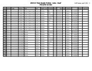
Chapter 5BC Ministry of ForestPamphlets TOCThe British Columbia Ministry of Forests has published a nice series of articleson common statistical queries. This is the table of contents 11 http://www.for.gov.bc.ca/research/biopamph/40

BIOMETRICSINFORMATIONIndex of Pamphlet Topics(for pamphlets #1 to #60) as of December, 2000Adjusted R-square18: Multiple regression: selecting the best subsetANCOVA: Analysis of Covariance13: ANCOVA: Analysis of Covariance31: ANCOVA: The linear models behind the F-testsANOVA: Analysis of Variance2: The importance of replication in analysis ofvariance3: ANOVA using SAS: specifying error terms4: ANOVA using SAS: How to pool error terms6: Using plot means for ANOVA9: Reading category variables with statisticssoftware14: ANOVA: Factorial designs with a separatecontrol16: ANOVA: Contrasts viewed as t-tests19: ANOVA: Approximate or Pseudo F-tests21: What are the degrees of freedom?22: ANOVA: Using a hand calculator to test a onewayANOVA23: ANOVA: Contrasts viewed as correlationcoefficients25: ANOVA: The within sums of squares as anaverage variance26: ANOVA: Equations for linear and quadraticcontrasts27: When the t-test and the F-test are equivalent28: Simple repression with replication: testing forlack of fit39: A repeated measures example40: Finding the expected mean squares and theproper error terms with SAS45: Calculating contrast F-tests when SAS will not48: ANOVA: Why a fixed effect is tested by itsinteraction with a random effect49: Power analysis and sample sizes for completelyrandomized designs with subsampling50: Power analysis and sample sizes for randomizedblock designs with subsampling51: Programs for power analysis/sample sizecalculations for CR and RB designs withsubsampling52: Post-hoc power analyses for ANOVA F-tests53: Balanced incomplete block (BIB) study designs54: Incomplete block designs: Connected designscan be analysed55: Displaying factor relationships in experiments56: The use of indicator variables in non-linearregression57: Interpreting main effects when a two-wayinteraction is present58: On the presentation of statistical results: asynthesis59: ANOVA: Coefficients for contrasts and meansof incomplete factorial designs60: MANOVA: Profile Analysis – an exampleusing SASASCII1: Producing ASCII files with SASBlocks17: What is the design?34: When are blocks pseudo-replicates?53: Balanced incomplete block (BIB) study designs54: Incomplete block designs: Connected designscan be analysedBonferroni13: ANCOVA: comparing adjusted meansBoxplots33: Box plotsChi-square Distribution15: Using SAS to obtain probability values for F-,t- and χ 2 statistics36: Contingency tables and log-linear models41Ministry of ForestsResearch Program

Cluster sampling43: Standard error formulas for cluster sampling(unequal cluster sizes)Completely Randomized Designs5: Understanding replication and pseudoreplication17: What is the design?48: ANOVA: Why a fixed effect is tested by itsinteraction with a random effect49: Power analysis and sample sizes for completelyrandomized designs with subsampling55: Displaying factor relationships in experiments57: Interpreting main effects when a two-wayinteraction is present59: ANOVA: Coefficients for contrasts and meansof incomplete factorial designsConfidence Intervals29: Simple Regression: Confidence intervals for apredicted X-value30: Interpretation of probability p-valuesConfidence Level11: Sample sizes: for one meanContingency Tables21: What are degrees of freedom?36: Contingency tables and log-linear models41: Power analysis and sample size determinationfor contingency table tests58: On the presentation of statistical results: asynthesisContrasts12: Determining polynomial contrast coefficients13: ANCOVA: comparing adjusted means14: ANOVA: Factorial designs with a separatecontrol16: ANOVA: Contrasts viewed as t-tests23: ANOVA: Contrasts viewed as correlationcoefficients26: ANOVA: Equations for linear and quadraticcontrasts45: Calculating contrast F-tests when SAS will not59: ANOVA: Coefficients for contrasts and meansof incomplete factorial designsControl14: ANOVA: Factorial designs with a separatecontrolCorrelation Coefficient23: ANOVA: Contrasts viewed as correlationcoefficientsCrossed Factors17: What is the design?48: ANOVA: Why a fixed effect is tested by itsinteraction with a random effect55: Displaying factor relationships in experiments57: Interpreting main effects when a two-wayinteraction is presentDegrees of Freedom19: ANOVA: Approximate or Pseudo F-tests21: What are degrees of freedom?Dunn-Bonferroni13: ANCOVA: comparing adjusted meansEDA (Exploratory Data Analysis)33: Box plotsError Bars38: Plotting error bars with SAS/GraphError Sums of Squares – see Residual sums ofsquares or Within sums of squaresError Terms3: ANOVA using SAS: specifying error terms4: ANOVA using SAS: How to pool error terms19: ANOVA: Approximate or Pseudo F-tests48: ANOVA: Why a fixed effect is tested by itsinteraction with a random effectExpected Mean Squares40: Finding the expected mean squares and theproper error terms with SAS422

Index of Pamphlet TopicsExperimental Design17: What is the design?34: When are blocks pseudo-replicates?44: What do we look for in a working plan?Experimental unit – see Treatment unitF-Distribution15: Using SAS to obtain probability values for F-,t-, and χ 2 statistics37: A general description of hypothesis testing andpower analysis52: Post-hoc power analyses for ANOVA F-testsF-Max Test25: ANOVA: The within sums of squares as anaverage varianceF-Test18: Multiple regression: selecting the best subject27: When the t-test and the F-test are equivalent28: Simple Regression with replication: testing forlack of fit31: ANCOVA: The linear models behind the F-tests45: Calculating contrast F-tests when SAS will not46: GLM: Comparing regression linesFactor Relationship Diagram55: Displaying factor relationships in experimentsFactorial Design14: ANOVA: Factorial designs with a separatecontrol17: What is the design?48: ANOVA: Why a fixed effect is tested by itsinteraction with a random effect53: Balanced incomplete block (BIB) study designs54: Incomplete block designs: Connected designscan be analysed55: Displaying factor relationships in experiments57: Interpreting main effects when a two-wayinteraction is present59: ANOVA: Coefficients for contrasts and meansof incomplete factorial designs60: MANOVA: Profile Analysis – an exampleusing SAS43Homogeneity of Variance25: ANOVA: The within sums of squares as anaverage varianceHypothesis Testing30: Interpretation of probability p-values37: A general description of hypothesis testing andpower analysis48: ANOVA: Why a fixed effect is tested by itsinteraction with a random effectIndicator (Dummy) Variables56: The use of indicator variables in non-linearregressionLack of Fit28: Simple regression with replication: testing forlack of fitLinear Combination16: ANOVA: Contrasts viewed as t-testsLinear Models28: Simple regression with replication for lack of fit31: ANCOVA: The linear models behind the F-tests46: GLM: Comparing regression linesLog-linear model36: Contingency tables and log-linear modelsLogistic Regression7: Logistic regression analysis: model statementsin PROC CATMODLSD (Least Significant Difference)13: ANCOVA: comparing adjusted means57: Interpreting main effects when a two-wayinteraction is presentMallow’s CP18: Multiple regression: selecting the best subset3

MANOVA39: A repeated measures example60: MANOVA: Profile Analysis – an exampleusing SASMeans6: Using plot means for ANOVA11: Sample sizes: for one mean43: Standard error formulas for cluster sampling(unequal cluster sizes)58: On the presentation of statistical results: asynthesis59: ANOVA: Coefficients for contrasts and meansof incomplete factorial designsMultiple Range Tests13: ANCOVA: comparing adjusted meansMultiple Regression8: Standard errors for predicted values frommultiple regression18: Multiple regression: selecting the best subset27: When the t-test and the F-test are equivalent56: The use of indicator variables in non-linearregressionNon-linear Regression39: A repeated measures example56: The use of indicator variables in non-linearregressionPolynomial Contrasts12: Determining polynomial contrast coefficients26: ANOVA: Equations for linear and quadraticcontrasts32: Analysing a split-plot in time with the properrepeated measures ANOVAPower37: A general description of hypothesis testing andpower analysis41: Power analysis and sample size determinationfor contingency table tests49: Power analysis and sample sizes for completelyrandomized designs with subsampling50: Power analysis and sample sizes for randomizedblock designs with subsampling51: Programs for power analysis/sample sizecalculations for CR and RB designs withsubsampling52: Post-hoc power analyses for ANOVA F-testsPredicted values8: Standard errors for predicted values frommultiple regression29: Simple Regression: Confidence intervals for apredicted X-valueProbability values15: Using SAS to obtain probability values for F-,t-, and χ 2 statistics30: Interpretation of probability p-valuesApproximate or Pseudo F-tests19: ANOVA: Approximate or Pseudo F-testsPseudo-Replication5: Understanding replication and pseudoreplication34: When are blocks pseudo-replicates?Questionnaire10: Results of biometrics questionnaireR-square18: Multiple regression: selecting the best subsetRandom Factors40: Finding the expected mean squares and theproper error terms with SAS48: ANOVA: Why a fixed effect is tested by itsinteraction with a random effectRandomized Block Designs5: Understanding replication and pseudoreplication17: What is the design?34: When are blocks of pseudo-replicates?50: Power analysis and sample sizes for randomizedblock designs with subsampling55: Displaying factor relationships in experiments444

Index of Pamphlet TopicsRegression21: What are degrees of freedom?27: When the t-test and the F-test are equivalent28: Simple regression with replication: testing forlack of fit29: Simple regression: Confidence intervals for apredicted X-value31: ANCOVA: The linear models behind the F-tests46: GLM Comparing regression lines56: The use of indicator variables in non-linearregression58: On the presentation of statistical results: asynthesisRepeated Measures32: Analysing a split-plot in time with the properrepeated measures ANOVA39: A repeated measures example58: On the presentation of statistical results: asynthesis60: MANOVA: Profile Analysis – an exampleusing SASReplication2: The importance of replication in analysis ofvariance5: Understanding replication and pseudoreplication17: What is the design?28: Simple regression with replication: testing forlack of fit48: ANOVA: Why a fixed effect is tested by itsinteraction with a random effectResidual Sums of Squares31: ANCOVA: The linear models behind the F-testsSample Size11: Sample sizes: for one mean41: Power analysis and sample size determinationfor contingency table tests49: Power analysis and sample sizes for completelyrandomized designs with subsampling50: Power analysis and sample sizes for randomizedblock designs with subsamplingSampling11: Sample sizes: for one mean43: Standard error formulas for cluster sampling(unequal cluster sizes)44: What do we look for in a working plan?Sampling Units17: What is the design?SAS Programs1: Producing ASCI files with SAS9: Reading category variables with statisticssoftware15: Using SAS to obtain probability values for F-,t-, and χ 2 statistics29: Simple Regression: Confidence intervals for apredicted X-value33: Box plots35: The computation of tree shadow lengths36: Contingency tables and log-linear models41: Power analysis and sample size determinationfor contingency table tests43: Standard error formulas for cluster sampling(unequal cluster sizes)47: SAS: Adding observations when class variables(e.g. species list) are missing51: Programs for power analysis/sample sizecalculations for CR and RB designs withsubsampling59: ANOVA: Coefficients for contrasts and meansof incomplete factorial designs60: MANOVA: Profile Analysis – an exampleusing SASSAS: CATMOD7: Logistic regression analysis: model statementsin PROC CATMOD36: Contingency tables and log-linear modelsSAS: Data Step20: Rearranging raw data files using SAS24: Reading WATFILE file into SAS47: SAS: Adding observations when class variables(e.g. species list) are missing455

SAS: GLM3: ANOVA using SAS: specifying error terms4: ANOVA using SAS: How to pool error terms6: Using plot means for ANOVA32: Analysing a split-plot in time with the properrepeated measures ANOVA40: Finding the expected mean squares and theproper error terms with SAS45: Calculating contrast F-tests when SAS will not46: GLM Comparing regression lines57: Interpreting main effects when a two-wayinteraction is present59: ANOVA: Coefficients for contrasts and meansof incomplete factorial designs60: MANOVA: Profile Analysis – an exampleusing SASSAS: Graph38: Plotting error bars with SAS/Graph42: Labelling curves in SAS/GRAPHSAS: MIXED59: ANOVA: Coefficients for contrasts and meansof incomplete factorial designsSAS: NLIN39: A repeated measures example56: The use of indicator variables in non-linearregressionSAS: REG8: Standard errors for predicted values frommultiple regression18: Multiple regression: selecting the best subsetShadow Lengths35: The computation of Tree Shadow LengthsSplit-Plot Design6: Using plot means for ANOVA17: What is the design?32: Analysing a split-plot in time with the properrepeated measures ANOVA34: When are blocks pseudo-replicates?55: Displaying factor relationships in experimentsStandard Errors8: Standard errors for predicted values frommultiple regression11: Sample sizes: for one mean43: Standard error formulas for cluster sampling(unequal cluster sizes)58: On the presentation of statistical results: asynthesis59: ANOVA: Coefficients for contrasts and meansof incomplete factorial designsSYSTAT9: Reading category variables with statisticssoftwaret-distribution15: Using SAS to obtain probability values for F-,t-, and χ 2 statisticst-test16: ANOVA: Contrasts viewed as t-tests27: When the t-test and the F-test are equivalentTreatment Unit2: The importance of replication in analysis ofvariance5: Understanding replication and pseudoreplication17: What is the design?34: When are blocks pseudo-replicates?55: Displaying factor relationships in experimentsType I & II errors30: Interpretation of probability p-values37: A general description of hypothesis testing andpower analysisWATFILE24: Reading WATFILE file into SASWithin Sums of Squares25: ANOVA: The within sums of squares as anaverage variance28: Simple regression with replication: testing forlack of fit646

Chapter 6How do I interpret a p-valuep-values are prone to mis-interpretation as they measure the plausibility of thedata assuming the null hypothsis is true, not the probability that the hypothesisis true. There is also the confusion between selecting the appropriate p-valuefor one- and two-sided tests.This is a copy of the BC Ministry of Forest pamphlet on interpreting p-values.It is available at: interpreting the p-value 11 http://www.for.gov.bc.ca/research/biopamph/47

BIOMETRICSINFORMATION(You’re 95% likely to need this information)PAMPHLET NO. # 30 DATE: March 5, 1991SUBJECT:Interpretation of probability p-valuesMost statistical computer programs, including SAS, calculate and report probability or p-valuesin their output. These values can then be used to make conclusions about associated hypotheses.This pamphlet will discuss the use and interpretation of these p-values.For example, a fertilizer supplier claims that a new type of fertilizer can increase the averagegrowth rate of a certain type of tree. To test this claim, two random samples of these trees areselected and treated with the "new" fertilizer and the standard fertilizer respectively. The objectiveis to determine if the trees treated with the new fertilizer have a higher growth rate than the treestreated with the standard fertilizer.In hypothesis testing, two contradictory hypotheses are under consideration. The nullhypothesis H o states an equality between population parameters, for example, trees treated withthe new fertilizer have the same growth rate as trees treated with the standard fertilizer. Thealternate hypothesis H a states a difference between parameters and is usually what the experimenterhopes to verify, for example, trees treated with the new fertilizer have a better growth rate thantrees treated with the standard fertilizer. The null hypothesis will be rejected if the sampleevidence is more consistent with the alternative hypothesis.When drawing a conclusion in hypothesis testing, one is faced with the possibility of makingtwo types of errors. A Type I error consists of rejecting H o when it is true and a Type II errorinvolves not rejecting H o when it is false. The probability of making a type I error is traditionallydenoted by α , and the probability of making a type II error by β . Often the value α isspecified to indicate the amount of Type I error one is willing to tolerate. This α value isreferred to as the significance level of the test. Typically acceptable α-levels are 0.05 and 0.01.If, for example, one concludes that the growth rate of trees treated with the new fertilizer issignificantly different from those treated with the standard fertilizer at α = 0.05, then there is a 5%chance that the conclusion is wrong.While reporting the result of an hypothesis test, stating that H o is rejected at some α level isnot sufficient as it does not provide information on the weight of evidence against it. Also, itdictates the α-level that others must use. A more appropriate approach is to report the p-value:the smallest level at which the data is significant. H o is rejected at the α-level only if the p-valueis less than α . Suppose the p-value of the above fertilizer test is 0.02, that is, if one were toreject H o based on the data, then there is a 2% chance that the decision is incorrect. At α = 0.05,the experimenter would reject H o as the Type I error (2%) in the data is within the allowedamount of 5% specified. Conversely, at α 48 = 0.01, the experimenter would retain H o as theMinistry of ForestsResearch Program

2Type I error in the data exceeds what he/she is willing to tolerate. That is, the test is significant at5% level but not significant at 1%. In fact, p-value measures the amount of statistical evidenceagainst the null hypothesis in favor of the alternative hypothesis: the smaller the p-value thestronger the evidence against the null hypothesis. When drawing a conclusion, the weight ofevidence indicated by the computed p-value should be reported. This weight of evidence may beindicated in words according to the following table:Weight of evidence againstp-value = pthe null hypothesissssssssssssssssssssssssssssssssssssssssssssssssssssssssssssssssssssssp ≤ 0.01very strong0.01 < p ≤ 0.05 strong0.05 < p ≤ 0.10 moderate0.10 < p little or noExample 1: Suppose two different fertilizers (1 and 2) are available and one is interested intesting if there is a difference in performance between them. Two samples of trees are randomlyselected and each is treated with one of the two fertilizers and the growth rate (Y) is measured.This test can be carried out using PROC ANOVA or PROC GLM with class variable A indicatingthe type of fertilizer (1 or 2) applied. The required model statement is MODEL Y = A . The SASoutput consists of an ANOVA table with the p-value of the test. If a p-value of 0.35 was obtained,the conclusion would be: "There is no evidence (p = 0.35) that the two fertilizers performdifferently."Example 2: Suppose further that an experiment had treatments with the following levels: acontrol (no fertilizer), a standard fertilizer, and a new fertilizer applied at two different amounts.The experimenter might have the following questions:1. Is the control different from the other treatments?2. Is the standard fertilizer different from the new fertilizer?3. Are the two different levels for the new fertilizer producing different responses?These questions could be answered with the following contrasts:Contrasts Coefficientsfor QuestionTreatmentssssssssssssssss1 2 3ssssssssssssssssssssssssssssssssssssssControl -3 0 0Standard 1 -2 0New: level 1 1 1 -1New: level 2 1 1 149

3 Pamphlet #30rrrrrrrrrrrrrrrrrrrrrPROC GLM with the appropriate contrast statements could be used to test the contrasts. Thep-values for the contrasts are computed and reported as part of the SAS output. If the p-value forquestion 1 was 0.015, then the conclusion would be: "There is strong evidence (p = 0.015) that thecontrol is different from the other treatments."Example 3: Suppose it is believed that the growth rate (Y) is linearly dependent on theamount of fertilizer applied (X). To test this claim, fit a regression line Y = β 0 + β 1 X and testthe hypotheses H o : β 1 = 0 vs H a : β 1 ≠ 0 . This can be accomplished using PROG REGwith the model statement MODEL Y = X . SAS will compute the estimated values of β 0 and β 1 ,perform an F-test and report the p-value under the column "PROB > F". If a p-value of 0.023 wasobtained, the conclusion could be stated as follows: "There is strong evidence (p = 0.023) that theamount of fertilizer applied affects the growth rate."Example 4: Suppose one is interested in testing if there is a relationship between tree speciesand success in seed germination. Count data of the number of germinated seeds from each treespecies is available for analysis by a contingency table. SAS has 2 procedures to do this:PROC FREQ can be used for two dimensional tables only while PROC CATMOD is suitable forany dimensional table. If PROC FREQ was used, the statementTABLE SPECIES*SEED/CELLCHI2 CHISQwould produce a two-way frequency table of species by seed with the χ 2 statistics due to eachcell printed. The total χ 2 statistic and the corresponding p-value would also be reported. If ap-value of 0.084 was obtained, then the conclusion would be: "There is moderate evidence(p = 0.084) that success in seed germination is different for the different tree species."In short, p-values convey information about the strength of evidence against the nullhypothesis and allow an individual to draw a conclusion at any specific level α. Nevertheless, αshould not be the only criteria for decision making. When the null hypothesis is not rejected, β ,the size of the Type II error should also be reported. A false H o could have been missed if β islarge in the experiment due to a small sample size or large sampling variability. This topic ofPower Analysis will be explored in future pamphlets.References:Devore, J.L., 1987. Probability and Statistics for Engineering and the Science. 2nd ed. Brooks/ColePublishing Company.Stafford, S.G., A Statistics Primer for Foresters, Journal of Forestry, March 1985, p 148-157.50CONTACT: Vera Sit or Wendy Bergerud356-0435 387-5676

4ssssssssssssssssssssssssssssssssssssssssssssssssssssssssNEW PROBLEMssssssssssssssssssssssssssssssssssssssssssssssssssssssssList the null hypotheses for the three questions posed in example 2.ssssssssssssssssssssssssssssssssssssssssssssssssPROBLEM FROM BI# 29ssssssssssssssssssssssssssssssssssssssssssssssssssssIn order to compute the 90% confidence interval, the value in the tinv statement should bechanged from 0.975 to 0.95.SAS Output for Problem:Point Estimate and 90% Confidence Interval of X on a Given YModel :Y=ahat + bhat * XAHAT BHAT64.2468 -1.01299------------------------ GROUP=1 --------------------No. ofY-values Mean of Estimated Lower Upperused Given Y X Limit Limit1 40 23.9359 37.8890 11.6352ssssssssssssssssssssssssssssssssssssssssssssssssssssssssssssssssssssssssssssssssssssssssssssssssssssssssssssssssssssssssssssssssssssssss51

Chapter 7The results are significant(p < .05) - NOT!Is it necessary to have a p-value in every publication? The article below arguesthat it is not and also points out some of the dangers of an uncritical use ofhypothesis testing.Cherry, S. (1998)Statistical tests in publication of the Wildlife SocietyWildlife Society Bulletin, 26, 947-954.Not available on the web.52

Chapter 8The Insignificance ofStatistical SignificanceTestingJohnson, D. H. (1999)The Insignificance of Statistical Significance TestingJournal of Wildlife Management, 63, 763-772.Despite their wide use in scientific journals such as The Journal of WildlifeManagement, statistical hypothesis tests add very little value to the products ofresearch. Indeed, they frequently confuse the interpretation of data. This paperdescribes how statistical hypothesis tests are often viewed, and then contraststhat interpretation with the correct one. He discuss the arbitrariness of p-values,conclusions that the null hypothesis is true, power analysis, and distinctionsbetween statistical and biological significance. Statistical hypothesis testing,in which the null hypothesis about the properties of a population is almostalways known a priori to be false, is contrasted with scientific hypothesis testing,which examines a credible null hypothesis about phenomena in nature. Moremeaningful alternatives are briefly outlined, including estimation and confidenceintervals for determining the importance of factors, decision theory for guidingactions in the face of uncertainty, and Bayesian approaches to hypothesis testingand other statistical practices.Also available on the web at 11 http://www.npwrc.usgs.gov/resource/1999/statsig/statsig.htm60

Statistical Signigicance TestingThe Insignificance of StatisticalSignificance TestingBy Douglas H. Johnson 1Abstract: Despite their wide use in scientific journals such as The Journal of Wildlife Management, statisticalhypothesis tests add very little value to the products of research. Indeed, they frequently confuse theinterpretation of data. This paper describes how statistical hypothesis tests are often viewed, and then contraststhat interpretation with the correct one. I discuss the arbitrariness of P-values, conclusions that the nullhypothesis is true, power analysis, and distinctions between statistical and biological significance. Statisticalhypothesis testing, in which the null hypothesis about the properties of a population is almost always known apriori to be false, is contrasted with scientific hypothesis testing, which examines a credible null hypothesisabout phenomena in nature. More meaningful alternatives are briefly outlined, including estimation andconfidence intervals for determining the importance of factors, decision theory for guiding actions in the faceof uncertainty, and Bayesian approaches to hypothesis testing and other statistical practices.Key words: Bayesian approaches, confidence interval, null hypothesis, P-value, power analysis, scientifichypothesis test, statistical hypothesis test.This resource is based on the following source (Northern Prairie Publication 1057):Johnson, Douglas H. 1999. The Insignificance of Statistical SignificanceTesting. Journal of Wildlife Management 63(3):763-772.This resource should be cited as:Johnson, Douglas H. 1999. The Insignificance of Statistical SignificanceTesting. Journal of Wildlife Management 63(3):763-772. Jamestown,ND: Northern Prairie Wildlife Research Center Home Page.http://www.npwrc.usgs.gov/resource/1999/statsig/statsig.htm(Version 16SEP99).Editor's Note: Doug Johnson received The Wildlife Society Award for Outstanding Publication in Wildlife61http://www.npwrc.usgs.gov/resource/1999/statsig/statsig.htm (1 of 3) [12/6/2002 3:10:51 PM]

Statistical Signigicance TestingEcology and Management, in the Article Category for this paper. The award was conferred at the Society'sannual meeting, 13 September 2000, in Nashville, Tennessee.President of The Wildlife Society, Nova Silvy (right), presents Doug Johnson (left)with the Outstanding Publication Award.Table of ContentsIntroductionWhat is Statistical Hypothesis Testing?❍ What are More Extreme Data?❍ Are Null Hypotheses Really True?❍ P is Arbitrary❍ Proving the Null Hypothesis❍ Power Analysis❍ Biological Versus Statistical Significance❍ Other Comments on Hypothesis TestsWhy Are Hypothesis Tests UsedReplicationWhat are the Alternatives62http://www.npwrc.usgs.gov/resource/1999/statsig/statsig.htm (2 of 3) [12/6/2002 3:10:51 PM]

Statistical Signigicance Testing❍ Estimates and Confidence Intervals❍ Decision Theory❍ Model Selection❍ Bayesian ApproachesConclusionsAcknowledgementsLiterature Cited1 U.S. Geological Survey, Biological Resources Division, Northern Prairie Wildlife Research Center,Jamestown, ND 58401, USAE-mail: douglas_h_johnson@usgs.govDownloading Instructions -- Instructions on downloading and extracting files from this site.statsig.zip (40484 bytes) -- The Insignificance of Statistical Significance TestingInstallation: Extract all files and open statsig.htm in a web browser.Northern Prairie Wildlife Research CenterHome | Site Map | Biological Resources | Help & Feedback63http://www.npwrc.usgs.gov/resource/1999/statsig/statsig.htm (3 of 3) [12/6/2002 3:10:51 PM]

Statistical Signigicance TestingThe Insignificance of StatisticalSignificance TestingIntroductionStatistical testing of hypotheses in the wildlife field has increased dramatically in recent years. Evenmore recent is an emphasis on power analysis associated with hypothesis testing (The Wildlife Society1995). While this trend was occurring, statistical hypothesis testing was being deemphasized in someother disciplines. As an example, the American Psychological Association seriously debated a ban onpresenting results of such tests in the Association's scientific journals. That proposal was rejected, notbecause it lacked merit, but due to its appearance of censorship (Meehl 1997).The issue was highlighted at the 1998 annual conference of The Wildlife Society, in Buffalo, New York,where the Biometrics Working Group sponsored a half-day symposium on Evaluating the Role ofHypothesis Testing–Power Analysis in Wildlife Science. Speakers at that session who addressedstatistical hypothesis testing were virtually unanimous in their opinion that the tool was overused,misused, and often inappropriate.My objectives are to briefly describe statistical hypothesis testing, discuss common but incorrectinterpretations of resulting P-values, mention some shortcomings of hypothesis testing, indicate whyhypothesis testing is conducted, and outline some alternatives.Return to ContentsNext Section -- What is Statistical Hypothesis Testing?Northern Prairie Wildlife Research CenterHome | Site Map | Biological Resources | Help & Feedback64http://www.npwrc.usgs.gov/resource/1999/statsig/intro.htm [12/6/2002 3:10:56 PM]

Statistical Significance TestingThe Insignificance of StatisticalSignificance TestingWhat is Statistical Hypothesis Testing?Four basic steps constitute statistical hypothesis testing. First, one develops a null hypothesis about somephenomenon or parameter. This null hypothesis is generally the opposite of the research hypothesis,which is what the investigator truly believes and wants to demonstrate. Research hypotheses may begenerated either inductively, from a study of observations already made, or deductively, deriving fromtheory. Next, data are collected that bear on the issue, typically by an experiment or by sampling. (Nullhypotheses often are developed after the data are in hand and have been rummaged through, but that'sanother topic.) A statistical test of the null hypothesis then is conducted, which generates a P-value.Finally, the question of what that value means relative to the null hypothesis is considered. Severalinterpretations of P often are made.Sometimes P is viewed as the probability that the results obtained were due to chance. Small values aretaken to indicate that the results were not just a happenstance. A large value of P, say for a test that µ = 0,would suggest that the mean actually recorded was due to chance, and µ could be assumed to be zero(Schmidt and Hunter 1997).Other times, 1-P is considered the reliability of the result, that is, the probability of getting the sameresult if the experiment were repeated. Significant differences are often termed "reliable" under thisinterpretation.Alternatively, P can be treated as the probability that the null hypothesis is true. This interpretation is themost direct one, as it addresses head-on the question that interests the investigator.These 3 interpretations are what Carver (1978) termed fantasies about statistical significance. None ofthem is true, although they are treated as if they were true in some statistical textbooks and applicationspapers. Small values of P are taken to represent strong evidence that the null hypothesis is false, butworkers demonstrated long ago (see references in Berger and Sellke 1987) that such is not the case. Infact, Berger and Sellke (1987) gave an example for which a P-value of 0.05 was attained with a sample65http://www.npwrc.usgs.gov/resource/1999/statsig/stathyp.htm (1 of 7) [12/6/2002 3:10:59 PM]

Statistical Significance Testingof n = 50, but the probability that the null hypothesis was true was 0.52. Further, the disparity between Pand Pr[H 0 | data], the probability of the null hypothesis given the observed data, increases as samplesbecome larger.In reality, P is the Pr[observed or more extreme data | H 0 ], the probability of the observed data or datamore extreme, given that the null hypothesis is true, the assumed model is correct, and the sampling wasdone randomly. Let us consider the first two assumptions.What are More Extreme Data?Suppose you have a sample consisting of 10 males and three females. For a null hypothesis of a balancedsex ratio, what samples would be more extreme? The answer to that question depends on the samplingplan used to collect the data (i.e., what stopping rule was used). The most obvious answer is based on theassumption that a total of 13 individuals were sampled. In that case, outcomes more extreme than 10males and 3 females would be 11 males and 2 females, 12 males and 1 female, and 13 males and nofemales.However, the investigator might have decided to stop sampling as soon as he encountered 10 males.Were that the situation, the possible outcomes more extreme against the null hypothesis would be 10males and 2 females, 10 males and 1 female, and 10 males and no females. Conversely, the investigatormight have collected data until 3 females were encountered. The number of more extreme outcomes thenare infinite: they include 11 males and 3 females, 12 males and 3 females, 13 males and 3 females, etc.Alternatively, the investigator might have collected data until the difference between the numbers ofmales and females was 7, or until the difference was significant at some level. Each set of more extremeoutcomes has its own probability, which, along with the probability of the result actually obtained,constitutes P.The point is that determining which outcomes of an experiment or survey are more extreme than theobserved one, so a P-value can be calculated, requires knowledge of the intentions of the investigator(Berger and Berry 1988). Hence, P, the outcome of a statistical hypothesis test, depends on results thatwere not obtained, that is, something that did not happen, and what the intentions of the investigatorwere.Are Null Hypotheses Really True?P is calculated under the assumption that the null hypothesis is true. Most null hypotheses tested,however, state that some parameter equals zero, or that some set of parameters are all equal. Thesehypotheses, called point null hypotheses, are almost invariably known to be false before any data arecollected (Berkson 1938, Savage 1957, Johnson 1995). If such hypotheses are not rejected, it is usuallybecause the sample size is too small (Nunnally 1960).66http://www.npwrc.usgs.gov/resource/1999/statsig/stathyp.htm (2 of 7) [12/6/2002 3:10:59 PM]

Statistical Significance TestingTo see if the null hypotheses being tested in The Journal of Wildlife Management can validly beconsidered to be true, I arbitrarily selected two issues: an issue from the 1996 volume, the other from1998. I scanned the results section of each paper, looking for P-values. For each P-value I found, Ilooked back to see what hypothesis was being tested. I made a very biased selection of some conclusionsreached by rejecting null hypotheses; these include: (1) the occurrence of sheep remains in coyote (Canislatrans) scats differed among seasons (P = 0.03, n = 467), (2) duckling body mass differed among years(P < 0.0001), and (3) the density of large trees was greater in unlogged forest stands than in loggedstands (P = 0.02). (The last is my personal favorite.) Certainly we knew before any data were collectedthat the null hypotheses being tested were false. Sheep remains certainly must have varied amongseasons, if only between 61.1% in 1 season and 61.2% in another. The only question was whether or notthe sample size was sufficient to detect the difference. Likewise, we know before data are collected thatthere are real differences in the other examples, which are what Abelson (1997) referred to as"gratuitous" significance testing—testing what is already known.Three comments in favor of the point null hypothesis, such as µ = µ 0 . First, while such hypotheses arevirtually always false for sampling studies, they may be reasonable for experimental studies in whichsubjects are randomly assigned to treatment groups (Mulaik et al. 1997). Second, testing a point nullhypothesis in fact does provide a reasonable approximation to a more appropriate question: is µ nearlyequal to µ 0 (Berger and Delampady 1987, Berger and Sellke 1987), if the sample size is modest(Rindskopf 1997). Large sample sizes will result in small P-values even if µ is nearly equal to µ 0 . Third,testing the point null hypothesis is mathematically much easier than testing composite null hypotheses,which involve noncentrality parameters (Steiger and Fouladi 1997).The bottom line on P-values is that they relate to data that were not observed under a model that isknown to be false. How meaningful can they be? But they are objective, at least; or are they?P is ArbitraryIf the null hypothesis truly is false (as most of those tested really are), then P can be made as small as onewishes, by getting a large enough sample. P is a function of (1) the difference between reality and thenull hypothesis and (2) the sample size. Suppose, for example, that you are testing to see if the mean of apopulation (µ) is, say, 100. The null hypothesis then is H 0 : µ = 100, versus the alternative hypothesis ofH 1 : µ 100. One might use Student's t-test, which iswhere is the mean of the sample, S is the standard deviation of the sample, and n is the sample size.Clearly, t can be made arbitrarily large (and the P-value associated with it arbitrarily small) by makingeither ( – 100) or large enough. As the sample size increases, ( – 100) and S will67http://www.npwrc.usgs.gov/resource/1999/statsig/stathyp.htm (3 of 7) [12/6/2002 3:10:59 PM]

Statistical Significance Testingapproximately stabilize at the true parameter values. Hence, a large value of n translates into a largevalue of t. This strong dependence of P on the sample size led Good (1982) to suggest that P-values bestandardized to a sample size of 100, by replacing P by P(or 0.5, if that is smaller).Even more arbitrary in a sense than P is the use of a standard cutoff value, usually denoted . P-valuesless than or equal to are deemed significant; those greater than are nonsignificant. Use of wasadvocated by Jerzy Neyman and Egon Pearson, whereas R. A. Fisher recommended presentation ofobserved P-values instead (Huberty 1993). Use of a fixed level, say = 0.05, promotes the seeminglynonsensical distinction between a significant finding if P = 0.049, and a nonsignificant finding if P =0.051. Such minor differences are illusory anyway, as they derive from tests whose assumptions often areonly approximately met (Preece 1990). Fisher objected to the Neyman-Pearson procedure because of itsmechanical, automated nature (Mulaik et al. 1997).Proving the Null HypothesisDiscourses on hypothesis testing emphasize that null hypotheses cannot be proved; they can only bedisproved (rejected). Failing to reject a null hypothesis does not mean that it is true. Especially withsmall samples, one must be careful not to accept the null hypothesis. Consider a test of the nullhypothesis that a mean µ equals µ 0 . The situations illustrated in Figure 1 both reflect a failure to rejectthat hypothesis. Figure 1A suggests the null hypothesis may well be false, but the sample was too smallto indicate significance; there is a lack of power. Conversely, Figure 1B shows that the data truly wereconsistent with the null hypothesis. The two situations should lead to different conclusions about µ, butthe P-values associated with the tests are identical.Taking another look at the two issues of The Journal of Wildlife Management, I noted a number ofarticles that indicated a null hypothesis was proven. Among these were (1) no difference in slope aspectof random snags (P = 0.112, n = 57), (2) no difference in viable seeds (F 2,6 = 3.18, P = 0.11), (3) lambkill was not correlated to trapper hours (r 12 = 0.50, P = 0.095), (4) no effect due to month (P = 0.07, n =15), and (5) no significant differences in survival distributions (P-values > 0.014!, n variable). I selectedthe examples to illustrate null hypotheses claimed to be true, despite small sample sizes and P-values thatwere small but (usually) >0.05. All examples, I believe, reflect the lack of power (Fig. 1A) whileclaiming a lack of effect (Fig. 1B).68http://www.npwrc.usgs.gov/resource/1999/statsig/stathyp.htm (4 of 7) [12/6/2002 3:10:59 PM]

Statistical Significance TestingFig 1. Results of a test that failed to reject the null hypothesis that a mean equals 0.Shaded areas indicate regions for which hypothesis would be rejected. (A) suggests thenull hypothesis may well be false, but the sample was too small to indicate significance;there is a lack of power. (B) suggests the data truly were consistent with the nullhypothesisPower AnalysisPower analysis is an adjunct to hypothesis testing that has become increasingly popular (Peterman 1990,Thomas and Krebs 1997). The procedure can be used to estimate the sample size needed to have aspecified probability (power = 1 - ) of declaring as significant (at the level) a particular difference oreffect (effect size). As such, the process can usefully be used to design a survey or experiment (Gerard etal. 1998). Its use is sometimes recommended to ascertain the power of the test after a study has beenconducted and nonsignificant results obtained (The Wildlife Society 1995). The notion is to guardagainst wrongly declaring the null hypothesis to be true. Such retrospective power analysis can bemisleading, however. Steidl et al. (1997:274) noted that power estimated with the data used to test thenull hypothesis and the observed effect size is meaningless, as a high P-value will invariably result inlow estimated power. Retrospective power estimates may be meaningful if they are computed with effectsizes different from the observed effect size. Power analysis programs, however, assume the input valuesfor effect and variance are known, rather than estimated, so they give misleadingly high estimates ofpower (Steidl et al. 1997, Gerard et al. 1998). In addition, although statistical hypothesis testing invokeswhat I believe to be 1 rather arbitrary parameter ( or P), power analysis requires three of them ( , ,effect size). For further comments see Shaver (1993:309), who termed power analysis "a vacuousintellectual game," and who noted that the tendency to use criteria, such as Cohen's (1988) standards forsmall, medium, and large effect sizes, is as mindless as the practice of using the = 0.05 criterion instatistical significance testing. Questions about the likely size of true effects can be better addressed withconfidence intervals than with retrospective power analyses (e.g., Steidl et al. 1997, Steiger and Fouladi1997).69http://www.npwrc.usgs.gov/resource/1999/statsig/stathyp.htm (5 of 7) [12/6/2002 3:10:59 PM]

Statistical Significance TestingBiological Versus Statistical SignificanceMany authors make note of the distinction between statistical significance and subject-matter (in ourcase, biological) significance. Unimportant differences or effects that do not attain significance are okay,and important differences that do show up significant are excellent, for they facilitate publication (Table1). Unimportant differences that turn out significant are annoying, and important differences that failstatistical detection are truly depressing. Recalling our earlier comments about the effect of sample sizeon P-values, the two outcomes that please the researcher suggest the sample size was about right (Table2). The annoying unimportant differences that were significant indicate that too large a sample wasobtained. Further, if an important difference was not significant, the investigator concludes that thesample was insufficient and calls for further research. This schizophrenic nature of the interpretation ofsignificance greatly reduces its value.Table 1. Reaction of investigator to results of astatistical significance test (after Nester 1996).Statistical significancePracticalimportance ofobservedNot significant SignificantdifferenceNot important Happy AnnoyedImportant Very sad ElatedTable 2. Interpretation of sample size as relatedto results of a statistical significance test.Statistical significancePracticalimportance ofobservedNot significant SignificantdifferenceNot important n okay n too bigImportant n too small n okayOther Comments on Hypothesis TestsStatistical hypothesis testing has received an enormous amount of criticism, and for a rather long time. In1963, Clark (1963:466) noted that it was "no longer a sound or fruitful basis for statistical investigation."Bakan (1966:436) called it "essential mindlessness in the conduct of research." The famed quality guruW. Edwards Deming (1975) commented that the reason students have problems understandinghypothesis tests is that they may be trying to think. Carver (1978) recommended that statisticalsignificance testing should be eliminated; it is not only useless, it is also harmful because it is interpretedto mean something else. Guttman (1985) recognized that "In practice, of course, tests of significance arenot taken seriously." Loftus (1991) found it difficult to imagine a less insightful way to translate data intoconclusions. Cohen (1994:997) noted that statistical testing of the null hypothesis "does not tell us whatwe want to know, and we so much want to know what we want to know that, out of desperation, wenevertheless believe that it does!" Barnard (1998:47) argued that "... simple P-values are not now used bythe best statisticians." These examples are but a fraction of the comments made by statisticians and usersof statistics about the role of statistical hypothesis testing. While many of the arguments againstsignificance tests stem from their misuse, rather than their intrinsic values (Mulaik et al. 1997), I believe70http://www.npwrc.usgs.gov/resource/1999/statsig/stathyp.htm (6 of 7) [12/6/2002 3:10:59 PM]

Statistical Significance Testingthat 1 of their intrinsic problems is that they do encourage misuse.Previous Section -- IntroductionReturn to ContentsNext Section -- Why are Hypothesis Tests UsedNorthern Prairie Wildlife Research CenterHome | Site Map | Biological Resources | Help & Feedback71http://www.npwrc.usgs.gov/resource/1999/statsig/stathyp.htm (7 of 7) [12/6/2002 3:10:59 PM]

Statistical Significance TestingThe Insignificance of StatisticalSignificance TestingWhy are Hypothesis Tests Used?With all the deficiencies of statistical hypothesis tests, it is reasonable to wonder why they remain sowidely used. Nester (1996) suggested several reasons: (1) they appear to be objective and exact; (2) theyare readily available and easily invoked in many commercial statistics packages; (3) everyone else seemsto use them; (4) students, statisticians, and scientists are taught to use them; and (5) some journal editorsand thesis supervisors demand them. Carver (1978) recognized that statistical significance is generallyinterpreted as having some relationship to replication, which is the cornerstone of science. Morecynically, Carver (1978) suggested that complicated mathematical procedures lend an air of scientificobjectivity to conclusions. Shaver (1993) noted that social scientists equate being quantitative with beingscientific. D. V. Lindley (quoted in Matthews 1997) observed that "People like conventional hypothesistests because it's so easy to get significant results from them."I attribute the heavy use of statistical hypothesis testing, not just in the wildlife field but in other "soft"sciences such as psychology, sociology, and education, to "physics envy." Physicists and otherresearchers in the "hard" sciences are widely respected for their ability to learn things about the realworld (and universe) that are solid and incontrovertible, and also yield results that translate into productsthat we see daily. Psychologists, for one group, have difficulty developing tests that are able todistinguish two competing theories.In the hard sciences, hypotheses are tested; that process is an integral component of thehypothetico–deductive scientific method. Under that method, a theory is postulated, which generatesseveral predictions. These predictions are treated as scientific hypotheses, and an experiment isconducted to try to falsify each hypothesis. If the results of the experiment refute the hypothesis, thatoutcome implies that the theory is incorrect and should be modified or scrapped. If the results do notrefute the hypothesis, the theory stands and may gain support, depending on how critical the experimentwas.72http://www.npwrc.usgs.gov/resource/1999/statsig/whyused.htm (1 of 3) [12/6/2002 3:11:01 PM]

Statistical Significance TestingIn contrast, the hypotheses usually tested by wildlife ecologists do not devolve from general theoriesabout how the real world operates. More typically they are statistical hypotheses (i.e., statements aboutproperties of populations; Simberloff 1990). Unlike scientific hypotheses, the truth of which is truly inquestion, most statistical hypotheses are known a priori to be false. The confusion of the 2 types ofhypotheses has been attributed to the pervasive influence of R. A. Fisher, who did not distinguish them(Schmidt and Hunter 1997).Scientific hypothesis testing dates back at least to the 17th century: in 1620, Francis Bacon discussed therole of proposing alternative explanations and conducting explicit tests to distinguish between them asthe most direct route to scientific understanding (Quinn and Dunham 1983). This concept is related toPopperian inference, which seeks to develop and test hypotheses that can clearly be falsified (Popper1959), because a falsified hypothesis provides greater advance in understanding than does a hypothesisthat is supported. Also similar is Platt's (1964) notion of strong inference, which emphasizes developingalternative hypotheses that lead to different predictions. In such a case, results inconsistent withpredictions from a hypothesis cast doubt of its validity.Examples of scientific hypotheses, which were considered credible, include Copernicus' notion H A : theEarth revolves around the sun, versus the conventional wisdom of the time H 0 : the sun revolves aroundthe Earth. Another example is Fermat's last theorem, which states that for integers n, X, Y, and Z, X n + Y n= Z n implies n < 2. Alternatively, a physicist may make specific predictions about a parameter based on atheory, and the theory is provisionally accepted only if the outcomes are within measurement error of thepredicted value, and no other theories make predictions that also fall within that range (Mulaik et al.1997). Contrast these hypotheses, which involve phenomena in nature, with the statistical hypothesespresented in The Journal of Wildlife Management, which were mentioned above, and which involveproperties of populations.Rejection of a statistical hypothesis would constitute a piece of evidence to be considered in decidingwhether or not to reject a scientific hypothesis (Simberloff 1990). For example, a scientific hypothesismight state that clutch sizes of birds increase with the age of the bird, up to some plateau. That ideawould generate a hypothesis that could be tested statistically within a particular population of birds. Asingle such test, regardless of its P-value, would little affect the credibility of the scientific hypothesis,which is far more general. A related distinction is that scientific hypotheses are global, applying to all ofnature, while statistical hypotheses are local, applying to particular systems (Simberloff 1990).Why do we wildlife ecologists rarely test scientific hypotheses? My view is that we are dealing withsystems more complex than those faced by physicists. A saying in ecology is that everything isconnected to everything else. (In psychology, "everything correlates with everything," giving rise to whatDavid Lykken called the "crud factor" for such ambient correlation noise [Meehl 1997]). This sayingimplies that all variables in an ecological system are intercorrelated, and that any null hypothesispostulating no effect of a variable on another will in fact be false; a statistical test of that hypothesis willbe rejected, as long as the sample is sufficiently large. This line of reasoning does not denigrate the valueof experimentation in real systems; ecologists should seek situations in which variables thought to be73http://www.npwrc.usgs.gov/resource/1999/statsig/whyused.htm (2 of 3) [12/6/2002 3:11:01 PM]

Statistical Significance Testinginfluential can be manipulated and the results carefully monitored (Underwood 1997). Too often,however, experimentation in natural systems is very difficult if not impossible.Previous Section -- What is Statistical Hypothesis Testing?Return to ContentsNext Section -- ReplicationNorthern Prairie Wildlife Research CenterHome | Site Map | Biological Resources | Help & Feedback74http://www.npwrc.usgs.gov/resource/1999/statsig/whyused.htm (3 of 3) [12/6/2002 3:11:01 PM]

Statistical Significance TestingThe Insignificance of StatisticalSignificance TestingReplicationReplication is a cornerstone of science. If results from a study cannot be reproduced, they have nocredibility. Scale is important here. Conducting the same study at the same time but at several differentsites and getting comparable results is reassuring, but not nearly so convincing as having differentinvestigators achieve similar results using different methods in different areas at different times. R. A.Fisher's idea of solid knowledge was not a single extremely significant result, but rather the ability ofrepeatedly getting results significant at 5% (Tukey 1969). Shaver (1993:304) observed that "The questionof interest is whether an effect size of a magnitude judged to be important has been consistently obtainedacross valid replications. Whether any or all of the results are statistically significant is irrelevant."Replicated results automatically make statistical significance testing unnecessary (Bauernfeind 1968).Individual studies rarely contain sufficient information to support a final conclusion about the truth orvalue of a hypothesis (Schmidt and Hunter 1997). Studies differ in design, measurement devices,samples included, weather conditions, and many other ways. This variability among studies is morepervasive in ecological situations than in, for example, the physical sciences (Ellison 1996). To havegenerality, results should be consistent under a wide variety of circumstances. Meta-analysis providessome tools for combining information from repeated studies (e.g., Hedges and Olkin 1985) and canreduce dependence on significance testing by examining replicated studies (Schmidt and Hunter 1997).Meta-analysis can be dangerously misleading, however, if nonsignificant results or results that did notconform to the conventional wisdom were less likely to have been published.Previous Section -- Why are Hypothesis Tests Used?Return to ContentsNext Section -- What are the Alternatives?Northern Prairie Wildlife Research Center75http://www.npwrc.usgs.gov/resource/1999/statsig/replicat.htm (1 of 2) [12/6/2002 3:11:01 PM]

Statistical Significance TestingHome | Site Map | Biological Resources | Help & Feedback76http://www.npwrc.usgs.gov/resource/1999/statsig/replicat.htm (2 of 2) [12/6/2002 3:11:01 PM]

Statistical Significance TestingThe Insignificance of StatisticalSignificance TestingWhat are the Alternatives?What should we do instead of testing hypotheses? As Quinn and Dunham (1983) pointed out, it is morefruitful to determine the relative importance to the contributions of, and interactions between, a numberof processes. For this purpose, estimation is far more appropriate than hypothesis testing (Campbell1992). For certain other situations, decision theory is an appropriate tool. For either of these applications,as well as for hypothesis testing itself, the Bayesian approach offers some distinct advantages over thetraditional methods. These alternatives are briefly outlined below. Although the alternatives will not meetall potential needs, they do offer attractive choices in many frequently encountered situations.Estimates and Confidence IntervalsFour decades ago, Anscombe (1956) observed that statistical hypothesis tests were totally irrelevant, andthat what was needed were estimates of magnitudes of effects, with standard errors. Yates (1964)indicated that "The most commonly occurring weakness in the application of Fisherian methods is undueemphasis on tests of significance, and failure to recognize that in many types of experimental workestimates of the treatment effects, together with estimates of the errors to which they are subject, are thequantities of primary interest." Further, because wildlife ecologists want to influence managementpractices, Johnson (1995) noted that, "If ecologists are to be taken seriously by decision makers, theymust provide information useful for deciding on a course of action, as opposed to addressing purelyacademic questions." To enforce that point, several education and psychological journals have adoptededitorial policies requiring that parameter estimates accompany any P-values presented (McLean andErnest 1998).Ordinary confidence intervals provide more information than do P-values. Knowing that a 95%confidence interval includes zero tells one that, if a test of the hypothesis that the parameter equals zerois conducted, the resulting P-value will be greater than 0.05. A confidence interval provides both anestimate of the effect size and a measure of its uncertainty. A 95% confidence interval of, say, (-50, 300)77http://www.npwrc.usgs.gov/resource/1999/statsig/whatalt.htm (1 of 4) [12/6/2002 3:11:03 PM]

Statistical Significance Testingsuggests the parameter is less well estimated than would a confidence interval of (120, 130). Perhapssurprisingly, confidence intervals have a longer history than statistical hypothesis tests (Schmidt andHunter 1997).With its advantages and longer history, why have confidence intervals not been used more than theyhave? Steiger and Fouladi (1997) and Reichardt and Gollob (1997) posited several explanations: (1)hypothesis testing has become a tradition; (2) the advantages of confidence intervals are not recognized;(3) there is some ignorance of the procedures available; (4) major statistical packages do not includemany confidence interval estimates; (5) sizes of parameter estimates are often disappointingly small eventhough they may be very significantly different from zero; (6) the wide confidence intervals that oftenresult from a study are embarrassing; (7) some hypothesis tests (e.g., chi square contingency table) haveno uniquely defined parameter associated with them; and (8) recommendations to use confidenceintervals often are accompanied by recommendations to abandon statistical tests altogether, which isunwelcome advice. These reasons are not valid excuses for avoiding confidence intervals in lieu ofhypothesis tests in situations for which parameter estimation is the objective.Decision TheoryOften experiments or surveys are conducted in order to help make some decision, such as what limits toset on hunting seasons, if a forest stand should be logged, or if a pesticide should be approved. In thosecases, hypothesis testing is inadequate, for it does not take into consideration the costs of alternativeactions. Here a useful tool is statistical decision theory: the theory of acting rationally with respect toanticipated gains and losses, in the face of uncertainty. Hypothesis testing generally limits the probabilityof a Type I error (rejecting a true null hypothesis), often arbitrarily set at = 0.05, while letting theprobability of a Type II error (accepting a false null hypothesis) fall where it may. In ecologicalsituations, however, a Type II error may be far more costly than a Type I error (Toft and Shea 1983). Asan example, approving a pesticide that reduces the survival rate of an endangered species by 5% may bedisastrous to that species, even if that change is not statistically detectable. As another, continuedoverharvest in marine fisheries may result in the collapse of the ecosystem even while statistical tests areunable to reject the null hypothesis that fishing has no effect (Dayton 1998). Details on decision theorycan be found in DeGroot (1970), Berger (1985), and Pratt et al. (1995).Model SelectionStatistical tests can play a useful role in diagnostic checks and evaluations of tentative statistical models(Box 1980). But even for this application, competing tools are superior. Information criteria, such asAkaike's, provide objective measures for selecting among different models fitted to a data set. Burnhamand Anderson (1998) provided a detailed overview of model selection procedures based on informationcriteria. In addition, for many applications it is not advisable to select a "best" model and then proceed asif that model was correct. There may be a group of models entertained, and the data will provide differentstrength of evidence for each model. Rather than basing decisions or conclusions on the single modelmost strongly supported by the data, one should acknowledge the uncertainty about the model by78http://www.npwrc.usgs.gov/resource/1999/statsig/whatalt.htm (2 of 4) [12/6/2002 3:11:03 PM]

Statistical Significance Testingconsidering the entire set of models, each perhaps weighted by its own strength of evidence (Buckland etal. 1997).Bayesian ApproachesBayesian approaches offer some alternatives preferable to the ordinary (often called frequentist, becausethey invoke the idea of the long-term frequency of outcomes in imagined repeats of experiments orsamples) methods for hypothesis testing as well as for estimation and decision-making. Space limitationspreclude a detailed review of the approach here; see Box and Tiao (1973), Berger (1985), and Carlin andLouis (1996) for longer expositions, and Schmitt (1969) for an elementary introduction.Sometimes the value of a parameter is predicted from theory, and it is more reasonable to test whether ornot that value is consistent with the observed data than to calculate a confidence interval (Berger andDelampady 1987, Zellner 1987). For testing such hypotheses, what is usually desired (and what issometimes believed to be provided by a statistical hypothesis test) is Pr[H 0 | data]. What is obtained, aspointed out earlier, is P = Pr[observed or more extreme data | H 0 ]. Bayes' theorem offers a formula forconverting between them.This is an old (Bayes 1763) and well-known theorem in probability. Its use in the present situation doesnot follow from the frequentist view of statistics, which considers Pr[H 0 ] as unknown, but either zero or1. In the Bayesian approach, Pr[H 0 ] is determined before data are gathered; it is therefore called the priorprobability of H 0 . Pr[H 0 ] can be determined either subjectively (what is your prior belief about the truthof the null hypothesis?) or by a variety of objective means (e.g., Box and Tiao 1973, Carlin and Louis1996). The use of subjective probabilities is a major reason that Bayesian approaches fell out of favor:science must be objective! (The other main reason is that Bayesian calculations tend to get fairly heavy,but modern computer capabilities can largely overcome this obstacle.)Briefly consider parameter estimation. Suppose you want to estimate a parameter . Then replacing H 0by in the above formula yieldswhich provides an expression that shows how initial knowledge about the value of a parameter, reflectedin the prior probability function Pr[ ], is modified by data obtained from a study, Pr[data | ], to yield afinal probability function, Pr[ | data]. This process of updating beliefs leads in a natural way to adaptive79http://www.npwrc.usgs.gov/resource/1999/statsig/whatalt.htm (3 of 4) [12/6/2002 3:11:03 PM]

Statistical Significance Testingresource management (Holling 1978, Walters 1986), a recent favorite topic in our field (e.g., Walters andGreen 1997).Bayesian confidence intervals are much more natural than their frequentist counterparts. A frequentist95% confidence interval for a parameter , denoted ( L , U ), is interpreted as follows: if the study wererepeated an infinite number of times, 95% of the confidence intervals that resulted would contain the truevalue . It says nothing about the particular study that was actually conducted, which led Howson andUrbach (1991:373) to comment that "statisticians regularly say that one can be '95 per cent confident' thatthe parameter lies in the confidence interval. They never say why." In contrast, a Bayesian confidenceinterval, sometimes called a credible interval, is interpreted to mean that the probability that the truevalue of the parameter lies in the interval is 95%. That statement is much more natural, and is whatpeople think a confidence interval is, until they get the notion drummed out of their heads in statisticscourses.For decision analysis, Bayes' theorem offers a very logical way to make decisions in the face ofuncertainty. It allows for incorporating beliefs, data, and the gains or losses expected from possibleconsequences of decisions. See Wolfson et al. (1996) and Ellison (1996) for recent overviews ofBayesian methods with an ecological orientation.Previous Section -- ReplicationReturn to ContentsNext Section -- ConclusionsNorthern Prairie Wildlife Research CenterHome | Site Map | Biological Resources | Help & Feedback80http://www.npwrc.usgs.gov/resource/1999/statsig/whatalt.htm (4 of 4) [12/6/2002 3:11:03 PM]

Statistical Significance TestingThe Insignificance of StatisticalSignificance TestingConclusionsEditors of scientific journals, along with the referees they rely on, are really the arbiters of scientificpractice. They need to understand how statistical methods can be used to reach sound conclusions fromdata that have been gathered. It is not sufficient to insist that authors use statistical methods—themethods must be appropriate to the application. The most common and flagrant misuse of statistics, inmy view, is the testing of hypotheses, especially the vast majority of them known beforehand to be false.With the hundreds of articles already published that decry the use of statistical hypothesis testing, I wassomewhat hesitant about writing another. It contains nothing new. But still, reading The Journal ofWildlife Management makes me realize that the message has not really reached the audience of wildlifebiologists. Our work is important, so we should use the best tools we have available. Rarely, however, isthat tool statistical hypothesis testing.Previous Section -- What are the Alternatives?Return to ContentsNext Section -- AcknowledgmentsNorthern Prairie Wildlife Research CenterHome | Site Map | Biological Resources | Help & Feedback81http://www.npwrc.usgs.gov/resource/1999/statsig/conclus.htm [12/6/2002 3:11:04 PM]

Statistical Significance TestingThe Insignificance of StatisticalSignificance TestingAcknowledgmentsW. L. Thompson and C. A. Ribic deserve thanks for organizing the symposium that prompted thisarticle. I appreciate the encouragement and comments on the manuscript provided by D. R. Anderson, J.O. Berger, D. L. Larson, M. R. Nester, W. E. Newton, T. L. Shaffer, S. L. Sheriff, B. Thompson, and G.C. White, who nonetheless remain blameless for any misinterpretations contained herein. B. R. Eulissassisted with the preparation of the manuscript.Previous Section -- ConclusionsReturn to ContentsNext Section -- Literature CitedNorthern Prairie Wildlife Research CenterHome | Site Map | Biological Resources | Help & Feedback82http://www.npwrc.usgs.gov/resource/1999/statsig/acknow.htm [12/6/2002 3:11:08 PM]

http://www.npwrc.usgs.gov/resource/1999/statsig/litcite.htmThe Insignificance of Statistical SignificanceTestingLiterature CitedAbelson, R. P. 1997. A retrospective on the significance test ban on 1999 (Ifthere were no significance tests, they would be invented). Pages117-141 in L. L. Harlow, S. A. Mulaik, and J. H. Steiger, editors. Whatif there were no significance tests? Lawrence Erlbaum Associates, Mahwah,New Jersey, USA.Anscombe, F. J. 1956. Discussion on Dr. David's and Dr. Johnson's Paper.Journal of the Royal Statistical Society 18:24-27.Bakan, D. 1966. The test of significance in psychological research.Psychological Bulletin 66:423-437.Barnard, G. 1998. Pooling probabilities. New Scientist 157:47.Bauernfeind, R. H. 1968. The need for replication in educational research.Phi Delta Kappan 50:126-128.Bayes, T. 1763. An essay toward solving a problem in the doctrine of chances.Philosophical Transactions of the Royal Society, London 53:370-418.Berger, J. O. 1985. Statistical decision theory and Bayesian analysis.Springer-Verlag, Berlin, Germany.Berger, J. O., and D. A. Berry. 1988. Statistical analysis and illusion ofobjectivity. American Scientist 76:159-165.Berger, J. O., and M. Delampady, 1987. Testing precise hypotheses. StatisticalScience 2:317-352.Berger, J. O., and T. Sellke. 1987. Testing a point null hypothesis: theirreconcilability of P values and evidence. Journal of the AmericanStatistical Association 82:112-122.Berkson, J. 1938. Some difficulties of interpretation encountered in theapplication of the chi-square test. Journal of the American StatisticalAssociation 33:526-542.83http://www.npwrc.usgs.gov/resource/1999/statsig/litcite.htm (1 of 5) [12/6/2002 3:11:10 PM]

http://www.npwrc.usgs.gov/resource/1999/statsig/litcite.htmBox, G. E. P. 1980. Sampling and Bayes' inference in scientific modelling androbustness. Journal of the Royal Statistical Society 143:383-430.Box, G. E. P., and G. C. Tiao. 1973. Bayesian inference in statistical analysis.Addison-Wesley, Reading, Massachusetts, USA.Buckland, S. T., K. P. Burnham, and N. H. Augustin. 1997. Model selection: anintegrated part of inference. Biometrics 53:603-618.Burnham, K. P., and D. R. Anderson. 1998. Model selection and inference:apractical information-theoretic approach. Springer-Verlag, New York, NewYork, USA.Campbell, M. 1992. Confidence intervals. Royal Statistical Society News andNotes 18(9):4-5.Carlin, B. P., and T. A. Louis. 1996. Bayes and empirical Bayes methods fordata analysis. Chapman & Hall, London, United Kingdom.Carver, R. P. 1978. The case against statistical significance testing. HarvardEducational Review 48:378-399.Clark, C. A. 1963. Hypothesis testing in relation to statistical methodology.Review of Educational Research 33:455-473.Cohen, J. 1988. Statistical power analysis for the behavioral sciences, secondedition. Lawrence Erlbaum Associates, Hillsdale, New Jersey, USA.Cohen, J. 1994. The earth is round (p < .05). American Psychologist 49:997-1003.Dayton, P. K. 1998. Reversal of the burden of proof in fisheries management.Science 279:821-822.Degroot, M. H. 1970. Optimal statistical decisions. McGraw-Hill, New York,New York, USA.Deming, W. E. 1975. On probability as a basis for action. American Statistician29:146-152.Ellison, A. M. 1996. An introduction to Bayesian inference for ecologicalresearch and environmental decision-making. Ecological Applications6:1036-1046.Gerard, P. D, D. R. Smith, and G. Weerakkody. 1998. Limits of retrospectivepower analysis. Journal of Wildlife Management 62:801-807.Good, I. J. 1982. Standardized tail-area probabilities. Journal of StatisticalComputation and Simulation 16:65-66.Guttman, L. 1985. The illogic of statistical inference for cumulative science.Applied Stochastic Models and Data Analysis 1:3-10.Hedges, L. V., and I. Olkin. 1985. Statistical methods for meta-analysis.84http://www.npwrc.usgs.gov/resource/1999/statsig/litcite.htm (2 of 5) [12/6/2002 3:11:10 PM]

http://www.npwrc.usgs.gov/resource/1999/statsig/litcite.htmAcademic Press, New York, New York, USA.Holling, C. S., editor. 1978. Adaptive environmental assessment and management.John Wiley & Sons, Chichester, United Kingdom.Howson, C., and P. Urbach. 1991. Bayesian reasoning in science. Nature350:371-374.Huberty, C. J. 1993. Historical origins of statistical testing practices: thetreatment of Fisher versus Neyman-Pearson views in textbooks. Journal ofExperimental Education 61:317-333.Johnson, D. H. 1995. Statistical sirens: the allure of nonparametrics. Ecology76:1998-2000.Loftus, G. R. 1991. On the tyranny of hypothesis testing in the social sciences.Contemporary Psychology 36:102-105.Matthews, R. 1997. Faith, hope and statistics. New Scientist 156:36-39.McLean, J. E., and J. M. Ernest. 1998. The role of statistical significancetesting in educational research. Research in the Schools 5:15-22.Meehl, P. E. 1997. The problem is epistemology, not statistics: replacesignificance tests by confidence intervals and quantify accuracy of riskynumerical predictions. Pages 393-425 in L. L. Harlow, S. A. Mulaik, andJ. H. Steiger, editors. What if there were no significance tests?Lawrence Erlbaum Associates, Mahwah, New Jersey, USA.Mulaik, S. A., N. S. Raju, and R. A. Harshman. 1997. There is a time and aplace for significance testing. Pages 65-115 in L. L. Harlow, S. A.Mulaik, and J. H. Steiger, editors. What if there were no significancetests? Lawrence Erlbaum Associates, Mahwah, New Jersey, USA.Nester, M. R. 1996. An applied statistician's creed. Applied Statistics 45:401-410.Nunnally, J. C. 1960. The place of statistics in psychology. Educational andPsychological Measurement 20:641-650.Peterman, R. M. 1990. Statistical power analysis can improve fisheries researchand management. Canadian Journal of Fisheries and Aquatic Sciences 47:2-15Platt, J. R. 1964. Strong inference. Science 146:347-353.Popper, K. R. 1959. The logic of scientific discovery. Basic Books, New York,New York, USA.Pratt, J. W., H. Raiffa, and R. Schlaifer. 1995. Introduction to statisticaldecision theory. MIT Press, Cambridge, Massachusetts, USA.Preece, D. A. 1990. R. A. Fisher and experimental design: a review. Biometrics46:925-935.85http://www.npwrc.usgs.gov/resource/1999/statsig/litcite.htm (3 of 5) [12/6/2002 3:11:10 PM]

http://www.npwrc.usgs.gov/resource/1999/statsig/litcite.htmQuinn, J. F., and A. E. Dunham. 1983. On hypothesis testing in ecology andevolution. American Naturalist 122:602-617.Reichardt, C. S, and H. F. Gollob. 1997. When confidence intervals should beused instead of statistical tests, and vice versa. Pages 259-284 inL. L. Harlow, S. A. Mulaik, and J. H. Steiger, editors. What if therewere no significance tests? Lawrence Erlbaum Associates, Mahwah, NewJersey, USA.Rindskopf, D. M. 1997. Testing "small," not null, hypotheses: classical andBayesian approaches. Pages 319-332 in L. L. Harlow, S. A. Mulaik, andJ. H. Steiger, editors. What if there were no significance tests?Lawrence Erlbaum Associates, Mahwah, New Jersey, USA.Savage, I. R. 1957. Nonparametric statistics. Journal of the AmericanStatistical Association 52:331-344.Schmidt, F. L., and J. E. Hunter. 1997. Eight common but false objections tothe discontinuation of significance testing in the analysis of researchdata. Pages 37-64 in L. L. Harlow, S. A. Mulaik, and J. H. Steiger,editors. What if there were no significance tests? Lawrence ErlbaumAssociates, Mahwah, New Jersey, USA.Schmitt, S. A. 1969. Measuring uncertainty: an elementary introduction toBayesian statistics. Addison-Wesley, Reading, Massachusetts, USA.Shaver, J. P. 1993. What statistical significance testing is, and what it isnot. Journal of Experimental Education 61:293-316.Simberloff, D. 1990. Hypotheses, errors, and statistical assumptions.Herpetologica 46:351-357.Steidl, R. J., J. P. Hayes, and E. Schauber. 1997. Statistical power analysisin wildlife research. Journal of Wildlife Management 61:270-279.Steiger, J. H., and R. T. Fouladi. 1997. Noncentrality interval estimation andevaluation of statistical models. Pages 221-257 in L. L. Harlow, S. A.Mulaik, and J. H. Steiger, editors. What if there were no significancetests? Lawrence Erlbaum Associates, Mahwah, New Jersey, USA.The Wildlife Society. 1995. Journal News. Journal of Wildlife Management59:196-198.Thomas, L., and C. J. Krebs. 1997. Technological tools. Bulletin of theEcological Society of America 78:126-139.Toft, C. A., and P. J. Shea. 1983. Detecting community-wide patterns:estimating power strengthens statistical inference. AmericanNaturalist 122:618-625.Tukey, J. W. 1969. Analyzing data: sanctification or detective work? AmericanPsychologist 24:83-91.86http://www.npwrc.usgs.gov/resource/1999/statsig/litcite.htm (4 of 5) [12/6/2002 3:11:10 PM]

http://www.npwrc.usgs.gov/resource/1999/statsig/litcite.htmUnderwood, A. J. 1997. Experiments in ecology: their logical design andinterpretation using analysis of variance. Cambridge University Press,Cambridge, United Kingdom.Walters, C. 1986. Adaptive management of renewable resources. MacMillanPublishing Co., New York, New York, USA.Walters, C. J. and R. Green. 1997. Valuation of experimental managementoptions for ecological systems. Journal of Wildlife Management61:987-1006.Wolfson, L. J, J. B. Kadane, and M. J. Small. 1996. Bayesian environmentalpolicy decisions: two case studies. Ecological Applications 6:1056-1066.Yates, F. 1964. Sir Ronald Fisher and the design of experiments. Biometrics20:307-321.Zellner, A. 1987. Comment. Statistical Science 2:339-341.Previous Section -- AcknowledgmentsReturn to ContentsNorthern Prairie Wildlife Research CenterHome | Site Map | Biological Resources | Help & Feedback87http://www.npwrc.usgs.gov/resource/1999/statsig/litcite.htm (5 of 5) [12/6/2002 3:11:10 PM]

Chapter 9Designing EnvironmentalField StudiesEberhardt, L. L., and Thomas, J.M. (1991)Designing Environmental Field StudiesEcological Monographs, 61, 53-73.This article is available from JSTOR 1 by following this stable URL 2 .D1 http://www.jstor.org2 http://links.jstor.org/sici?sici=0012-9615%28199103%2961%3C53%3ADEFS%3E2.0.CO%3B2-88

100

101

102

103

104

105

106

107

108

109

110

Chapter 10Power analysis in wildliferesearchSteidl, R. J., Hayes, J. P., and Shauber, E. (1997).Statistical power analysis in wildlife research.Journal of Wildlife Management 61, 270-279.111

112

113

114

115

116

117

118

119

120

121

Chapter 11Pseudo-replication - thedanger that lies beneathHurlbert, S. H. (1984).Pseudo-replication and the design of ecological field experiments.Ecological Monographs 54, 187-211.Available from JSTOR by following this link 1Hurlbert (1984) has become one of the most widely cited papers in thebiological literature – it has been awarded the Citation Classic status. There isno more devastating review of a report, than a simple one-liner indicating thatthe researcher has fallen prey to pseudo-replication.51 http://links.jstor.org/sici?sici=0012- 9615%28198406%2954%3C187%3APATDOE%3E2.0.CO%3B2-122

123

124

125

126

127

128

129

130

131

132

133

134

135

136

137

138

139

140

141

142

143

144

145

146

147

148

Chapter 12Pseudo-replication revisited -little progressHeffner, R.A., Butler, M.J., and Reilly, C. K. (1996).Pseudo-replication revisited.Ecology, 77, 2558-2562.Available from JSTOR by following this link 1Twelve years later Heffner et al. revisit the issue of pseudo-replication. Theresults are discouraging.61 http://links.jstor.org/sici?sici=0012- 9658%28199612%2977%3C2558%3APR%3E2.0.CO%3B2-149

150

151

152

153

154

155