Optimal control of the penicillin G fed-batch fermentation: An ...

More documents

Recommendations

Info

24 J. F. VAN IMPE ETAL.for the control input u. We obtainwithdkaf--baxIt can be verified that for all kinetics (12) the denominator of the singular control uri,(t) isdifferent from zero. Since both the numerator and the denominator are linear in the costatevariables X and there exist three linear homogeneous equations between them, we know thatthe optimal control along a singular arc is a non-linear feedback law of the state variables xonly. These three equations are3 zz Xfd = 0,dt$t = X'b = 0, 6 = X'f = 0For this problem it can be seen that XS has disappeared from Usiw(t), since fs = 0. Thus thefirst equation can be omitted and the last two can be solved as(" 01 f2) 02 (XI) Xzafiafi= - (;)A3pi bl - + b4 -, i = 1, ..., 3ax,ax4Consider the case of an unbounded input u and an unconstrained state vector x. As shown inReference 4, the problem then reduces to the two-dimensional optimization of the initialamount of substrate SO and the time instant t2 at which the switch from batch to singularcontrol occurs, the optimal control sequence being batch-singular arc-batch. The followingstraightforward computational algorithm has been pr~posed.~*'~AlgorithmStep I . Make a guess of SO or, equivalently, determine the amount of substrate, CYgmwth,consumed during the growth phase.Step 2. Make a guess of 22. Integrate the state equations (6) from t = 0 to t = t2 with u(t) = 0.This completes the growth phase.Step 3. Integrate the state equations (6) using the above-determined singular control (17)until all substrate available, a in (9), is added or, equivalently, until the bioreactor iscompletely filled (equation (10)) at time t = 23.Step 4. Complete the integration with u(t) = 0 until the stopping condition - depending onthe cost index - is satisfied at time t = Cf. This completes the production phase. Store the valueof the cost index J[u,xo] in (8).Step 5. Repeat Steps 2-4 considering t2,new = t2,old 2 62, with 6t as small as required. Savethe time f2 at which the cost index J[u,xo] in (8) reaches its minimum.
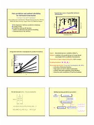
PENICILLIN G FED-BATCH FERMENTATION 25Step 6. Repeat Steps 1-5 with a new guess of SO in order to minimize J[u, XO].For the performance measure under consideration, equation (8), it can be easily shown (byusing (14) and (16)) that the stopping condition for this case is dP/dt(tr)=O, as could beexpected. In the case of a constraint on the control u and/or the state vector x, only someminor modifications are required, the algorithm itself remaining a two-dimensional search. Adetailed analysis of this algorithm in comparison with the algorithm proposed by Lim et al. l5together with a verification of all necessary conditions for optimality can be found inReference 4. The main difference from the algorithm of Lim et al. is that we do not make useof the costate variables, whatever the performance index under consideration.3.2. Simulation resultsWe now present some results obtained with the above computational algorithm. Weconcentrate on two specific values of the parameter B (i) B = lo-" as an approximation ofthe original Blackman-type kinetics (3) and (ii) the other extremal value B = krit = lo-', where~ ( p reduces ) to the Monod-type law (13).3.2.1. B = 10-". In the left plot of Figure 4 we have visualized the actions taken by theFor every SO the optimal switch time t2 has beencomputational algorithm for B= lo-''.calculated. As a consequence, we obtain the corresponding values for P(tr) and tr. Clearly, theoptimal couple (&*, t;) is the one which maximizes P(tr). Observe the quadratic behaviour ofP(tr) as a function of SO, so that there exists a unique optimal solution to this problem.Observe that there exists a lower limit Smin on the possible values for SO, corresponding totz = 0. In that case the complete initial state xo is on the singular hyperplane, so singularcontrol starts immediately. Note that SO = a corresponds to a complete batch fermentation:tr = t3 = tz, with u(t) = 0 for ali t. Even for values of SO in the neighbourhood of a, thecondition dP/dt = 0 is never met before t = t2. As a result, we can indeed apply the proposedcomputational algorithm to the whole possible range SO E [Smin, a]. A derived benefit is ofcourse that a good starting value for SO is not required for the algorithm to converge. Somenumerical values for the optimal control are summarized in Table 11. The right plot of Figure 4100 0.2 0.4 0.6 0.8 1 1.2 1.4 1.6 1.8 2s(w Id1.LO+Figure 4. B= lo-". Left plot: extremal values for P(tf), t2 and tf as functions of SO. Scaling: tJSO, rf/500,(P(tr) - 8150)/180. Right plot. optimal glucose feed rate and corresponding cell, glucose, product, T- and p-profiles.Scaling: c, x 300, c, x 5, q103, p x 100, r x 2 x lo4, u/300Time [h]
Page 1 and 2: OPTIMAL CONTROL APPLICATIONS & METH
Page 3 and 4: PENICILLIN G FED-BATCH FERMENTATION
Page 6 and 7: 18 J. F. VAN IMPE ETAL.~=o(lO-~). U
Page 8 and 9: PaPa20 J. F. VAN IMPE ETAL.The opti
Page 10 and 11: 22 J. F. VAN IMPE ETAL.XIO-43.53.0
Page 14 and 15: 26 J. F. VAN IMPE ET AL.Table 11. O
Page 16 and 17: 28 J. F. VAN IMPE ETAL.-11 -10 -9 4
Page 18 and 19: 30 J. F. VAN IMPE ET AL.--I 1.z 1.4
Page 20 and 21: 32 J. F. VAN IMPE ETAL.5.0 B im 150
Page 22: 34 J. F. VAN IMPE ET AL.3. Van Impe

Optimal control of the penicillin G fed-batch fermentation: An ...

You also want an ePaper? Increase the reach of your titles

Delete template?

Save as template?