Optimal control of the penicillin G fed-batch fermentation: An ...

More documents

Recommendations

Info

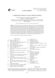
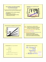
22 J. F. VAN IMPE ETAL.XIO-43.53.0 0.002 0.004 0.006 0.008 0.01 0.012 0.014 0.016 0.018 0.02PIlhlFigure 3. Dabes-type kinetics rh) for various values of parameter Bfamily of models - that is completely smooth within the given boundaries of the parameterB, thus assuring the continuity of afi/ax, for all i and j. Moreover, as BZO, we comearbitrarily close to the original model. In Figure 3 we show some members of the family (12)for different values of B. From the numerical point of view, setting B = lo-" in equation (12)is a very accurate approximation in simulating the original Blackman-type kinetics (3).Obviously, we can now determine the optimal control u*(B, t) for every B within the givenboundaries ]O,pcrit] using standard optimal control theory. For the original model -corresponding to B = 0 - we will make use of Conjecture 1.Observe that from a mathematical point of view the approximation of the piecewise smoothBlackman-type kinetics (3) can be done by any family of completely smooth curves thatconverges to the original kinetics. Clearly, the optimal control solution for the original kineticsis independent of this choice. However, from a biochemical point of view a sharp corner in7 at p = pcrit must be considered as a first approximation of real-life fermentation conditions.By using Dabes-type kinetics, each model of the sequence (.An) can be assigned a meaningfulinterpretation.3. OPTIMAL CONTROL USING THE MODIFIED MODEL3.1. Solution of the two-point boundary value problemThe given optimization problem can be formulated within the frame of the minimumprinciple l2*I3 as a two-point boundary value problem (TPBVP). The Hamiltonian Xfor thisproblem isThe adjoint vector X satisfies the following system of differential equations:
PENICILLIN G FED-BATCH FERMENTATION 23can be obtained by substituting equation (12) in equation (4) and calculating the implicitpartial derivatives with respect to XI and x4 respectively.The state equations (6) together with the costate equations (15) constitute a set of 2 x 4 firstorderdifferential equations. The required boundary conditions are as follows.(i) x~(0) and x3(0) are given.(ii) XI (0) and xq(0) are interrelated by equation (7).(iii) Since xl(0) and n(0) are not given explicitly, it can be shown that the followingcondition must be ~atisfied:~(iv) xq(tf) is given by equation (10).(v) X;(tf), i = 1, ..., 3, are given byXI@) + h(O)/Cs,in $(O) = 0or, using (8),(Xl(tf) XZ(tf) Xdtr))'=(O 0 -1)' (16)As stated in the minimum principle, an extremal control follows from the minimization of theHamiltonian .34? in (14) over all admissible control functions while satisfying the given TPBVP:min N(X*, A*, u) = s(x*, A*, u*)all admissible uNote that since all conditions are necessary conditions, we can only obtain extremol solutions(x*, X*, u*) which must be checked for optimality. Because the state equations (6) and the costindex (8) are time-invariant , the Hamiltonian .X' remains constant along an extremaltrajectory. Since the final time tf is free, we know that a'= 0.As already mentioned, the original kinetics (2)-(4) represent a degenerate case of afermentation process with monotonic specific growth rate p and non-monotonic specificproduction rate ?r - the corner point is a degenerate maximum - for which an efficientcomputational algorithm yielding the optimal control has been derived in Reference 4.However, the original model is only piecewise smooth, so this algorithm cannot be useddirectly because it requires the computation of the partial derivatives (up to second order) ofthe right-hand side of model equations (6) with respect to the state.We verify now that the computational algorithm can be used for any model with a specificproduction rate kinetics within the family of completely smooth curves (12). The optimalsolution using the original model is then obtained by considering the limitas stated in Conjecture 1.Iim u*@, t) 4 U*(B = 0, t)B>,OBecause the Hamiltonian .34? is linear in the control input u, the minimum principle fails toprovide the solution on any singular interval [ti, ti+l] where the function I,L remains zero. Ithas been shown4 that this problem is a singular problem of order two. In that case the singularcontrol can be calculated by solving
Page 1 and 2: OPTIMAL CONTROL APPLICATIONS & METH
Page 3 and 4: PENICILLIN G FED-BATCH FERMENTATION
Page 6 and 7: 18 J. F. VAN IMPE ETAL.~=o(lO-~). U
Page 8 and 9: PaPa20 J. F. VAN IMPE ETAL.The opti
Page 12 and 13: 24 J. F. VAN IMPE ETAL.for the cont
Page 14 and 15: 26 J. F. VAN IMPE ET AL.Table 11. O
Page 16 and 17: 28 J. F. VAN IMPE ETAL.-11 -10 -9 4
Page 18 and 19: 30 J. F. VAN IMPE ET AL.--I 1.z 1.4
Page 20 and 21: 32 J. F. VAN IMPE ETAL.5.0 B im 150
Page 22: 34 J. F. VAN IMPE ET AL.3. Van Impe

Optimal control of the penicillin G fed-batch fermentation: An ...

Create successful ePaper yourself

Delete template?

Save as template?