A dynamic thermal identification method applied to condutor ... - IEM

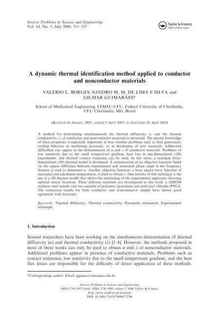
Inverse Problems in Science and EngineeringVol. 14, No. 5, July 2006, 511–527A dynamic thermal identification method applied to conductorand nonconductor materialsVALE´RIO L. BORGES, SANDRO M. M. DE LIMA E SILVA andGILMAR GUIMARA˜ ES*School of Mechanical Engineering, FEMEC/UFU, Federal University of Uberlaˆndia,UFU Uberlaˆndia, MG, Brazil(Received 10 January 2005; revised 8 April 2005; in final form 20 April 2005)A method for determining simultaneously the thermal diffusivity, , and the thermalconductivity, l, of conductor and nonconductor materials is presented. The precise knowledgeof these properties is especially important in heat transfer problems such as heat generation,cooling behavior in machining processes, or in developing of new materials. Additionaldifficulties can appear in the determination of and l of conductor materials. Problems oflow sensitivity due to the small temperature gradient, heat loss in one-dimensional (1D)experiments, and thermal contact resistance can be cited. In this sense, a transient threedimensional(3D) thermal model is developed. A minimization of an objective function basedon the square difference between experimental and numerical phase angle in the frequencydomain is used to determine . Another objective function, a least square error function ofmeasured and calculated temperatures, is used to obtain l. One novelty of this technique is theuse of a 3D thermal model that allows the optimizing of the experimental apparatus choosingoptimal sensor locations. Three different materials are investigated in this work: a AISI304stainless steel sample and two samples of polymers (polythene and polyvinyl chloride (PVC)).The estimation results for both conductor and nonconductor sample have shown goodagreement with literature.Keywords: Thermal diffusivity; Thermal conductivity; Parameter estimation; Experimentaltechnique1. IntroductionSeveral researchers have been working on the simultaneous determination of thermaldiffusivity () and thermal conductivity (l) [1–6]. However, the methods proposed inmost of these works can only be used to obtain and l of nonconductor materials.Additional problems appear in presence of conductive materials. Problems such ascontact resistance, low sensitivity due to the small temperature gradient, and the heatflux losses are responsible for the difficulty of direct application of these methods.*Corresponding author. Email: gguima@mecanica.ufu.brInverse Problems in Science and EngineeringISSN 1741-5977 print: ISSN 1741-5985 online ß 2006 Taylor & Francishttp://www.tandf.co.uk/journalsDOI: 10.1080/17415970600573700

A dynamic thermal identification method 513yzxφ 1 (t)Τ 1 (t)Τ 2 (t)Isol ated surfaceS 1bacIsolated surfaceFigure 2.3D thermal equivalent model.in the region R (0 < x < a, 0

514 V. L. Borges et al.model can be associated with the dynamic model given by equation (2). In this case,using the same procedure described in the one-dimensional (1D) case in the previouswork [10] the equivalent thermal model can be obtained as the convolution productin the frequency domain. 1 ð f Þ 2 ð f Þ¼G þ 12 ð f Þ 1ð f Þ ð6Þwhere the variable f indicates that Fourier transform was applied to the variables , ,and G þ 12. A comparison of equation (6) with equation (1) givesG þ 12 ðt Þ ¼hðt Þ ¼ ½ Gðx 1, y 1 , z 1 , t Þ Gðx 2 , y 2 , z 2 , t ÞŠ ð7ÞIt can be observed that as i (t) e i (t) are obtained by discrete measurements, Fouriertransforms can be performed numerically by using the Cooley–Tukey algorithms(Discrete Fast Fourier Transform) for these data [7]. Therefore, the equivalent thermalsystem to the dynamic system can be represented by:Zð f Þ¼hð f Þ¼ 1ðfÞ 2 ðfÞðfÞ 1¼ Yð f ÞXð f Þð8Þwhere the function Z( f ), also called impedance generalized, is equivalent to theresponse in frequency H( f ) defined by equation (2). Observing equations (4) it can beconcluded that the frequency response H( f ) is strongly dependent of the thermalproperties, which means:Hð f Þ¼ 1ð f Þ 2 ð f Þ¼ function ð, Þð9Þ 1 ð f ÞIt should be observed that the transformed impedance in the f–x plane is a complexvariable which in a polar form can be written byZð f Þ¼Hð f Þ¼Hð f Þ ej’ð f Þð10Þwhere jHj and ’ represent, respectively the modulus and the phase factor of H. Thephase factor can be written by’ð f Þ¼arctan g ½Im Hð f Þ=Re H ð f ÞŠ ð11Þwhere Re H( f ) and Im H( f ) are the real and imaginary parts of H.The phase of frequency response H( f ) and the time evolution of superficialtemperatures, T 1 (t), and T 2 (t) are the experimental data used for estimation of thermaldiffusivity and thermal conductivity respectively.2.2. Thermal diffusivity estimation: frequency domainThe fact that the phase factor is just a function of the thermal diffusivity is the greatconvenience of working in the frequency domain. The basic idea here is the observationthat the delay between the experimental and theoretical temperature is an exclusivefunction of . Therefore, the minimization of an objective function, S p , based on the

A dynamic thermal identification method 515difference between experimental and calculated values of the phase is used to determinethe thermal diffusivity. This function can be written asS p ¼ XNfi¼1ð’ e ðiÞ ’ t ðiÞÞ 2 ð12Þwhere ’ e and ’ t are the experimental and calculated values of the phase factor of Hrespectively. The theoretical values of the phase factor are obtained from theidentification of H( f ) by equation (11). In this case, the output Y( f ) is the Fouriertransform of the difference 1 (t) 2 (t) obtained by the numerical solution ofequations (4) using the finite volume method [11]. In fact, this procedure avoids thenecessity of obtaining an explicit and analytical model of H( f ).The values of will be supposed to be those that minimize equation (12). In thiswork, this minimization is done by using the golden section method with polynomialapproximation [12].2.3. Thermal conductivity estimation: time domainOnce the thermal diffusivity value is obtained, an objective function based on leastsquare temperature error can be used to estimate the thermal conductivity. In this case,there is no identification problem as just one variable is being estimated. Therefore, thevariable l will be supposed to be the parameter that minimizes the least square function,S mq , based on the difference between the calculated and experimental temperaturedefined byS mq ¼ Xsj¼1X ni¼1½ e ði, jÞ t ði, jÞŠ 2 ð13Þwhere e (i, j) is the experimental temperature and t (i, j) is the calculated temperature,n is the total number of time measurements and s represents the number of sensors.The optimization technique used to obtain l is also the golden section method withpolynomial approximation [12].3. Sensitivity analysisAlthough the thermal contact resistance and the low gradient problems do notrepresent any difficulties for non-metallic materials, they must be taken into accountin the presence of conductor materials. This section discusses both problems.Figure 3a presents the thermal contact resistance that can appear between sampleand sensors in a 1D model. Figure 3b presents the 3D alternative model to avoid thisproblem. Another advantage in a 3D model is the experimental flexibility allowing theoptimal location of the identification sensors.In 1D model, a high magnitude of heat flux (input) can be necessary to establisha thermal gradient high enough for the estimation process. Figures 4 and 5 presenta simulation using the same heat flux input. It can be observed that, while thetemperature gradient is situated in the region of the uncertainty of thermocouples

516 V. L. Borges et al.φ 1 (t)T 1 (t)φ 1 (t)T 2 (t)T 1 (t)T(x,y,z,t)y(a)T 2 (t)(b)zxThermocoupleElectrical resistance and heat transducerFigure 3. Experimental scheme for models (a) 1D and (b) 3D.(a)656055504540Temperature [°C]T1T2353025200 100 200 300Time (s)(b) 4038Temperature [°C]353330T128T22523200 200 400 600Time (s)Figure 4. Temperature evolution, T, for AISI304 sample (a) 1D model and (b) 3D model.(0.3 K) (figure 4a), the three-dimensional model produces a sufficient gradient toproperties estimation (figure 4b). Figure 5 presents the difference between the twotemperatures involved in each model as shown in figure 3.This fact can be better analyzed through a sensitivity analysis. Small and/orinaccurate values of temperature difference and heat flux signals produce lineardependence or low values. The linear dependence of two or more coefficients indicatesthat the parameters cannot simultaneously be estimated. Low values indicate thatthe estimation is strongly sensitive to the measurements uncertainty [6]. The sensitivity

(a) 0.5∆θ (°C)0.40.30.20.10.00 100 200 300Time (s)Figure 5.A dynamic thermal identification method 517(b)∆θ (°C)98765432100 200 400 600Time (s)Temperature difference, for AISI304 sample: (a) 1D model, and (b) 3D model.0.250.200.15Sensitivity coefficient0.100.050.00−0.05−0.10−0.15−0.20S T,aS T,l−0.250 10 20 30 40 50 60Time (s)Figure 6. Sensitivity coefficients for the 3D model to AISI304 sample.coefficients involved in this technique are defined as follows and presented infigures 6 and 7.S T, ¼ @TT @ ,S jHj, ¼ @ jHjjHj@S T, ¼ @TT @ , S ’, ¼ @’’ @ , S ’, ¼ @’’ @ ,and S jHj, ¼ jHj@ jHj@ð14Þ

518 V. L. Borges et al.(a)Sensitivity coefficient (S j,a )0.200.00−0.20−0.40−0.60−0.803D1DSensitivity coefficient, (S j,m )0.0100.0050.000−0.005−1.00−0.0100.000 0.003 0.005 0.008 0.010 0.00 0.05 0.10 0.15 0.20Frequency (Hz)(b)1D3DFrequency (Hz)Figure 7. Sensitivity coefficient of phase for 1D and 3D for the AISI304 sample (a) related to and(b) related to l.Heat flux inputFigure 8.Spatial temperature in a thin conductor sample.Figure 6 reveals a linear dependency of S T, and S T,l as shown by the symmetry. Thisfact indicates that both thermal properties cannot be estimated simultaneously in thetime domain justifying the use of frequency domain for the thermal diffusivityestimation.The sensitivity coefficients of phase related to the thermal diffusivity and thermalconductivity for 1D and 3D model are presented in figure 7.It can be observed in figure 7 that the values of the sensitivity of phase related to thethermal diffusivity are higher for the 3D model and there is no possibility to estimatethe thermal conductivity in frequency domain due to S ,l ¼ 0 for any frequency value.This fact reveals that the phase dependency with thermal diffusivity is unique andexclusive.Another advantage of using a 3D model is the possibility of estimating thermalproperties from a thin sample. In the 1D case, for conductor materials, it is very hard toobtain temperature gradients with values high enough to allow a good estimation as infigure 8. For a sample with thin thickness, it can be seen that no temperature variationin the direction y is observed. This fact makes the one-dimensional analysis unpractical.

A dynamic thermal identification method 5190.00−0.20−0.40Calibrated dataOriginal dataPhase (rd)−0.60−0.80−1.00−1.20−1.400.000 0.002 0.004 0.006 0.008Frequency (Hz)Figure 9.Phase factor subjected to the original and calibrated pair of input/output data.0.0140.0120.010Calibrated dataOriginal data⏐ Z ⏐0.0080.0060.0040.0020.0000.000 0.002 0.004 0.006 0.008Frequency (Hz)Figure 10. Modulus of Z for the original and calibrated pair input/output.Another important characteristic of the technique presented here is the very lowsensitivity of related to the amplitude of the signals X and Y. It means that theestimated value of the thermal diffusivity is insensitive to bias error, like uncertainty dueto poor calibration of thermocouples or heat flux transducers or both. This fact can bedemonstrated by verifying figures 9 and 10 which show the behavior of phase factor

520 V. L. Borges et al.and modulus due to the same input/output signals in both versions: original data,mVmV 1 , and calibrated data W m 2 / C.It can be observed in figures 9 and 10 that there are no changes in the phase factorwhile the modulus is strongly affected.4. Experimental4.1. Conductor material applicationIt can be observed that the boundary conditions present in the theoretical model mustbe guaranteed in the experimental apparatus. It means that the isolated condition at thereminiscent surface needs to be reached for the success of the estimation techniques.A good way to reach the isolation condition in a vertical direction is the use of asymmetric experiment apparatus. Figure 11 presents this scheme.13953ThermocoupleSample65Insulating materialElectrical resistanceHeat flux transducerInsulating materialSampleSample1010Symmetry lineSample65Dimensions in mmFigure 11.Schematic of experimental apparatus.

A dynamic thermal identification method 521The effect of no heat flux lateral loss is reached by placing insulating material such asexpanded polystyrene as shown in figure 11. Two AISI304 stainless steel samples wereused in a symmetric assembly, both with thickness of 10 mm and lateral dimensions of139 65 mm. The sample initially in thermal equilibrium at T 0 is then submitted toa unidirectional and uniform heat flux. The heat is supplied by a 318 electricalresistance heater, covered with silicone rubber, with lateral dimensions of 50 50 mmand thickness 0.3 mm. The heat flux are acquired by a transducer with lateraldimensions of 50 50 mm, thickness 0.5 mm, and constant time less than 10 ms.The transducer is based on the thermopile conception of multiple thermoelectricjunction (made by electrolytic deposition) on a thin conductor sheet [3]. Thetemperatures are measured using surface thermocouples (type k). The signals ofheat flux and temperatures are acquired by a data acquisition system HP Series 75 000with voltmeter E1326B controlled by a personal computer.Twenty independent runs were performed. In each of the experiments 1024 pointswere acquired, at time intervals of 0.54 s. The time duration of heating, t h , wasapproximately 120 s with a heat pulse generated at 90 V (DC).Figure 12 shows the evolution of the input/output normalized signals in functionof time for one of the experiments of AISI304 sample.Tables 1 and 2 present, respectively, the value estimated of and l for the AISI304stainless steel sample.In table 3 a summary of the simultaneous estimation of and l of the AISI304sample is presented. In this table, the value obtained for using the Flash method [13]and the value of l from Incropera and DeWitt [14] are also presented.An excellent agreement can be observed between the values of this work and theliterature for the thermal diffusivity and the thermal conductivity (error less than 2%).Figure 12.Input data of a typical run.

522 V. L. Borges et al.Table 1. Statistical data of the average value of (initial value of ¼ 1.0 10 6 m 2 s 1 ). (m 2 s 1 ) Initial S p Final S p (m 2 s 1 )3.762 10 6 20 1.16 10 3 4.0 10 8Table 2. Statistical data of the average value of l (initial value of l ¼ 10 W m K 1 ).l (W m K 1 ) Initial S p Final S p (m 2 s 1 )14.64 14700 18.3 3.1 10 1Table 3.Summary of and l for AISI304 sample.Thermal properties This work References [13,14] Error (%) 10 6 (m 2 s 1 ) 3.762 3.82 1.54l (W m K 1 ) 14.64 14.90 1.771210Temperature (°C)8642θ t1θ t2θ e1θ e200 50 100 150 200 250 300Time (s)Figure 13. Output of a typical run.These results show the potential of the method proposed here. The comparison betweenthe experimental and estimated temperatures for ¼ 3.76 10 6 m 2 s 1 andl ¼ 14.64 W m K 1 is shown in figure 13. In this figure a good agreement between thedata can be observed; the residuals are situated in the range of uncertainty measurementof thermocouples, that in this work is 0.3 K.

A dynamic thermal identification method 523Figure 14. Experimental apparatus used for determining and l.Table 4. Statistical data of the average value of (initial value of ¼ 1.0 10 8 m 2 s 1 ). (m 2 s 1 ) 10 7 Initial S p 10 2 Final S p 10 7 (m 2 s 1 ) 10 101.24 6.0 3.6 7.064.2. Nonconductor material applicationThe thermal identification technique can also be applied to nonconductor solidmaterials. In this case, a one-dimensional model can be used. This section presents someresults of and l estimation for two different polymers: polythene and polyvinylchloride (PVC). More details about the 1D model and its respective sensitivity analysiscan be found in [10].Two polymers samples were used, polythene and PVC, both with thickness of 50 mmand lateral dimensions of 305 305 mm. Figure 14 shows the experimental apparatuswhere at time t ¼ 0, the sample is in thermal equilibrium at T 0 . At this instant, thesample is submitted to a unidirectional and uniform heat flux on its upper surface.The heat is supplied by a 22 electrical resistance heater, covered with silicone rubber,with lateral dimensions of 305 305 mm and thickness 1.4 mm. The heat flux andtemperature are acquired using sensor and instruments with the same specification ofthat described here in the conductor material application.Fifty independent runs for PVC and twenty independent runs for polythene wererealized. For both samples 1024 points were taken. The time intervals, t, were 7.034 sfor PVC and 6.243 s for polythene. The time duration of heating, t h , was approximately150 s for PVC and 90 s for polythene with a heat pulse generated at 40 V (DC) forboth samples.Tables 4 and 5 present respectively the value estimated of and l for the fifty runsof PVC, with 99.87% confidence interval. In table 6 a summary of the simultaneousestimation of and l of the PVC sample is presented. In this table, the comparison withthe values obtained for by using the Flash method [14] and l by using the guardedhot plate method [15] presented errors of 3.22 and 3.30% for and l, respectively.In figure 15a a comparison between experimental and estimated phase factor ispresented. A very good agreement can be observed between them. Figure 15b shows theresiduals.

524 V. L. Borges et al.Table 5. Statistical data of the average value of l (initial value of l ¼ 0.01 W m K 1 ). (m 2 s 1 ) 10 7 l (W m K 1 ) Initial S mq 10 6 Final S mq 10 5 (W m K 1 )1.24 1.88% 0.152 1.351 5.91 4.9Table 6.Summary of and l for PVC sample. (m 2 s 1 ) 10 7 (m 2 s 1 ) 10 7 (FM) l (W m K 1 ) l (W m K 1 ) (HPM)1.24 1.88% 1.28 3.1% 0.152 1.1% 0.157(a)(b)Figure 15.Phase factor: (a) experimental and calculated data (b) residuals.The comparison between the experimental and estimated temperatures for ¼ 1.24 10 7 m 2 s 1 and l ¼ 0.152 W m K 1 is shown in figure 16a. Again a goodagreement between the data can be observed. It can be noted that the residualspresented in figure 16b are situated in the range of uncertainty measurement of

A dynamic thermal identification method 525(a)Temperature (K)(b)Figure 16.Temperature evolution: (a) experimental and calculated data and (b) residual.thermocouples, that in this work is 0.3 K. Table 7 presents a summary of thesimultaneous estimation of and l for the polythene sample with a confidence intervalof 99.87%. For this sample only the reference value for l obtained by NPL [15] ispresented.5. ConclusionIn this work we have proposed a technique to simultaneously estimate thethermal diffusivity and the thermal conductivity. The technique can be used in bothconductor and nonconductor solids. Two polymers and an AISI304 sample are used.The results have shown good agreement when compared with literature values for all

526 V. L. Borges et al.Table 7.Summary of and l for polythene sample estimation. (m 2 s 1 ) 10 7 l (W m K 1 ) l (W m K 1 ) (HPM) Error (%)2.14 1.15% 0.383 1.68% 0.389 1.57samples tested. The calculation of the phase factor numerically is one of the importantadvantages of the technique proposed here. This procedure allows the use of a 3Dtransient model and consequently its application to conductor material identification.The estimation of thermophysical properties of complex forms (such as a cutting tool) isa subject for future study.Nomenclaturef ¼ frequency (Hz)G ¼ Green’s function (m 2 KW 1 )H( f ) ¼ frequency response function (m 2 KW 1 )jHð f Þj ¼ modulus of frequency response functionIm(S xy ) ¼ imaginary component of the cross-spectral density function (K 2 )Re(S xy ) ¼ real component of the cross-spectral density function (K 2 )S mq ¼ objective function (K 2 )S ¼ phase objective function (rad 2 )S xx ¼ autoespectral density function of x(t) (K 2 )S yy ¼ autoespectral density function of y(t) (K 2 )S xy ¼ cross-spectral density function (K 2 )t ¼ time (s)T 0 ¼ initial temperature ( CX(t) ¼ input signal in time domain ( C)Y(t) ¼ output signal in time domain ( C)X( f ) ¼ input signal in frequency domain ( C)Y( f ) ¼ input signal in frequency domain ( Cx, y, z ¼ geometric variables (m)Z ¼ generalized impedance (m 2 KW 1 )Greek symbols ¼ thermal diffusivity (m 2 s 1 )l ¼ thermal conductivity (W m K 1 ) ¼ heat flux (W m 2 ) ¼ density (kg m 3 ) ¼ temperature difference ( C)( f ) ¼ phase angle (rad)Subscriptst ¼ relative to calculated datae ¼ relative to experimental data

A dynamic thermal identification method 527m ¼ relative to integer variables1 ¼ relative to the thermocouple 12 ¼ relative to the thermocouple 2.AcknowledgementsThe authors thanks CAPES, Fapemig and CNPq.References[1] Huang, C.H. and Yang, J.Y., 1995, An inverse problem in simultaneously measuring temperaturedependentthermal conductivity and heat capacity. International Journal of Heat and Mass Transfer, 38,3433–3441.[2] Dowding, K.J., Beck, J.V., Ulbrich, A., Blackwell, B. and Hayes, J., 1995, Estimation of thermalproperties and surface heat flux in carbon-carbon composite. Journal of Thermophysics and HeatTransfer, 9, 345–351.[3] Guimarães, G., Philippi, P.C. and Thery, P., 1995, Use of parameters estimation method in the frequencydomain for the simultaneous estimation of thermal diffusivity and conductivity. Review of ScientificInstruments, 66, 2582–2588.[4] Nicolau, V.P., Gu¨ths, S. and Silva, M.G., 2002, Medic¸ão da condutividade te´rmica e do calor especı´ficode materiais isolantes. ENCIT 2002, Brazil.[5] Lima e Silva, S.M.M., Ong, T.H. and Guimara˜es, G., 2003, Thermal properties estimation of polymersusing only one active surface. RBCM, 25, 9–14.[6] Beck, J.V. and Arnold, K.J., 1977, Parameter Estimation in Engineering and Science (New York: JohnWiley and Sons Inc.), p. 501.[7] Bendat, J.S. and Piersol, A.G., 1986, Analysis and Measurement Procedures, 2nd Edn (USA: Wiley-Intersience), p. 566.[8] Özisik, M.N., 1993, Heat Conduction, 2nd Ed (New York: John Wiley & Sons), p. 692.[9] Beck, J.V., Cole, K.D., Haji-Sheik, A., and Litkouhi, B., 1992, Heat Conduction Using Green’s Function(USA: Hemisphere Publishing Corporation), p. 523.[10] Borges, V.L., Lima e Silva, S.M.M., and Guimara¨es, G., 2004, A dynamic thermal identification method:part I – non conductor solid material. Inverse Problems, Design and Optimization Symposium (Brazil: Riode Janeiro).[11] Patankar, S.V., 1980, Numerical Heat Transfer and Fluid Flow (Washington, DC: Hemisphere PublishingCorporation), p. 197.[12] Vanderplaats, G.N., 1984, Numerical Optimization Techniques for Engineering Design (New York, USA:McGraw-Hill).[13] Lima e Silva, S.M.M., 2000, Experimental Technique Development for Determining Thermal PropertiesDiffusivity and Thermal Conductivity of Non-metallic Materials Using Only One Active Surface. DoctorateThesis (in portuguese), Uberlaˆndia, Brazil: Federal University of Uberlaˆndia, p. 115.[14] Incropera, F.P. and DeWitt, D.P., 1996, Fundamentals of Heat and Mass Transfer (New York: JohnWiley and Sons Inc), p. 886.[15] NPL, 1991, Certificate of calibration: thermal conductivity of a pair of polythene specimens, TechnicalReport No. X2321/90/021, England (unpublished).