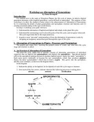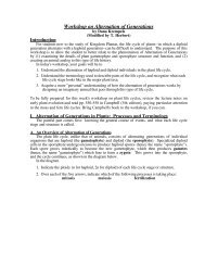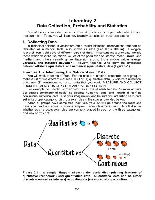
Laboratory 2 Data Collection, Probability and Statistics

Once the first member of the group has finished measuring and recording the ratiosof each group member, the other members of the group should each take a turnmeasuring and calculating the ratios. Each group member should measureindependently, and not look at the measurements taken by other group members. Youmay use the same method as your fellow group members, or you may choose adifferent method. But whatever protocol you select, be sure you use it consistently forall your measurements.Write down your own measured values in the table provided below:Group Sexmember (circle)Means MMMMFFFFn/aIndex fingerlength(cm)Ring fingerlength(cm)Index : ringRatioImportant note! When you calculate a ratio of two similar values, remember that theunits of the values--centimeters, in this case--cancel each other out. The ratio is thus adimensionless quantity.Does your mean differ from those calculated by your team members?Explain why or why not:When you have finished the above, select one group member's ratio values and turnthem in to your TA. The TA will list ratio values for each class member on theblackboard. From these data, you will calculate the mean ratio for the entire class.What is the mean index : ring finger ratio for your entire lab section?Is it different from the one you calculated from only your group members?Explain why or why not:Which mean ratio--your group's or the entire lab's--do you believe is closer to the trueparameter for all Homo sapiens, and why?2-3

You will complete a histogram of the ratios in the grid provided in Figure 2-1. The x axisshows the range of ratios, and the y-axis is the number of samples with any particularvalue on the x-axis. For example, if there were 10 students in your lab, and their ratioswere as follows:0.92, 0.95, 0.96, 0.96, 0.98, 0.97, 0.99, 1.01, 0.97, and 0.97Your histogram would look like this:10987654321.85 .86 .87 .88 .90 .91 .92 .93 .94 .95 .96 .97 .98 .99 1.0 1.01 1.02 1.03 1.04 1.05 1.06 1.07 1.08 1.09 1.1In the grid below, enter the index : ring finger ratio for every individual member of yourlab section. The number of squares blackened should equal the number ofmeasurements.28272625242322212019181716151413121110987654321.85 .86 .87 .88 .90 .91 .92 .93 .94 .95 .96 .97 .98 .99 1.0 1.01 1.02 1.03 1.04 1.05 1.06 1.07 1.08 1.09 1.1Figure 2-1. Frequencies of index : ring finger ratios in male and female studentsof BIL 151 section .2-4

Voila! You have created a frequency distribution! This is simply a representation ofhow often (i.e., how frequently) each value occurs in your sampled group (all your labcolleagues), how the values are distributed across all possible values, and around themean.What is the median of the entire lab section's ratios?What is the mode?Do these values differ from the median and mode of your four-person team?Explain any difference:III. Range, Variance and Standard DeviationAs you may recall, when you are studying some measurable aspect of a population(such as the index : ring finger length ratio), the degree of variation around the meanshould always be considered. In biological systems, there is almost always a great dealof variation around the mean of any given value. In many biological studies, theestimation of variances is as important, if not more important, than the mean.Measurements of dispersion around the mean include the range, variance andstandard deviation. The simplest of these is the range, which is defined as the highestvalue minus the lowest value. Unfortunately, the greater the sample size, the greaterthe range, and because it employs essentially only the two extreme values, a great dealof information about variation between those extremes is lost.More useful are the variance and standard deviation, which are measures ofdeviations from the mean. The variance (s 2 ) is calculated as_In which x is the mean, x is each individual value, and n is the sample size.The standard deviation (s) is the square root of the variance:Exercise 3. Calculating Range, Variance and Standard Deviationof your Frequency Distribution.What is the range of index : ring finger ratios for your lab section?What is the variance?2-5

What is the standard deviation?(Can you feel your IQ rising? Do not be alarmed. The symptoms will subside as soonas you go home and turn on the TV and watch "American Idol.")IV. Probability: What is meant by "expected results?"Probability calculations allow us to define the range of possible results of a seriesof trials, often in the form of a bell-shaped curve (a frequency distribution) representingthe likelihood of each possible result. In other words, these probability calculationsallow us to determine expected results from a particular series of events, be they aseries of coin flips, rolls of the dice, or carefully controlled experimental trials.When an investigator collects data from a subset of a population, s/he is interestedin determining whether some hypothesis about that population is true or false. Howdoes an investigator know whether any "unusual" results are significantly different fromwhat was expected, or whether such variation is due simply to random chance?Let's use the example of an event that has several possible outcomes, with each ofthose outcomes having an equal probability of occurring. For example, in any givenbirth, a single offspring will be genetically either male or female. There is a 1/2 chancethat it will be male and a 1/2 chance that it will be female.The probability (P) of any of those possible outcomes can be expressed as:a/n...wherea = the # of occurrences of the event in question andn = the total number chances a particular result has to occurFor example, because a die (that's the singular of dice) has six sides, there is alwaysa 1/6 chance on any roll that any given number (let's say a "6") will come up.When the probability of various events are known, scientific investigators canconsider their combined probabilities: the likelihood of two or more events happeningtogether. Let's illustrate with some actual games of chance.Exercise 4. Dice-o-Rama!At your lab station you will find several sets of dice. Work in pairs and use the diceto familiarize yourself with the three general rules of probability that form the basis of theSum Rule, the Product Rule and the Binomial Theorem.A. The Sum Rule: Dependent ProbabilitiesThe Sum Rule is used to determine the likelihood that either of two events occurswhen one precludes the other. In other words, each time a particular event has achance to occur, it's an "either/or" choice, such as flipping a coin or rolling a die once.Every time you flip a coin, it will come up either heads or tails--not both. Every timeyou roll a die, only one face will show, and no others. Every time a couple has a singlechild, it will be either genetically male or female--not both (no matter what you mightread in the Weekly World News).In the case of a single roll of a die, the probability of rolling a either a "one" or a "six"on any given roll can be expressed as the sum of the probabilities of rolling either a oneor a six. For example, the probability of rolling either a one or a six in one roll can becalculated asP = (a/n) 1 + (a/n) 62-6

Figure 2-2. Frequency distribution of rolls of "1" or "6" in trials of three rolls.Which of the four columns do you expect to have the highest frequency of "1" or "6"rolls?Why?Did your actual results confirm what you expected, given the known probability?Explain why or why not:When every pair of students has finished filling in a frequency distribution, your TAwill ask each team to display its graph. Do all the graphs reflect the same generalresults? Are there any that differ from the most probable outcome? Explain.Even though the expected result was one "1" or one "6" each time you rolled the diethree times, you probably got a distribution of all possible results in your trials. As youcan see, any set of three rolls could yield 0, 1, 2 or 3 incidences of a "1" or a "6". Thisdemonstrates that although a roll of "1" or "6" is probable in three rolls, it will not happenevery time. Variation is part of nature, and an important aspect of any scientific study.The larger the sample size, the more closely you will approximate the truepopulation parameter. If you were to pool all the rolls of your entire lab section,what do you think the frequency distribution would look like?When a subset of a population fails to show the expected result only because ofsmall sample size (as you may have seen in your die-rolling trials), the deviation fromthe expected is said to be due to random sampling error. Of greater interest to thescientist, of course, are deviations from the expected that occur despite an adequatesample size.B. The Product Rule: Independent ProbabilitiesThe Product Rule is used to determine the likelihood of two events occurring whenthe two possible results are independent of each other. Unlike the Sum Rule, which isused to determine "either/or" probabilities, the Product Rule is used to determine "and"probabilities, such as the results of flipping a coin, rolling a single die two times in a row,or having two female children in two births.The result of each roll of a die is independent of the next. The probability of rollingtwo particular numbers back-to-back in a specified order can be calculated as theproduct of each number's individual probability.Let's use the dice again. This time we'll calculate the probability that in rolling onedie twice in a row, you will roll a two, followed by a five. The probability is calculated asP = (a/n) 2 x (a/n) 5…where the subscripts indicate the probability of the chosen number.Given what you know about the probability of rolling a two or a five, calculate thelikelihood of rolling a two followed by a five in two back-to-back rolls of one die.Your answer: .You expect to get rolls of 2 followed by 5 in rolls of a single die.2-8

NOTE:The formula above is strictly for calculating the probability of rolling a 2 followed by afive. If you wanted to calculate the probability of simply rolling a 2 and a 5 in two rolls ofthe die, but do not want to specify the order, then each roll is considered one separateevent. You can get a combination of 2 and 5 by rolling first a 2, then a 5. Or you canget the same combination by rolling first a 5, then a 2. Either outcome (2 or 5) has a 1/6probability, so combining them will yield 1/6 x 1/6 = 1/36. But since there are two waysthis can happen, this probability must be doubled, making the total probability 2 x (1/6 x1/6) = 1/18. Have we lost you yet? You’ll thank us next time you’re in Vegas.Exercise 4b.Work in pairs. Each partner should roll two sets while the other partner recordsresults, then switch roles and repeat. When you're done, you and your partner will havea total of four sets of 36 rolls between you.On the following two pages, grids to record your number pairings are provided. Notethat each of your 36 rolls is paired with the roll immediately after it. For example, if yourset of rolls is:1 2 3 4 5 6 1 2 3 4 5 6 1 2 3 4 5 6 1 2 3 4 5 6 1 2 3 4 5 6 1 2 3 4 5 6Your pairings should be read as:1/2 2/3 3/4 4/5 5/6 6/1 1/2… and so forth.On the following four pages are grids for four sets of 36 rolls. Each page has a tablewith 36 squares for you to enter the number that comes up on each individual roll.When you have finished your four sets, note how many times you got a sequence of 2followed by 5.Set #1: Enter the number rolled in each of your 36 attempts:Number of times you got 2 followed by 5 in set #1:Set #2: Enter the number rolled in each of your 36 attempts:Number of times you got 2 followed by 5 in set #2:Set #3: Enter the number rolled in each of your 36 attempts:Number of times you rolled 2 followed by 5 in set #3:Set #4: Enter the number rolled in each of your 36 attempts:Number of times you rolled 2 followed by 5 in set #4:Once everyone is done, your TA will ask each pair to tell the rest of the class outloud how many rolls of 2 followed by 5 they got in each set. Label the axes of Figure 2-2-9

3 appropriately with independent (number of 2/5 sequences per set of 36 rolls) anddependent (frequency of number of 2/5 sequences per set of 36 rolls) variables.Record these values in Figure 2-3 by blackening the appropriate square as yourclassmates call out their results. When finished, the figure will be a frequencydistribution of how often a roll of 2 followed by 5 occurred in all class trials.35343332313029282726252423222120191817161514131211109876543210 1 2 3 4 5 6 7 8 9 10 11 12 13 14 15 16 17 18 1o 20 21 22 23 24 25 26 27 28 29 39 31 32 33 34 35Number of rolls of [2 followed by 5] in sets of 36 individual rolls of a dieFigure 2-3. Frequency distribution of 2/5 sequences in sets of 36 rolls.Do the pooled data from the entire class approximate what was expected? Explain.C. The Binomial Theorem: Multiple Independent ProbabilitiesThe Binomial Theorem is used to generate the probability of two events occurringtogether over multiple trials when each event has an independent probability ofoccurring. Let's say we have two alternative events, X and Y.The probability of X is p.The probability of Y is q.n = the number of trials in which either X or Y can occur.2-10

s = the number of times event X occurs in your trialst = the number of times event Y occurs in your trials(Recall that, by definition, p + q = 1.0 and s + t = n.)Let's say that you plan to perform a series of trials in which either result X or result Ycan occur. The probability that X will occur s times and Y will occur t times can becalculated with the following equation(recall: ! is the symbol for factorial. For example, 10! = 1x2x3x4x5x6x7x8x9x10)Exercise 4c.Work in pairs. At your station you will find a container full of colored, flat marbles.Each container is an egg case laid by a female member of a rare species known asSilicus vitreosus. (Humor us.) The eggs, which bear a striking resemblance to flatmarbles, come in two colors. The blue eggs will hatch out as males, and the pink eggswill hatch out as females. (PLEASE DON'T LOSE ANY MARBLES OR ADD ANYFROM OTHER CONTAINERS!)Because sex in Silicus vitreosus is determined by X and Y chromosomes, with XXbeing female and XY being male, there is a 50% probability (all other things being thesame) that any given egg will be male or female.Let's consider the laying of a female egg as event X, and the laying of a male egg asevent Y. This means that in any given clutch of eggs, the number of females is s, andthe number of males is t. There is a 0.5 chance that an egg will be female, and a 0.5chance that it will be male.Let's hatch some eggs! While one partner holds the container, the other shouldclose his/her eyes and randomly draw out 10 marbles. Okay, it's safe to open youreyes. How many of each color did you get? What are the sexes of the babies?# of females (Event X): (this is your value for s)# of males (Event Y): (this is your value for t)Plug your observed values into the binomial equation and calculate P.What was the probability of your observed result?Which combination of colors in a 10-egg clutch do you think would have the highestprobability of occurring, and what IS that probability?As before, there is a particular probability associated with every combination of colors inany given clutch. Also as before, the occurrence of each color combination could beplotted along a frequency distribution similar to the ones you did for the finger ratios anddice rolls. We will not create another frequency distribution for this example. However,you should feel confident that you could create one, should the need arise.If so, what would be the appropriate units of the x axis?What about the y-axis?2-11

V. Hypotheses and Statistical TestsThe Scientific Process begins with three important steps:1. The observation of some phenomenon that elicits a question/poses a problem.2. The formulation of competing, testable hypotheses about that phenomenon3. The prediction of all possible outcomes of experiments designed to test eachhypotheses.For example, as you wander in a field of wildflowers, you notice that individuals of aspecies of yellow poppy have two distinct morphologies, one with spines and onewithout. You also noticed that the individuals with spines were far more numerous thanthe smooth individuals. You might wonder whether there was a reason for thedifference in their numbers, and ask whether the spiny individuals were better able todeter herbivores with their spines than the smooth individuals. There's your question.The next step is to formulate a testable null hypothesis, such as, "There is nodifference in herbivore damage between the spiny and smooth individuals." Youralternative hypothesis would be that there is a difference. In this case, the latter is yourprediction as well as your hypothesis of interest.Before you continue, review Appendix 2 and be confident you know the meanings ofinductive and deductive reasoning, null and alternative hypotheses, one-tailed andtwo-tailed hypotheses, and the precise definitions of hypothesis and theory.Statistical Tests and Probability DistributionsProbability calculations similar to those you did with the dice and marbles form thebasis of one of the scientist's most important tools: the statistical test. Once datahave been collected, it's not enough to merely "eyeball" them and say, "Eeyup. This isdifferent from what we expected! Something weird is going on here!"Instead, investigators use statistics calculated from their data sets to determine thelikelihood that their results are significantly different from the expected results. Over thedecades, many different probability distributions have been devised bymathematicians, each one appropriate for different types of data.Enough statistical tests and their associated probability distributions have beeninvented to fill many textbooks. Some of these, such as the Chi-square test, theStudent t-test, the Analysis of Variance (ANOVA), the Mann-Whitney U test and theFisher's exact test may sound familiar to you. The specific probability distribution andstatistical test appropriate in a given situation depend upon the type of data collected.One oft-utilized probability distribution is the t-distribution, used to determinewhether there is a significant difference between the (continuous numerical) means oftwo groups under study. To make a very long and complex story short, an investigatorcan use the mean, variance, and standard deviation of his/her data sets to calculate a t-statistic. Every possible t-statistic is linked to a certain probability that the data used tocalculate it differ because of some factor other than random chance.Exercise 5. The Student t-test: A tool for determining whetherthere is a significant difference between two meansThe Student t-test can be used to determine whether a difference between twomeans is significant. These means may be calculated from observations that are eitherpaired (as when individuals in a single group are subjected to "before and after"2-12

measurements, and data points are paired for each tested individual) or independent(as when individuals in two similar sample populations are measured, but eachindividual in each sample population is measured only once). Slightly differentcalculations of the t-statistic must be used in each case.Work in groups of four. Within each group, one pair of students will measure 30marbles and calculate their mean volume with one method, and the other pair willmeasure the same 30 marbles, but use a different method. There is more than one wayto calculate the volume of solid objects, and because we know you're tired, we'll clueyou in on a couple. But feel free to devise your own method if you're full of caffeine andfeeling creative.Method 1. Geometric calculation.Glass marbles are ostensibly spherical. If you can measure the diameter of themarble, you can calculate its volume with the old standard formula4/3 (π r 3 )…where π = 3.14 and r is the radius of the sphere. Millimeter rulers and calipers areavailable for you to use, and you may decide which you prefer. Report your results incubic centimeters (cm 3 , or cc).Method 2. Volume displacement.Glassware appropriate for measuring volume also is available at each lab table. Byfilling a graduated cylinder with a known volume of water, adding a marble and thendetermining the change in volume…well, it doesn't get much simpler. There are severalsizes and types of glassware. We'll leave it up to you to decide the details of how toobtain the most accurate measurements. Report your results in cm 3 . (Note that onemilliliter (ml) is equal to one cubic centimeter (cc).)Before you begin your measurements, answer the following:1. What is your null hypothesis (there may be more than one reasonable one.)?2. What is your alternative hypothesis?3. Do you predict that the two different measurement methods will yield the samevolume for each of your 30 marbles? .If you were measuring two sets of 30 similar marbles with the two methods, themeans of your two sample populations would be independent of one another, as asingle measurement is made on each individual. However, you will essentially beperforming "before" and "after" measurements of a single marble with two differentmethods. This means that the two values you attain will not be independent of oneanother, and are said to be paired.In a paired sample t-test, the separate means of two sample populations is notmeasured. Instead, you will calculate the difference between your first measurementand your second measurement on the same individual, and use this to calculate your t-statistic. The difference between your first and second measurements is represented_as d, and the mean of all your individual differences as d.2-13

The standard deviation and variance are calculated as you did them before, butsubstituting d and d for x and x in the equations you used in the first exercise. Thus, tocalculate the variance of your paired samples, you will use the following equation:To calculate the standard deviation, take the square root of the variance.Measure the marbles one at a time with Method #1, enter the volume in Column 2 ofthe grid provided, and then pass the same marble to your partner pair, who will measureit with Method #2, and enter the volume in Column 3._1. Calculate the mean difference in volume (d) from the data in Column 4:2. Calculate the variance of the differences in volume (s d 2 ).3. Calculate the standard deviation (square root of (s d 2 )):You're now almost ready to plug these values into the t-test for paired samples. Thelast thing you must do is to determine the number of independent quantities in yoursystem, or degrees of freedom.4. The degrees of freedom determine the significance level tied to every possible valueof a statistic (such as the t-statistic). The degrees of freedom is the number of datapoints that are free to vary without changing the test statistic, and this changesdepending on the type of statistic you are calculating. For the paired sample t-test,df = (n - 1)...where n is the number of independent quantities in your system.samples, n = the number of pairs in your system. In this case, n = 30.For pairedYour team of four should now calculate a t-statistic for the difference between yourtwo means, and use this to determine whether the difference between them issignificant. Use the following equation for the paired sample t-test:...where n is the number of pairs.What is the value of your t-statistic?2-14

Marble #123456789101112131415161718192021222324252627282930TOTALVolume in cc(Method I)Volume in cc(Method 2)Difference in Volume(d)|column 2 - column 3|VI. Probability and significanceThe term "significant" is often used in every day conversation, yet few people knowthe statistical meaning of the word. In scientific endeavors, significance has a highlyspecific and important definition. Every time you read the word "significant" in this book,know that we refer to the following scientifically accepted standard:The difference between an observed and expected result is said to be statisticallysignificant if and only if:Under the assumption that there is no true difference, theprobability that the observed difference would be at least as largeas that actually seen is less than or equal to 5% (0.05).Conversely, under the assumption that there is no true difference,the probability that the observed difference would be smaller thanthat actually seen is greater than 95% (0.95).2-15

Once an investigator has calculated a t-statistic, s/he must be able to drawconclusions from it. How does one determine whether deviations from the expected(null hypothesis) are significant?As mentioned previously, depending upon the degrees of freedom, there is aspecific probability value linked to every possible value of the t-statistic. Thus, everypossible t statistic indicates a certain probability that the data used to calculate it varysignificantly from the expected. Mathematical computation of probability distributions foreach statistical test is extremely complex. Fortunately, tables of probability (P) values atvarious degrees of freedom for each statistical test have been created for us by noblemathematicians (or actually, noble computer jockeys typing in the forumlae themathematicians have devised).Exercise 6. Determining the significance level of your t-statisticNow that you have calculated a t-statistic for your two sets of marble measurements,you must try to interpret what this statistic tells you about the difference between the twomethods. Is the difference significant, suggesting that there is something other thanchance causing the variation in volume yielded by each method? The answer lies in thetable of critical values for the t-statistic, part of which is illustrated in Table 2-2.1. Locate the appropriate degrees of freedom in the far left column.2. Look across the df row to find a t value closest to the one you obtained.3. If the exact value does not appear on the table, note the two t values which mostclosely border your value, or the single value that is either greater or smaller thanyour value.4. Find the P value(s) that correspond to your bordering values, and enter them in theappropriate space(s) below:> P >If the P value associated with your t-statistic is less than (or equal to) 0.05, there isless than 5% probability that chance deviations could have resulted in a mean volumedifference as great or greater than that actually observed. Thus there is a 95%probability that chance deviations could have resulted in a mean volume differencesmaller than that actually observed. If this is the case, you must reject your nullhypothesis and accept your alternative hypothesis.(Alternatively, for a "quick and dirty" P value, just find the t-statistic associated withP = 0.05 at your df. If the calculated t-statistic is larger than the one from the table,reject your null-hypothesis.)Judging from your P value, should you accept or reject your null hypothesis?Briefly explain WHY you believe your statistic indicated that you should reject or fail toreject your null hypothesis.2-16

Do you believe your results to be an accurate reflection of true population values?Support your contention, either way.Table 2-2. Table of critical values for the two-sample t-test. The P levels (0.05)indicating rejection of the null hypothesis are shown in bold for both one-tailed andtwo-tailed hypotheses. (From Pearson and Hartley in Statistics in Medicine by T.Colton, 1974. Little, Brown and Co., Inc. publishers.)2-tail --> 0.10 0.05 0.02 0.01 0.0011-tail --> 0.05 0.02 0.01 0.005 0.0005df1 6.314 12.706 31.821 63.657 636.6192 2.920 4.303 6.965 9.925 31.5983 2.353 3.182 4.541 5.841 12.9414 2.132 2.776 3.747 4.604 8.6105 2.015 2.571 3.365 4.032 6.8596 1.934 2.447 3.143 3.707 5.9597 1.895 2.365 2.998 3.499 5.4058 1.860 2.306 2.896 3.355 5.0419 1.833 2.262 2.821 3.250 4.78110 1.812 2.228 2.764 3.169 4.58711 1.796 2.201 2.718 3.106 4.43712 1.782 2.179 2.681 3.055 4.31813 1.771 2.160 2.650 3.012 4.22114 1.761 2.145 2.624 2.977 4.14015 1.753 2.131 2.602 2.947 4.07316 1.746 2.120 2.583 2.921 4.01517 1.740 2.110 2.567 2.898 3.96518 1.734 2.101 2.552 2.878 3.92219 1.729 2.093 2.539 2.861 3.88320 1.725 2.086 2.528 2.845 3.85021 1.721 2.080 2.518 2.831 3.81922 1.717 2.074 2.508 2.819 3.79223 1.714 2.069 2.500 2.807 3.76724 1.711 2.064 2.492 2.797 3.74525 1.708 2.060 2.485 2.787 3.72526 1.706 2.056 2.479 2.779 3.70727 1.703 2.052 2.473 2.771 3.69028 1.701 2.048 2.467 2.763 3.67429 1.699 2.045 2.462 2.756 3.65930 1.697 2.042 2.457 2.750 3.6462-17

VII. Erroneous ConclusionsThere is always the secret dread in the heart of any scientist that his/her datawere not collected properly, that the sample size was too small, or there wassome other confounding problem that caused the data to yield an answer thatdoes not reflect reality. In such cases, the P value associated with yourcalculated statistic might wrongly lead you to reject the null hypothesis if it isactually true, or perhaps fail to reject the null hypothesis if it is false.Type I Error: The mistaken rejection of a null hypothesis that is actually true.Type II error: The mistaken failure to reject a null hypothesis that is false.As you might intuitively know, a type I error can be more damaging than a type IIerror. For example, if a pharmaceutical company mistakenly is led to believe thata new drug causes a significant improvement in a medical condition, when itactually does not, it could cost not only tremendous amounts of money, but evenlives.Type II errors are most common when the sample size is too small, and arethus more easily corrected than type I errors.An experiment should never be considered 100% foolproof. Therefore, Inscience--as in all endeavors--honesty is of paramount importance. Experimentalresults do not always confirm predictions. Data manipulation or failure toaccurately report results constitutes intellectual dishonesty. Science is thepursuit of fact, not the pursuit of supporting pet hypotheses that might be wrong.2-18