Saad A. Manaa

An Approximate Solution to The Newell-Whitehead Equation by …∞u= ∑ un(8)n=0and the nonlinear term Nu, assumed to be analytic function f(u), is decomposed asfollows:∞Nu fu ( ) A ( u , u ,..., u )(9)= =∑ n 0 1n=0nwhere A n are the appropriate Adomian's polynomials. These A n polynomials depend onthe particular nonlinearity and these A n Adomian polynomials are calculated by thegeneral formula1 ⎡n ∞d ⎡ ⎛ kA ( u0, u1,..., u ) = ⎢ ⎢N λn! λ⎜∑un ⎢⎣d⎣ ⎝ k=0n n k⎞⎤⎤⎟⎥⎥⎠⎦⎥⎦λ =0Substituting eq. (8) and eq. (9) into eq. (5) gives∞ ∞ ∞− − −∑ =Φ+ 1 − 1 ∑ −1n n ∑ nn= 0 n= 0 n=0, n ≥ 0 (10)u L g L R u L A (11)Each term of series (8) is given by the recurrence relationu0−=Φ+ 1L gu L Ru L A−−=− 1 −11 0 0−−=− 1 −12 1 1−−=− 1 −13 2 2u L Ru L Au L Ru L Au::−1 =−L Ru−1− L A (12)n n−1 n−1where An are the special Adomian polynomials or equivalentlyϕSo, the practical solution for the n-term approximation is,nn−∑ 1i=0... (13)= u , n ≥1(14)iand the exact solution is173

Saad A. Manaa∞u= limϕn=∑u i(15)n→∞i=03. The Adomian decomposition method applied to Newell-Whitehead modelThe nonlinear wave equation with dissipation and nonlinear transport termis given as: [15], [16]Where are distinct real numbers and , are constants.For, Eq. (16) reduces to the nonlinear reaction- diffusion formfor different choices of the parameters a1, a2, a3 Eq. (17) reduces to the well knownnonlinear reaction diffusion equations appearing in many different branches ofsciences: when we get the Newell-Whitehead equation [20]∂u2= ∆u+ u(1− u )∂t( t,x)∈(0,∞)× Ωwith the initial and boundary conditionsu( x,0)= u0( x),x∈ Ωu(x,t)= 0, t > 0 , x = 0 and∂u= 0∂xat x = 0 andx = L.x = L(16)(17)(18)(18a)which arises after carrying out a suitable normalization in the study of thermalconvection of a fluid heated from below. Considering the Perturbation from a stationarystate, the equation describes the evolution of the amplitude of the vertical velocity if thisis a slowly varying function of time t and position x.The equation (18) written in an operator formLu= u + u − N(u)(19)txxwhere ∂3L t= and N ( u)= u is nonlinear term. Applying the inverse operator to the∂ tequation (19) and using the initial data (18a) yields−1−1−1u(x,t)= u ( x)+ L u + L u − L N()(20)0 xxuThe ADM suggests the solution u( x,t)componentsbe decomposed by infinite series of= ∑ ∞ u ( x,t)un(x,t)(21)n=0and the nonlinear operator N(u) by the infinite series of the Adomian polynomials= ∑ ∞ N ( u)A n(22)n =0The first four components of Adomain polynomials according to (13) read174

An Approximate Solution to The Newell-Whitehead Equation by …From eq. (21) and eq. (22), the iterates are determined by the following recursive way:u0= u0(x)(24)−1−1un= L ( ∆un−1+ un−1)− L ( An−1),n ≥ 1.The decomposition method provides a reliable technique that requires less work ifcompared with traditional techniques.4. Application and Numerical ResultsTo give a clear overview of the methodology, the following example will bediscussed. All the results are calculated by using the MATLAB 7.4 software.Consider the Newell-Whitehead equation [11]∂u= ∆u+ u(1− u∂twith the initial conditions2)(0..5( 2a) x)( −0.5(2a) x)a c1e − c2eu ( x,0)= −(25)(0.5( 2a) x)( −0.5(2a) x)b ( c e + c e + 1)And exact Solutionu(x,t)= −ab1( c e1c1e(0.5( 2a) x)2(0..5( 2a) x)+ c2e− c2e( −0.5(2a) x)( −0.5(2a) x)+ c3e( −3 / 2) a tSubstitution the initial condition eq. (25) into eq. (24) and using eq. (23) tocalculate the Adomian polynomials, yields the following recursive relation)(23)u0= −ab( cce(0..5( 2a) x)1(0.5( 2a) x)1eWe will takeseries are given by:− c e+ c( −0.5(2a) x)2( −0.5(2a) x)2e+ 1)(26). The first few terms of the decomposition(27)175

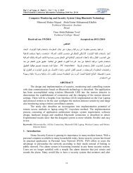
Saad A. Manaaother components are determined similarly (we will use four).Substituting relations (27) into recursive relation (21) yields+0-0.1-0.2AdomaimExact(28)-0.3-0.4u(x,t)-0.5-0.6-0.7-0.8-0.9-10 5 10 150 ≤ x ≤ 15 , t=0.5Fig.1: Comparison of exact and Adomain solution for t=0.50-0.1AdomaimExact-0.2-0.3-0.4u(x,t)-0.5-0.6-0.7-0.8-0.9-10 5 10 150 ≤ x ≤ 15 , t=1.0Fig.2: Comparison of exact and Adomain solution for t=1.0176

An Approximate Solution to The Newell-Whitehead Equation by …0-0.2AdomaimExact-0.4-0.6u(x,t)-0.8-1-1.2-1.40 5 10 150 ≤ x ≤ 15 , t=1.5Fig.3: Comparison of exact and Adomain solution for t=1.5Table 1: Comparison of the exact and Adomain decomposition solutionsAdomainDecompositionu(x,t)ExactSolutionu(x,t)AbsoluteErrorAdomainDecompositionu(x,t)ExactSolutionu(x,t)AbsoluteErrorAdomainDecompositionu(x,t)ExactSolutionu(x,t)AbsoluteError0≤x≤15 and t=0.5 10 -3 × 0≤x≤15 and t=1.0 0≤x≤15 and t=1.5X=0.0 0.0000 0.0000 0.0000 0.0000 0.0000 0.0000 0.0000 0.0000 0.0000X=0.5 -0.2772 -0.2778 0.5581 -0.2991 -0.3073 0.0082 -0.2869 -0.3235 0.0365X=1.0 -0.5118 -0.5128 0.9418 -0.5462 -0.5594 0.0132 -0.5274 -0.5844 0.0570X=1.5 -0.6848 -0.6858 0.9834 -0.7222 -0.7352 0.0130 -0.7078 -0.7611 0.0533X=2.0 -0.8008 -0.8015 0.7105 -0.8365 -0.8451 0.0086 -0.8349 -0.8674 0.0325X=2.5 -0.8745 -0.8748 0.3278 -0.9065 -0.9097 0.0032 -0.9182 -0.9272 0.0089X=3.0 -0.9203 -0.9203 0.0144 -0.9476 -0.9467 0.0009 -0.9678 -0.9597 0.0080X=3.5 -0.9487 -0.9485 0.1685 -0.9710 -0.9679 0.0031 -0.9939 -0.9773 0.0166X=4.0 -0.9664 -0.9662 0.2401 -0.9840 -0.9802 0.0038 -1.0056 -0.9869 0.0187X=4.5 -0.9777 -0.9774 0.2428 -0.9911 -0.9874 0.0037 -1.0096 -0.9922 0.0174X=5.0 -0.9850 -0.9848 0.2127 -0.9950 -0.9919 0.0031 -1.0098 -0.9952 0.0145X=5.5 -0.9898 -0.9896 0.1723 -0.9971 -0.9946 0.0025 -1.0085 -0.9970 0.0115X=6.0 -0.9930 -0.9928 0.1330 -0.9983 -0.9964 0.0019 -1.0068 -0.9981 0.0087X=6.5 -0.9952 -0.9951 0.0997 -0.9990 -0.9976 0.0014 -1.0052 -0.9987 0.0065X=7.0 -0.9966 -0.9966 0.0732 -0.9994 -0.9983 0.0010 -1.0039 -0.9992 0.0047X=7.5 -0.9977 -0.9976 0.0530 -0.9996 -0.9988 0.0007 -1.0028 -0.9994 0.0034X=8.0 -0.9984 -0.9983 0.0380 -0.9997 -0.9992 0.0005 -1.0020 -0.9996 0.0024X=8.5 -0.9989 -0.9988 0.0271 -0.9998 -0.9994 0.0004 -1.0015 -0.9997 0.0017X=9.0 -0.9992 -0.9992 0.0192 -0.9999 -0.9996 0.0003 -1.0010 -0.9998 0.0012X=9.5 -0.9994 -0.9994 0.0136 -0.9999 -0.9997 0.0002 -1.0007 -0.9999 0.0009X=10.0 -0.9996 -0.9996 0.0096 -0.9999 -0.9998 0.0001 -1.0005 -0.9999 0.0006X=10.5 -0.9997 -0.9997 0.0068 -1.0000 -0.9999 0.0001 -1.0004 -0.9999 0.0004X=11.0 -0.9998 -0.9998 0.0048 -1.0000 -0.9999 0.0001 -1.0003 -1.0000 0.0003X=11.5 -0.9999 -0.9999 0.0033 -1.0000 -0.9999 0.0000 -1.0002 -1.0000 0.0002X=12.0 -0.9999 -0.9999 0.0024 -1.0000 -1.0000 0.0000 -1.0001 -1.0000 0.0001X=12.5 -0.9999 -0.9999 0.0017 -1.0000 -1.0000 0.0000 -1.0001 -1.0000 0.0001X=13.0 -1.0000 -1.0000 0.0012 -1.0000 -1.0000 0.0000 -1.0001 -1.0000 0.0001X=13.5 -1.0000 -1.0000 0.0008 -1.0000 -1.0000 0.0000 -1.0000 -1.0000 0.0001X=14.0 -1.0000 -1.0000 0.0006 -1.0000 -1.0000 0.0000 -1.0000 -1.0000 0.0000X=14.5 -1.0000 -1.0000 0.0004 -1.0000 -1.0000 0.0000 -1.0000 -1.0000 0.0000X=15.0 -1.0000 -1.0000 0.0003 -1.0000 -1.0000 0.0000 -1.0000 -1.0000 0.0000It is clear from the figures (1-3) and the table that Adomain decompositionmethod is so accurate and converging to the exact solution.177

Saad A. Manaa5. ConclusionsThe Adomain decomposition method is effective and powerful method forsolving nonlinear partial differential Newell-Whitehead equations. The important part ofthis method is calculating Adomain polynomials for nonlinear operator.Acknowledgements: Words would not be enough to express my deep feeling ofgratitude and immense indebtedness to my wife for her continuous support andencouragement on this work.178

An Approximate Solution to The Newell-Whitehead Equation by …REFERENCES[1] Abbasbandy S., "A numerical solution of Blasius equation by Adomian’sdecomposition method and comparison with homotopy perturbation method",Chaos Solitons Fract 2007; 31:257–60.[2] Abbasbandy S., "Extended Newton’s method for a system of non-linearequations by modified Adomian decomposition method", Appl Math Comput2005; 170:648–56.[3] Adomian G., "An analytical solution of the stochastic Navier–Stokes system",Found Phys 1991; 21(7):831–43.[4] Adomian G., "Solving frontier problems of physics: the decomposition method",Boston: Kluwer Academic Publishers; 1994.[5] Adomian G., "Nonlinear Stochastic Operator Equations", Academic Press,Orlando, 1986.[6] Adomian G., "A review of the decomposition method in applied mathematics", JMath Anal. Appl 1988;135:501–44.[7] Adomian G., "Stochastic Systems", Academic Press, New York, 1983.[8] Allan FM, Syam MI., "On the analytic solutions of the non homogeneousBlasius problem", J. Comput Appl Math. 2005.[9] Chang MH., "A decomposition solution for fins with temperature dependentsurface heat flux", Int J Heat Mass Transfer 2005; 1819:24-48.[10] Chiu CH, Chen CK., "A decomposition method for solving the convectivelongitudinal fins with variable thermal conductivity", Int J Heat Mass Transfer2002; 45:2067–75.[11] Cicogna, G., “Weak” symmetries and adopted variables for differentialequations", Int. J. Geometric Meth. Modern Phys., Vol. 1, No 1–2, pp. 23–31,2004.[12] Hashim I., "Adomian decomposition method for solving BVPs for fourth-orderintegro- differential equations", J Comput Appl Math 2006; 658:64-193.[13] Hashim I., "Comments on A new algorithm for solving classical Blasiusequation", J Comput Appl Math 2005; 182:362–71.[14] Kaya D, Yokus A., "A decomposition method for finding solitary and periodicsolutions for a coupled higher-dimensional Burgers equations", Appl MathComput 2005; 164:857–64.[15] Kechil, S.A. and Hashim I., "Non-perturbative solution of free-convectiveboundary-layer equation by Adomian decomposition method ", Phys Lett A2007; 363:110.179

Saad A. Manaa[16] Newell A.C. and Whitehead J.A. Whitehead, "Finite bandwidth, _nite amplitudeconvection", J. Fluid Mech. 38 (1969), 279-303.[17] Pamuk S., "Solution of the porous media equation by Adomian’s decompositionmethod", Phys Lett A 2005; 344:184–8.[18] Wang L., "A new algorithm for solving classical Blasius equation", Appl MathComput; 2004; 157:1–9.[19] Wazwaz AM., "Approximate solutions to boundary value problems of higherorder by the modified decomposition method", Comput Math Appl 2000; 40(6–7): 679–91.[20] Wazwaz AM., "The decomposition method applied to systems of partialdifferential equations and to the reaction–diffusion Brusselator model", ApplMath Comput 2000; 110(2–3):251–64.[21] Wazwaz AM., "The modified decomposition method applied to unsteady flow ofgas through a porous medium", Appl. Math. Comput. 2001, 118(2-3): 123-32.[22] Wazwaz AM., "The numerical solution of sixth-order boundary value problemsby the modified decomposition method", Appl Math Comput 2001; 118:311–25.180