Three-vector and scalar field identities and uniqueness theorems in ...

More documents

Recommendations

Info

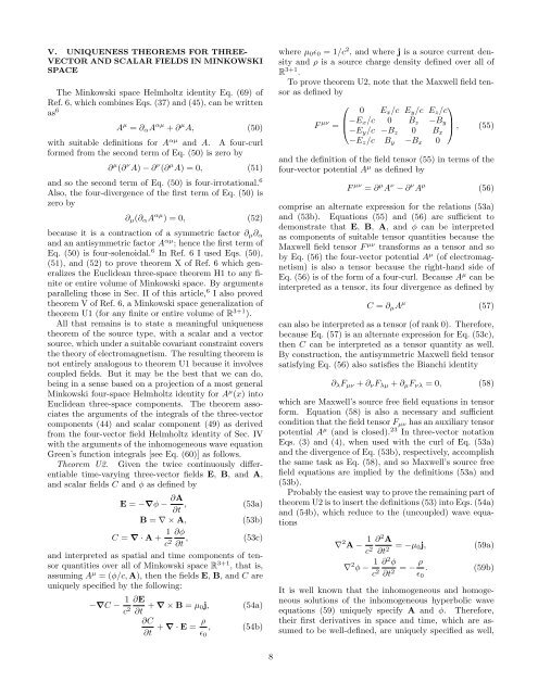
V. UNIQUENESS THEOREMS FOR THREE-VECTOR AND SCALAR FIELDS IN MINKOWSKISPACEThe Minkowski space Helmholtz identity Eq. (69) ofRef. 6, which combines Eqs. (37) and (45), can be writtenas 6 A µ = ∂ α A αµ + ∂ µ A, (50)with suitable definitions for A αµ and A. A four-curlformed from the second term of Eq. (50) is zero by∂ µ (∂ ν A) − ∂ ν (∂ µ A) = 0, (51)and so the second term of Eq. (50) is four-irrotational. 6Also, the four-divergence of the first term of Eq. (50) iszero by∂ µ (∂ α A αµ ) = 0, (52)because it is a contraction of a symmetric factor ∂ µ ∂ αand an antisymmetric factor A αµ ; hence the first term ofEq. (50) is four-solenoidal. 6 In Ref. 6 I used Eqs. (50),(51), and (52) to prove theorem X of Ref. 6 which generalizesthe Euclidean three-space theorem H1 to any finiteor entire volume of Minkowski space. By argumentsparalleling those in Sec. II of this article, 6 I also provedtheorem V of Ref. 6, a Minkowski space generalization oftheorem U1 (for any finite or entire volume of R 3+1 ).All that remains is to state a meaningful uniquenesstheorem of the source type, with a scalar and a vectorsource, which under a suitable covariant constraint coversthe theory of electromagnetism. The resulting theorem isnot entirely analogous to theorem U1 because it involvescoupled fields. But it may be the best that we can do,being in a sense based on a projection of a most generalMinkowski four-space Helmholtz identity for A µ (x) intoEuclidean three-space components. The theorem associatesthe arguments of the integrals of the three-vectorcomponents (44) and scalar component (49) as derivedfrom the four-vector field Helmholtz identity of Sec. IVwith the arguments of the inhomogeneous wave equationGreen’s function integrals [see Eq. (60)] as follows.Theorem U2. Given the twice continuously differentiabletime-varying three-vector fields E, B, and A,and scalar fields C and φ as defined byE = −∇φ − ∂A∂t ,(53a)B = ∇ × A,(53b)C = ∇ · A + 1 ∂φc 2 ∂t ,(53c)and interpreted as spatial and time components of tensorquantities over all of Minkowski space R 3+1 , that is,assuming A µ = (φ/c, A), then the fields E, B, and C areuniquely specified by the following:−∇C − 1 ∂Ec 2 ∂t + ∇ × B = µ 0j,∂C∂t + ∇ · E = ρ ,ɛ 0(54a)(54b)where µ 0 ɛ 0 = 1/c 2 , and where j is a source current densityand ρ is a source charge density defined over all ofR 3+1 .To prove theorem U2, note that the Maxwell field tensoras defined by⎛⎞0 E x /c E y /c E z /cF µν ⎜−E = x /c 0 B z −B y ⎟⎝−E y /c −B z 0 B⎠ , (55)x−E z /c B y −B x 0and the definition of the field tensor (55) in terms of thefour-vector potential A µ as defined byF µν = ∂ µ A ν − ∂ ν A µ (56)comprise an alternate expression for the relations (53a)and (53b). Equations (55) and (56) are sufficient todemonstrate that E, B, A, and φ can be interpretedas components of suitable tensor quantities because theMaxwell field tensor F µν transforms as a tensor and soby Eq. (56) the four-vector potential A µ (of electromagnetism)is also a tensor because the right-hand side ofEq. (56) is of the form of a four-curl. Because A µ can beinterpreted as a tensor, its four divergence as defined byC = ∂ µ A µ (57)can also be interpreted as a tensor (of rank 0). Therefore,because Eq. (57) is an alternate expression for Eq. (53c),then C can be interpreted as a tensor quantity as well.By construction, the antisymmetric Maxwell field tensorsatisfying Eq. (56) also satisfies the Bianchi identity∂ λ F µν + ∂ ν F λµ + ∂ µ F νλ = 0, (58)which are Maxwell’s source free field equations in tensorform. Equation (58) is also a necessary and sufficientcondition that the field tensor F µν has an auxiliary tensorpotential A µ (and is closed). 23 In three-vector notationEqs. (3) and (4), when used with the curl of Eq. (53a)and the divergence of Eq. (53b), respectively, accomplishthe same task as Eq. (58), and so Maxwell’s source freefield equations are implied by the definitions (53a) and(53b).Probably the easiest way to prove the remaining part oftheorem U2 is to insert the definitions (53) into Eqs. (54a)and (54b), which reduce to the (uncoupled) wave equations∇ 2 A − 1 c 2 ∂ 2 A∂t 2 = −µ 0j, (59a)∇ 2 φ − 1 c 2 ∂ 2 φ∂t 2 = − ρ ɛ 0. (59b)It is well known that the inhomogeneous and homogeneoussolutions of the inhomogeneous hyperbolic waveequations (59) uniquely specify A and φ. Therefore,their first derivatives in space and time, which are assumedto be well-defined, are uniquely specified as well,8
and so by the definitions (53) the fields E, B, and C areuniquely specified and theorem U2 is proved. Note that ifEq. (54a) is substituted into identity (44), and Eq. (54b)is substituted into identity (49), we obtain∫A(x) = µ 0 j(x ′ )G(x, x ′ )d 4 x ′ , (60a)φ(x)c= 1 cV 4′∫V ′4ρ(x ′ )ɛ 0G(x, x ′ )d 4 x ′ , (60b)which are inhomogeneous solutions of the wave equations(59) in terms of a suitable Green’s function. It was theGreen’s function solution of Eq. (17b) which led via thedelta function identity (23a) to the spatial components(37) and time component (45) of the A µ identity itself. 6Equations (54a) and (54b) reduce to Maxwell’s sourceequations if we set the four-divergence C = ∂ µ A µ = 0,that is, with the Lorentz gauge condition (more descriptivelycalled a relativistic transverse gauge condition). 6,7It is easily proved that once this relativistic transversegauge condition is assumed, the resulting Maxwell’sequations decouple to give the wave equations (59). Themost general Lagrangian density for a (massless) fourvectorfield A µ that is no more than quadratic in its variablesand their derivatives, 6 and which embodies theoremU2 via the covariant formalism (55)−(57), appears to beL = − ɛ 0c 24 F µνF µν − λɛ 0c 22(∂ µ A µ ) 2 + j µ A µ , (61)where j µ = (ρc, j) and λ is a Lagrange multiplier for theLorentz constraint term. The covariant Lagrange equationof motion which follows from Eq. (61) is−j ν /ɛ 0 c 2 = ∂ µ F µν + λ∂ ν (∂ µ A µ )(62a)= ∂ µ ∂ µ A ν − (1 − λ)∂ ν (∂ µ A µ ). (62b)If we make the physical assumption that all derivatives∂ µ have equal weight, we may set λ = 1, which reducesEq. (62b) to□A ν = ∂ µ ∂ µ A ν = −j ν /ɛ 0 c 2 = −µ 0 j ν , (63)which is the wave equations (59) in covariant notation.There is another covariant gauge that I have dubbedthe relativistic longitudinal gauge, 6,7 where the four-curlF µν = 0, which implies via Eq. (55) that E = 0 andB = 0 as well. With this relativistic longitudinal gaugecondition the Lagrange equation of motion (62b) reduces(with λ = 1) to−j ν /ɛ 0 c 2 = ∂ ν (∂ µ A µ ) = ∂ µ (∂ ν A µ ) = ∂ µ (∂ µ A ν ), (64)where ∂ µ A ν = ∂ ν A µ in this gauge via Eq. (56), which isalso the wave equations (59) in covariant notation. Similarly,in three-vector notation the field equations (54)and definitions (53) of theorem U2 for the relativisticlongitudinal gauge condition reduce to−∇(∇ · A) − 1 ∂(∇φ)c 2 = −∇C = µ 0 j,∂t(65a)∇ · ∂A∂t + 1 ∂ 2 φc 2 ∂t 2 = ∂C∂t = ρ .ɛ 0(65b)The relativistic longitudinal gauge condition F µν = 0implies thatE = −∇φ − ∂A∂t = 0,B = ∇ × A = 0,(66a)(66b)so that, with the identity (8), it follows that Eqs. (65a)and (65b) reduce to the wave equations (59).VI.CONCLUDING REMARKSIt can be argued that theorem U2 uniquely specifiesthe most general three-vector and scalar field (component)equations in Minkowski space for an associated(massless) classical four-vector field A µ that is assumedto satisfy an inhomogeneous hyperbolic wave equation.That is, the field definitions and equations of theoremU2 follow directly from the use of a Green’s functionsolution technique using an operator delta function fourvectoridentity. Thus, it should not be surprising thatboth the relativistic transverse and relativistic longitudinalcovariant gauge conditions, when used in conjunctionwith theorem U2, lead to the same wave equations. Ihave previously shown that the relativistic transverse andrelativistic longitudinal covariant gauge conditions leadrespectively to only two classes of classical four-vectorfields which are potentially physical. 7 By the latter it ismeant that a suitable fully quadratic Lagrangian density(of the type used here but more general in that it has afield mass term and can have complex valued charges) isbounded from below when one or the other of these twocovariant gauge conditions is applied. 7ACKNOWLEDGMENTSThe author thanks Andrew Stewart of the ResearchSchool of Physical Sciences and Engineering at The AustralianNational University for prompting the author toinvestigate the uniqueness of time-varying three-vectorfields in relation to his work in Ref. 17, and for subsequentreview of this paper. The author also thanks J. V.Corbett of the Department of Mathematics of MacquarieUniversity−Sydney for detailed review of this paper. Theauthor is indebted to James Cresser of the Departmentof Physics of Macquarie University−Sydney for supportof the author’s research position in the department.9
Page 2 and 3: Theorem U1. The divergence and curl
Page 4 and 5: volume and its associated finite vo
Page 6 and 7: set the divergence of Eq. (29) equa
Page 10: a) Electronic mail: dalew@ics.mq.ed

Three-vector and scalar field identities and uniqueness theorems in ...

You also want an ePaper? Increase the reach of your titles

Delete template?

Save as template?