Three-vector and scalar field identities and uniqueness theorems in ...

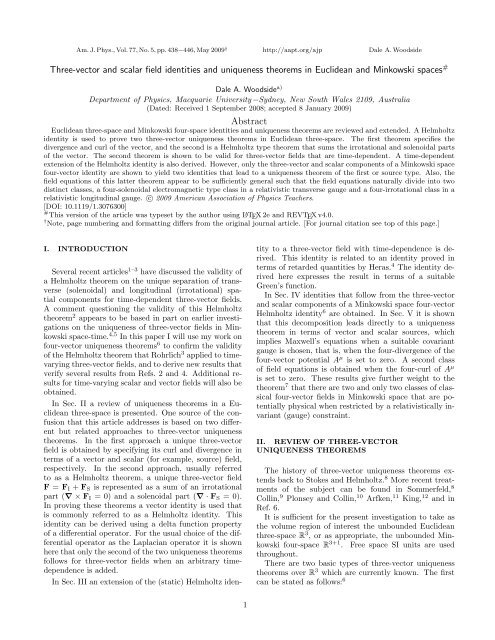
Theorem U1. The divergence and curl of a twice continuouslydifferentiable (static) three-vector field, whichvanishes sufficiently rapidly at infinity, uniquely determinesthe three-vector field over an unbounded volumeV of R 3 .In other words, we must specify∇ × F(x, y, z) = j(x, y, z),∇ · F(x, y, z) = ρ(x, y, z),(1a)(1b)over the volume V. In an electromagnetic context j isa circulation current density and ρ is a source chargedensity. A proof of a version of this theorem over a finitevolume of R 3 is given in Ref. 11.The second uniqueness theorem, which is typicallycalled a Helmholtz theorem, can be stated as follows: 6Theorem H1. A general continuous three-vector fielddefined everywhere in R 3 that along with its first derivativesvanishes sufficiently rapidly at infinity may beuniquely represented as a sum of an irrotational and asolenoidal part, up to a possible additive constant vector.A proof of theorem H1 is given in Ref. 8. To prove thistheorem it is sufficient to prove only that the three-vectorF can be written as 11F(x, y, z) = −∇Φ(x, y, z) + ∇ × A(x, y, z). (2)Then the three-vector identity∇ × ∇Φ = 0, (3)and the irrotational field assumption ∇ × F I = 0 impliesthat F I = −∇Φ is irrotational. And the three-vectoridentity∇ · ∇ × A = 0, (4)and the solenoidal field assumption ∇ · F S = 0 impliesthat F S = ∇ × A is solenoidal. Thus Eq. (2) is a sum ofan irrotational and a solenoidal part.The most straightforward proof of Eq. (2) (see Refs. 9and 10) and therefore of theorem H1 is to obtain a Helmholtzidentity 8 that is of the same form as Eq. (2). Aproof of this identity is presented here so that our analysisis self contained. This proof is based on the assumptionthat there exists a solution for a three-vectorF of an inhomogeneous vector Poisson equation in Cartesiancoordinates, and that each separate Cartesian componentof F is a solution of a scalar Poisson equation.The scalar Poisson equation can then be solved in termsof a two-point scalar Green’s function G(r, r ′ ) that connectsits unit delta function source located at the sourcepoint r ′ = (x ′ , y ′ , z ′ ) to a measurement at the field pointr = (x, y, z). Because∇ 2 14πr = −δ3 (r − r ′ ), (5)for all r and r ′ with r ≡ |r − r ′ |, the Poisson equationdefining the Green’s function,∇ 2 G(r, r ′ ) = −δ 3 (r − r ′ ), (6)leads to G(r, r ′ ) = 1/4πr. The delta function property ofthe vector identity (5) can be applied to any well-behavedfunction F(x, y, z) as∫F(x, y, z) = F(x ′ , y ′ , z ′ )δ 3 (r − r ′ )dV ′ (7a)V∫′ ( ) −1= F(x ′ , y ′ , z ′ )∇ 2 dV ′ . (7b)V 4πr′Because the Laplacian operator acts only on the fieldpoint coordinates, it can be brought outside of the integrationover the source point coordinates. We can usethe well known three-space identity∇ 2 A = ∇(∇ · A) − ∇ × (∇ × A) (8)to rewrite Eq. (7b) as [typo corrected from journal article]∫F(x, y, z) = − ∇ ∇ · F(x′ , y ′ , z ′ )dV ′V 4πr′∫+ ∇ × ∇ × F(x′ , y ′ , z ′ )dV ′ , (9)V 4πr′where one of the ∇ operators has been brought backinto each of the integrals, which is allowed because theyoperate only on the field coordinates. Although Eq. (9)is in a form like Eq. (2) as required to prove theorem H1,it is necessary to obtain an identity that is suitable toprove the three-space theorem U1 as well. If we use thevector identities 10∇ · (φA) = A · ∇φ + φ∇ · A,∇ × (φA) = −A × ∇φ + φ∇ × A,(10a)(10b)(note that the divergence and curl equal zero with respectto the field coordinates of a vector A which is a functiononly of the source coordinates) and use the identity∇(1/r) = −∇ ′ (1/r), we find∫F(x, y, z) = ∇ F(x ′ , y ′ , z ′ ) · ∇ ′ 1V 4πr dV ′′∫+∇ ×V ′ F(x ′ , y ′ , z ′ ) × ∇ ′ 14πr dV ′ . (11)The vector identities (10) are now applied again, this timeon the integrands of Eq. (11) where the ∇ operators acton the source coordinates. We obtain four terms; the onescontaining ∇ · (φA) and ∇ × (φA), respectively, becomesurface integrals via the following identities, 10 (that is,letting T = φA),∫∮ ∮∇ · T dV = T · dS = T · n dS, (12a)VSS∫∮∮∇ × T dV = n × T dS = − T × n dS, (12b)VSwhere n is the unit surface normal of S bounding V .These integrals vanish as r → ∞ for the field F, whichis assumed to fall off sufficiently rapidly at infinity. TheS2

final two terms are now of the proper form yielding thedesired identity∫∇ ′ · F(x ′ , y ′ , z ′ )F(x, y, z) = − ∇dV ′V 4πr∫′ ∇ ′ × F(x ′ , y ′ , z ′ )+ ∇ ×dV ′ (13)V 4πr′over all Euclidean three-space.A proof of Eq. (13) can be traced back to Stokes. 8 Nevertheless,Eq. (13) is sometimes referred to as a “Helmholtzidentity” (see Ref. 10). For an extended versionof Eq. (13) in a finite volume of R 3 the surface integralterms can be retained. 6,9,10 Equation (13) is of the formof Eq. (2) and can therefore be considered as completingthe proof of theorem H1, provided that the integrals arewell defined. For the integrals to be well defined we mustassume that the field F vanishes sufficiently rapidly atinfinity. As noted in Ref. 6, passing the remaining vectorderivatives over the field point coordinates for a twicecontinuously differentiable vector field F into each of therespective integrals of Eq. (13) can improve the convergenceproperties of the integrands.To prove theorem U1 using the Helmholtz identity (13)for the (static) three-vector field F(r) we postulate theexistence of a second three-vector field G(r), which alsosatisfies Eqs. (1) and (13). That is, we replace F(r) onthe left-hand side of Eqs. (1a) and (1b) by G(r), leavingthe right-hand side of Eqs. (1a) and (1b) unchanged. Thethree-vector field F(r) is unique if we can show thatW(r) ≡ F(r) − G(r) = 0. (14)If we take the divergence of W and use Eq. (1b), weobtain∇ · W = ∇ · F − ∇ · G = ρ − ρ = 0 (15)for all r in R 3 . We next take the curl of W and useEq. (1a) to obtain∇ × W = ∇ × F − ∇ × G = j − j = 0 (16)for all r in R 3 . The substitution of the results (15) and(16) for the three-vector field W into the Helmholtz identity(13) yields the result W(r) = 0 which implies [viathe definition of W(r) in Eq. (14)] that F(r) = G(r)everywhere in R 3 . This proof implies that the (static)three-vector field F is uniquely determined by Eqs. (1a)and (1b), thus proving theorem U1 on the uniqueness of(static) three-vector fields in terms of their curl and divergence,that is, in terms of a vector and a scalar (source)field, respectively. [For a finite volume of R 3 the normalcomponents W·n and tangential components W×n alsovanish in a similar fashion via a surface charge density σand surface current density K, as can be shown for examplein an explicit calculation for the case of a massive(static) three-vector field. 6 ]We now state the obvious. Equations (1a) and (1b) associatedwith theorem U1 are not equivalent to Maxwell’sequations, which uniquely specify the electromagneticfields. They do not contain any partial time derivativeterms and do not contain any coupling between differentthree-vector fields. Therefore, Eqs. (1a) and (1b)and theorem U1 do not hold for time-varying electricand magnetic fields, which are examples of hyperbolicallypropagating 4 time-varying three-vector fields. Therefore,theorem U1 does not hold for all time-varying threevectorfields because there is at least one counterexample,that is, electromagnetism.In contrast, the Helmholtz theorem H1 is quite differentin scope. It is essentially a projection theorem whichuses three-vector analysis to project out the longitudinal(irrotational) parts (which have zero curl) and transverse(solenoidal) parts (which have zero divergence) ofan arbitrary three-vector field, and states that any threevectorfield can be represented as a sum of these twoparts. To show that this theorem holds even for timedependentthree-vectors, it is sufficient to verify the stepsemployed in deriving the Helmholtz identity (13), becauseit is of the proper form of Eq. (2), which is sufficientto prove theorem H1. Following this line of reasoning,first observe that the delta function integral propertyin Eq. (7b) holds even for well-behaved time-varyingthree-vector functions F(x, y, z, t) because the space andtime variables are independent, and consequently spaceand time integrations are performed separately. As forEq. (8), it is a three-vector identity over the Euclideanvector space R 3 and over the associated scalars in thereal number field R which applies to any (even timedependent)three-vector because it is based on multiplicationof vectors by scalars (a defining property of a vectorspace) and on the two principal ways that vectors canbe multiplied by each other in R 3 , that is, dot and crossproducts. [More formally, for A as a time-dependentvariable, Eq. (8) forms a one parameter family of vectorfields parametrized by t. For each time t, Eq. (8) holds.The same can be said for Eq. (7b).] Equation (8) is oftenused in deriving the spatial parts of wave equations andis the principal vector identity that leads to the decomposition(2). For the same reasons the vector identities(10) and integral identities (12) are valid for time-varyingfields. Therefore, the Helmholtz identity (13) holds evenfor time-varying three-vector fields and so Helmholtz’stheorem H1 follows for them as well via Eq. (2).Helmholtz’s theorem H1 has been used frequently withtime-varying fields in both classical and quantum mechanicalcontexts. Rohrlich 3 has demonstrated that thisHelmholtz decomposition holds even for electromagneticsources, provided that the sources are bounded in space.This latter requirement is essentially equivalent to thecase of the general fields discussed here which are assumedto vanish sufficiently rapidly at infinity in unboundedR 3 . The relevant requirement in a bounded volumeV of R 3 is that the vector (or scalar) field must besufficiently smooth, 6 that is, a twice continuously differentiablefunction on the union of V and its boundingsurface S, in order that a Helmholtz identity in a finite3

volume and its associated finite volume Helmholtz theoremis satisfied. 6,9,10 Equation (13) has also been used ina time-varying context to demonstrate its compatibilitywith electromagnetism in the Coulomb gauge, and to derivethe Aharonov-Bohm transverse vector potential. 13–16The Helmholtz theorem was recently used to prove a vectoridentity for the volume integral of the square of avector field which could be time-varying, and Eq. (13)was used to derive two expressions for the energy of theelectromagnetic field. 17III. A TIME-DEPENDENT HELMHOLTZIDENTITYA logical next step for a three-vector field that is requiredto propagate via an inhomogeneous hyperbolicwave equation in terms of its three-vector (current)source is to derive an extension of the three-vector Helmholtzidentity by choosing the d’Alembertian wave equationoperator as the differential operator used to obtainan associated delta function identity. If we assume Cartesiancoordinates, it is sufficient to solve an inhomogeneousscalar d’Alembertian wave equation in terms of atwo-point scalar Green’s function G(x ν , x ′ν ) which connectsits unit delta function source located at the spacetimesource point x ′ν to a measurement at the space-timefield point x ν = (ct, x, y, z) in R 3+1 . That is,□G(x ν , x ′ν ) =(∇ 2 − 1 ∂ 2 )c 2 ∂t 2 G(x ν , x ′ν ) (17a)= −δ(x 0 − x ′0 )δ 3 (r − r ′ ) = −δ (4) (x ν − x ′ν ). (17b)An example of a Green’s function that satisfies Eq. (17b)assuming timelike causality is the familiar retardedGreen’s function as derived for example by Cushing 18or Jackson, 19 which for the metric signature (− + ++)used in this article isG ret (r, r ′ ; t, t ′ ) = 14πδ(|r − r ′ | − c(t − t ′ ))|r − r ′ , (18)|for t > t ′ . The retarded Green’s function (18) is derivedvia a spectral decomposition of the delta function,taking into account homogeneous boundary conditionson a closed spatial surface, as well as timelikecausality with the initial conditions G(r, r ′ ; t, t ′ ) = 0 and∂G(r, r ′ ; t, t ′ )/∂t = 0 for t < t ′ , and the Green’s functionsymmetry relationG(r, r ′ ; t, t ′ ) = G(r ′ , r; −t ′ , −t). (19)For a relativistically invariant version of Eq. (18), thatis, G ret (x, x ′ ), and for the advanced Green’s functionG adv (x, x ′ ), see for example Ref. 6. (In what followsthe usual shorthand notation is adopted, and the superscriptsin the functional dependencies are droppedfor brevity.) The spectral decomposition of the fourspacedelta function of Eq. (17b) also yields certain requiredcovariant and contravariant derivative propertiesof G(x, x ′ ) in Minkowski space: 6∂ µ G(x, x ′ ) = − ∂ ′ µG(x, x ′ ),∂ µ G(x, x ′ ) = − ∂ ′µ G(x, x ′ ).(20a)(20b)With ∂ µ = ((1/c)∂/∂t, ∇) and ∂ µ = (−(1/c)∂/∂t, ∇) weobtain the space and time components of Eq. (20a) as∂ i G(x, x ′ ) = − ∂ iG(x, ′ x ′ ),∂ 0 G(x, x ′ ) = − ∂ 0G(x, ′ x ′ ),(21a)(21b)with equivalent relations for the contravariant derivatives.Note that Eq. (21a) is analogous to the relation∇(1/r) = −∇ ′ (1/r) used in R 3 which can be rewrittenas ∇G(r, r ′ ) = −∇ ′ G(r, r ′ ). In R 3+1 there is the additionaltime derivative property (21b). For the presentanalysis Eqs. (21a) and (21b) can be written simply as∇G(x, x ′ ) = −∇ ′ G(x, x ′ ),(22a)∂G(x, x ′ )= − ∂G(x, x′ )∂t∂t ′ . (22b)The delta function property (17b) can be applied forany well-behaved function F(x ν ) as an integration overthe unbounded four-volume V 4 ′ of R 3+1 as follows:∫F(x) = F(x ′ )δ (4) (x − x ′ ) d 4 x ′(23a)∫=V 4′V ′4F(x ′ )□(−G(x, x ′ )) dV ′ c dt ′ .(23b)It is not necessary at this point to specify the choiceof a particular Green’s function G(x, x ′ ), other thanthat it satisfies Eq. (17b). In fact, there is a distinctadvantage to not choosing a retarded (advanced)Green’s function for doing the time integration at thispoint because the resulting retarded (advanced) threevectorfields are much more difficult with which to work.In contradistinction, the space and time derivatives ofa three-vector with unmixed arguments, for example,F(x ′ ) = F(ct ′ , x ′ , y ′ , z ′ ), needs no special treatment.Consequently, the entire (spatial) derivation of the Helmholtzidentity (13), in view of the equivalent form of relation(22a), can be used with Eq. (23b), yielding∫F(x) = −∇ ∇ ′ · F(x ′ )G(x, x ′ ) dV ′ c dt ′V 4′∫+ ∇ ×+ 1 c 2 ∂∂tV 4′∫V ′4∇ ′ × F(x ′ )G(x, x ′ ) dV ′ c dt ′∂(F(x ′ )G(x, x ′ ))∂tdV ′ c dt ′ , (24)where one of the unprimed partial time derivatives hasbeen taken outside of the integration over the primedtime derivative, and the other has been put in front ofF(x ′ ). The application of the time derivative in the integrandof the third term of Eq. (24) gives∂(F(x ′ )G(x, x ′ ))∂t= −F(x ′ ) ∂G(x, x′ )∂t ′(25a)= − ∂(F(x′ )G(x, x ′ ))∂t ′ + ∂F(x′ )∂t ′ G(x, x ′ ), (25b)4

where the unprimed time derivative of F(x ′ ) is zero and where a minus sign has been introduced in the substitutionsE(ct, x, y, z) = −∇φ − ∇ × K − ∂A∂t , (29) be adequate to generate a new uniqueness theorem of thetype of theorem U1. To demonstrate this deficiency weEq. (22b) has been used in Eq. (25a). The time integrationfor the second and third terms of Eq. (29) to empha-of the first term of Eq. (25b) can be assumed tovanish as t ′ → ±∞ for the field F which is assumed tobe bounded in time. Therefore, only the second term ofEq. (25b) contributes to Eq. (24), reducing it tosize its similarity to a well-known definition of the electricfield in terms of the electric and magnetic potentials. 20A compatible definition of the magnetic field 20 with appropriatevariable and sign changes would be∫F(x) = −∇ ∇ ′ · F(x ′ )G(x, x ′ ) dV ′ c dt ′B(ct, x, y, z) = −∇ξ + ∇ × A − ∂K∂t . (30)V 4∫′+ ∇ × ∇ ′ × F(x ′ )G(x, x ′ ) dV ′ c dt ′ In a different calculation on a related subject, Eq. (13) inRef. 4 [similar to Eq. (28) here] was used to derive an extensionof Jefimenko’s time-dependent generalizations ofV 4′+ 1 ∫∂ ∂F(x ′ )c 2 ∂t V 4′ ∂t ′ G(x, x ′ ) dV ′ c dt ′ , (26) the Coulomb and Biot-Savart laws 21 to include magneticcharge and current sources. The time-dependent Helmholtzidentity (26) therefore has interesting applications.which can be regarded as a time-dependent generalizationof the (static) Helmholtz identity (13) for any tion of Eq. (2) via the time-dependent Helmholtz iden-Although Eq. (29) is an example of the generaliza-suitable Green’s function G(x, x ′ ) that is a solution of tity (26), it is the possibility of using Eq. (26) to obtainEq. (17b). [A result like Eq. (26), but in terms of a retardedGreen’s function, was given in Ref. 2 with a com-the claim by Heras 2 that the terms of Eq. (26) could beuniqueness theorems that is of interest here. Considerment that the proof followed from Eq. (23b); we have labeled (preserving the order of the terms) as follows:verified this proof in detail here.] If we substitute theretarded Green’s function (18) into Eq. (26) we obtainE(ct, x, y, z) = E ‖ + E ⊥ + E T . (31)∫F(x) = −∇ ∇ ′ · F(x ′ ) δ(r − c(t − t′ ))dV ′ c dt ′ The longitudinal component E ‖ is irrotational and satisfiesV 4′4πr∫+ ∇ × ∇ ′ × F(x ′ ) δ(r − c(t − t′ ))dV ′ c dt ′∇ × E ‖ = 0, (32)V 4′4πr+ 1 ∫∂ ∂F(x ′ ) δ(r − c(t − t ′ and the transverse component E))⊥ is solenoidal and satisfiesc 2 ∂t V 4′ ∂t ′ dV ′ c dt ′ .4πr(27)∇ · E ⊥ = 0. (33)When the time integration in Eq. (27) is performed,the argument of the delta function implies that all t ′dependent variables in the integrand are evaluated att − r/c. If we use a retarded potential bracket notationThe time component E T may have both transverse andlongitudinal components. The first term of Eq. (26) is alongitudinal component via Eq. (3) and the second termof Eq. (26) is a transverse component via Eq. (4). However,Heras 4 states in this context that “the specificationwhere [P(r ′ , ct ′ )] ret denotes evaluation at the retardedtime t ′ = t − r/c, then Eq. (27) can be rewritten as of ∂F/∂t is not available in general and there is not asimple approach for obtaining it.”∫[∇ ′ · F(r ′ , ct ′ )] retThe salient issue here is that the divergence and curlF(x) = −c∇dV ′V 4πroperations are sufficient to produce all the possible projectionsof vector fields in R 3 . That is, the application of∫′[∇ ′ × F(r ′ , ct ′ )] ret+ c∇ ×dV ′a time partial derivative cannot project out a time componentlongitudinal to the time dimension from a three-V 4πr′+ 1 ∫ [∂ ∂F(r ′ , ct ′ ) 1c ∂t V ∂t]ret′ 4πr dV ′ vector field that has only spatial dimensions. Four-vector, (28)fields are required for that. All that has been done here′is that an independent (time) variable has been included,which is similar to Eq. (13) in Ref. 4. The result (28) isobtained here in a more easily verified manner becausewithout forming a vector space of one more dimension.The absence of a unique specification of a time projectiontricky retarded potential calculations are avoided by retainingfor the hypothetical time component E T belonging tothe general Green’s function G(x, x ′ ) through tothe time-dependent Helmholtz identity (26).the three-vector space R 3 makes it problematic for thereto be a time-dependent version of theorem H1 based onWith suitable substitutions the identity (26) can be Eq. (31) [or Eq. (26)].rewritten in a form resembling Eq. (2) asNeither does Eq. (29), as a representative example ofa choice of variables following from Eq. (26), appear to5

set the divergence of Eq. (29) equal to a suitable (electric)scalar source charge density ρ e scaled by the free spacepermittivity constant ɛ 0 yieldingρ e= ∇ · E = −∇ · ∇φ − ∂∇ · A , (34)ɛ 0 ∂twhere the second term of Eq. (29) vanishes via Eq. (4).Then we set the curl of Eq. (29) equal to a suitable (magnetic)three-vector current density j m scaled by the freespace permeability constant µ 0 yielding−µ 0 j m = ∇ × E = −∇ × ∇ × K − ∂∇ × A , (35)∂twhere the first term of Eq. (29) vanishes via Eq. (3).Then we take the partial time derivative of Eq. (29) yielding∂E∂t = −∇∂φ ∂t − ∂∇ × K − ∂2 A∂t ∂t 2 . (36)In contrast to Eqs. (34) and (35) it is not evident whatsource density should be equated to the left-hand side ofEq. (36). In the present context of a time-varying electromagnetismwith both electric and magnetic charges, sucha third source relation would be inconsistent because theremaining two sources, ρ m and j e , would need to be accountedfor by the compatible relation (30). In addition,although Eq. (34) is adequate for the time-varying case,Eq. (35) is adequate only for static fields [compare withEq. (11) in Ref. 4]. If there are no magnetic sources,j m , ρ m , ξ, and K vanish and then Eq. (35) also lacks asource to uniquely specify it (or is reduced to no morethan the static case by setting j m = 0). Equation (30)suffers from similar difficulties with relations analogousto Eqs. (35) and (36). Consequently, it is problematicfor there to be a time-dependent version of theorem U1based on Eqs. (29) and (30) [or Eq. (26)] for the mostgeneral electromagnetic case.IV. TIME-DEPENDENT THREE-VECTORAND SCALAR FIELD IDENTITIESIn Sec. III it was shown that the use of the timedependentgeneralization (26) of the (static) Helmholtzidentity (13) does not appear to be adequate to obtaintime-dependent versions of uniqueness theorems U1 orH1. However, an “extended curl” 5 approach for obtaininga uniqueness theorem for a pair of coupled timedependentthree-vector fields in terms of two scalar andtwo three-vector source fields, and in terms of two auxiliaryfield definitions such as Eqs. (29) and (30), wasformulated in Ref. 22. This latter theorem was referredto there as a generalized Helmholtz theorem. 22 From ourpoint of view the first part of this two part theorem is oftype U1, and the second part is of the Helmholtz (projection)type H1, although the concepts of irrotationaland solenoidal are omitted. The proof is based on theexistence of nontrivial solutions of the associated ellipticalor hyperbolic differential equations. In the hyperboliccase the field equations can be used to treat the electromagneticcase with both electric and magnetic charges.As interesting as this theorem is, its equations are notderived from first principles, but are postulated in theirentirety. Secondly, it is a theorem for three-vectors in R 3with the time-dependence put in by hand, that is, it is notmanifestly covariant. It will be shown here that a manifestlycovariant approach 6 in R 3+1 can yield the desiredtime-varying uniqueness theorems that do not appear tofollow from first principles in R 3 .It has been previously shown (by taking a static Newtonianlimit) that the spatial components of the identityEq. (69) of theorem II of Ref. 6 [see Eq. (37)] is a Minkowskispace generalization of the (Euclidean three-space)Helmholtz identity (13), but more generally in a finitevolume of R 3 . In addition, the fourth or scalar field componentof this identity [see (Eq. 45)] was shown to yield ascalar field identity, Eq. (96) of Ref. 6, in a similar staticNewtonian limit. To obtain the full time-dependent resultswe first take the space components of this identity(that is, where the four-space index µ is replaced by thethree-space index j):[ ∫A j (x) = −∂ j ∂ νA ′ ν (x ′ )G(x, x ′ )d 4 x ′V 4′](A∮Σ ν (x ′ )n ′ ν)G(x, x ′ )dΣ ′′−[ ∫− ∂ α (∂ ′α A j (x ′ ) − ∂ ′j A α (x ′ ))G(x, x ′ )d 4 x ′V 4′]+ (A∮Σ α (x ′ )n ′j − A j (x ′ )n ′α )G(x, x ′ )dΣ ′ , (37)′where the four-volume region V 4 ′ of Minkowski space-timeis bounded by the three-surface Σ ′ , and the unprimedderivatives have been factored out of the primed coordinateintegrals. If we adopt three-vector notation andallow the four-volume region V 4 ′ to expand to includeall Minkowski space-time so that the three-surface integralscan be dropped [under the assumption that thefour-vector field A µ (x) = (φ/c, A) vanishes sufficientlyrapidly at infinity], we can simplify Eq. (37) to∫A(x) = −∇− 1 ∫∂c ∂t∫+ ∇ ×V 4′V 4′V ′4(∇ ′ · A(x ′ ) + 1 ∂φ(x ′ ))c 2 ∂t ′(− 1 ∂A(x ′ )c ∂t ′ − ∇′ φ(x ′ )cG(x, x ′ )d 4 x ′)G(x, x ′ )d 4 x ′(∇ ′ × A(x ′ ))G(x, x ′ )d 4 x ′ , (38)where the first four-volume integral of Eq. (38) followsfrom the first four-volume integral of Eq. (37), the secondfour-volume integral of Eq. (38) follows from the α = 06

component of the second four-volume integral of Eq. (37),and the third four-volume integral of Eq. (38) followsfrom that same term’s α = i spatial components by comparingthe implied sum on i for each of the j = 1, 2, 3components with the components of the vector triplecross product in Eq. (38). If we make the change of variables[using the components of the four-curl of A µ , thatis, Maxwell’s field tensor F µν , see Eqs. (55) and (56)]withE = −∇φ − ∂A , B = ∇ × A, (39)∂tand the change of variables [using the four-divergence ofA µ , see Eq. (57)] withwe can reduce Eq. (38) to∫A(x) = − ∇C = ∇ · A + 1 c 2 ∂φ∂t , (40)V 4′− 1 ∫∂c 2 ∂t∫+ ∇ ×C(x ′ )G(x, x ′ )d 4 x ′V ′4V ′4E(x ′ )G(x, x ′ )d 4 x ′B(x ′ )G(x, x ′ )d 4 x ′ . (41)We can move the unprimed ∇ operator into the first(primed) integral of Eq. (41), and then as for Eq. (25),we can express the argument of the integral as∇(C(x ′ )G(x, x ′ )) = −C(x ′ )∇ ′ G(x, x ′ )(42a)= −∇ ′ (C(x ′ )G(x, x ′ )) + (∇ ′ C(x ′ ))G(x, x ′ ), (42b)because the unprimed gradient of C(x ′ ) is zero and theGreen’s function property (22a) is used in Eq. (42a).Note that∫V ′ ∇ ′ (C(x ′ )G(x, x ′ ))dV ′ = 0 (43)over the infinite three-volume V ′ for the scalar fieldC(x ′ ), which is assumed to vanish sufficiently rapidlyat infinity because A and φ are assumed to do so also.Therefore, only the second term of Eq. (42b) contributesto Eq. (41). If we use the result (25b) on the second integralof Eq. (41), assume that E is bounded in time, anduse Eq. (10b) and the surface integral argument that ledto Eq. (13) on the third integral of Eq. (41), we obtainthe desired three-vector field identity∫A(x) =V ′4(−∇ ′ C(x ′ ) − 1 ∂E(x ′ )c 2 ∂t ′)+ ∇ ′ × B(x ′ ) G(x, x ′ )d 4 x ′ . (44)In a similar fashion a scalar component of the identityEq. (69) of Ref. 6 can be obtained as follows:[ ∫A 0 (x) = − ∂ 0 ∂ νA ′ ν (x ′ )G(x, x ′ )d 4 x ′V 4′](A∮Σ ν (x ′ )n ′ ν)G(x, x ′ )dΣ ′′−[ ∫(− ∂ α ∂ ′α A 0 (x ′ ) − ∂ ′ 0 A α (x ′ ) ) G(x, x ′ )d 4 x ′V 4′]+ (A∮Σ α (x ′ )n ′ 0 − A 0 (x ′ )n ′α )G(x, x ′ )dΣ ′ .′(45)We adopt three-vector notation, allow the four-volumeV 4 ′ to expand to include all Minkowski space-time, andset A 0 = (φ/c) so that Eq. (45) simplifies toφ(x)c∫∂∂t= 1 c∫− ∇ ·V 4′(∇ ′ · A(x ′ ) + 1 ∂φ(x ′ ))c 2 ∂t ′V ′4( ∇ ′ φ(x ′ )+ 1 c cG(x, x ′ )d 4 x ′∂A(x ′ ))∂t ′ G(x, x ′ )d 4 x ′ .(46)The same change of variables, Eqs. (39) and (40), reducesEq. (46) toφ(x)c= 1 ∫∂C(x ′ )G(x, x ′ )d 4 x ′c ∂t V 4′+ 1 ·∫c ∇ E(x ′ )G(x, x ′ )d 4 x ′ . (47)V ′4We can move the unprimed ∂/∂t operator into thefirst (primed) integral of Eq. (47), and then, similar toEq. (25), we can express the integrand as:∂(C(x ′ )G(x, x ′ ))∂t= − C(x ′ ) ∂G(x, x′ )∂t ′(48a)= − ∂(C(x′ )G(x, x ′ ))∂t ′ + ∂C(x′ )∂t ′ G(x, x ′ ), (48b)because the unprimed time derivative of C(x ′ ) is zero;and the Green’s function property (22b) was used inEq. (48a). A time integration of the first term ofEq. (48b) can be assumed to vanish as t ′ → ±∞ for thefield C, which is assumed to be bounded in time becauseA and φ are assumed to do so also. Therefore, only thesecond term of Eq. (48b) contributes to Eq. (47). We useEq. (10a) and the surface integral argument which led toEq. (13) on the second integral of Eq. (47) to obtain thedesired scalar field identityφ(x)c= 1 c∫V ′4( ∂C(x ′ ))∂t ′ + ∇ ′ · E(x ′ ) G(x, x ′ )d 4 x ′ .(49)7

V. UNIQUENESS THEOREMS FOR THREE-VECTOR AND SCALAR FIELDS IN MINKOWSKISPACEThe Minkowski space Helmholtz identity Eq. (69) ofRef. 6, which combines Eqs. (37) and (45), can be writtenas 6 A µ = ∂ α A αµ + ∂ µ A, (50)with suitable definitions for A αµ and A. A four-curlformed from the second term of Eq. (50) is zero by∂ µ (∂ ν A) − ∂ ν (∂ µ A) = 0, (51)and so the second term of Eq. (50) is four-irrotational. 6Also, the four-divergence of the first term of Eq. (50) iszero by∂ µ (∂ α A αµ ) = 0, (52)because it is a contraction of a symmetric factor ∂ µ ∂ αand an antisymmetric factor A αµ ; hence the first term ofEq. (50) is four-solenoidal. 6 In Ref. 6 I used Eqs. (50),(51), and (52) to prove theorem X of Ref. 6 which generalizesthe Euclidean three-space theorem H1 to any finiteor entire volume of Minkowski space. By argumentsparalleling those in Sec. II of this article, 6 I also provedtheorem V of Ref. 6, a Minkowski space generalization oftheorem U1 (for any finite or entire volume of R 3+1 ).All that remains is to state a meaningful uniquenesstheorem of the source type, with a scalar and a vectorsource, which under a suitable covariant constraint coversthe theory of electromagnetism. The resulting theorem isnot entirely analogous to theorem U1 because it involvescoupled fields. But it may be the best that we can do,being in a sense based on a projection of a most generalMinkowski four-space Helmholtz identity for A µ (x) intoEuclidean three-space components. The theorem associatesthe arguments of the integrals of the three-vectorcomponents (44) and scalar component (49) as derivedfrom the four-vector field Helmholtz identity of Sec. IVwith the arguments of the inhomogeneous wave equationGreen’s function integrals [see Eq. (60)] as follows.Theorem U2. Given the twice continuously differentiabletime-varying three-vector fields E, B, and A,and scalar fields C and φ as defined byE = −∇φ − ∂A∂t ,(53a)B = ∇ × A,(53b)C = ∇ · A + 1 ∂φc 2 ∂t ,(53c)and interpreted as spatial and time components of tensorquantities over all of Minkowski space R 3+1 , that is,assuming A µ = (φ/c, A), then the fields E, B, and C areuniquely specified by the following:−∇C − 1 ∂Ec 2 ∂t + ∇ × B = µ 0j,∂C∂t + ∇ · E = ρ ,ɛ 0(54a)(54b)where µ 0 ɛ 0 = 1/c 2 , and where j is a source current densityand ρ is a source charge density defined over all ofR 3+1 .To prove theorem U2, note that the Maxwell field tensoras defined by⎛⎞0 E x /c E y /c E z /cF µν ⎜−E = x /c 0 B z −B y ⎟⎝−E y /c −B z 0 B⎠ , (55)x−E z /c B y −B x 0and the definition of the field tensor (55) in terms of thefour-vector potential A µ as defined byF µν = ∂ µ A ν − ∂ ν A µ (56)comprise an alternate expression for the relations (53a)and (53b). Equations (55) and (56) are sufficient todemonstrate that E, B, A, and φ can be interpretedas components of suitable tensor quantities because theMaxwell field tensor F µν transforms as a tensor and soby Eq. (56) the four-vector potential A µ (of electromagnetism)is also a tensor because the right-hand side ofEq. (56) is of the form of a four-curl. Because A µ can beinterpreted as a tensor, its four divergence as defined byC = ∂ µ A µ (57)can also be interpreted as a tensor (of rank 0). Therefore,because Eq. (57) is an alternate expression for Eq. (53c),then C can be interpreted as a tensor quantity as well.By construction, the antisymmetric Maxwell field tensorsatisfying Eq. (56) also satisfies the Bianchi identity∂ λ F µν + ∂ ν F λµ + ∂ µ F νλ = 0, (58)which are Maxwell’s source free field equations in tensorform. Equation (58) is also a necessary and sufficientcondition that the field tensor F µν has an auxiliary tensorpotential A µ (and is closed). 23 In three-vector notationEqs. (3) and (4), when used with the curl of Eq. (53a)and the divergence of Eq. (53b), respectively, accomplishthe same task as Eq. (58), and so Maxwell’s source freefield equations are implied by the definitions (53a) and(53b).Probably the easiest way to prove the remaining part oftheorem U2 is to insert the definitions (53) into Eqs. (54a)and (54b), which reduce to the (uncoupled) wave equations∇ 2 A − 1 c 2 ∂ 2 A∂t 2 = −µ 0j, (59a)∇ 2 φ − 1 c 2 ∂ 2 φ∂t 2 = − ρ ɛ 0. (59b)It is well known that the inhomogeneous and homogeneoussolutions of the inhomogeneous hyperbolic waveequations (59) uniquely specify A and φ. Therefore,their first derivatives in space and time, which are assumedto be well-defined, are uniquely specified as well,8

and so by the definitions (53) the fields E, B, and C areuniquely specified and theorem U2 is proved. Note that ifEq. (54a) is substituted into identity (44), and Eq. (54b)is substituted into identity (49), we obtain∫A(x) = µ 0 j(x ′ )G(x, x ′ )d 4 x ′ , (60a)φ(x)c= 1 cV 4′∫V ′4ρ(x ′ )ɛ 0G(x, x ′ )d 4 x ′ , (60b)which are inhomogeneous solutions of the wave equations(59) in terms of a suitable Green’s function. It was theGreen’s function solution of Eq. (17b) which led via thedelta function identity (23a) to the spatial components(37) and time component (45) of the A µ identity itself. 6Equations (54a) and (54b) reduce to Maxwell’s sourceequations if we set the four-divergence C = ∂ µ A µ = 0,that is, with the Lorentz gauge condition (more descriptivelycalled a relativistic transverse gauge condition). 6,7It is easily proved that once this relativistic transversegauge condition is assumed, the resulting Maxwell’sequations decouple to give the wave equations (59). Themost general Lagrangian density for a (massless) fourvectorfield A µ that is no more than quadratic in its variablesand their derivatives, 6 and which embodies theoremU2 via the covariant formalism (55)−(57), appears to beL = − ɛ 0c 24 F µνF µν − λɛ 0c 22(∂ µ A µ ) 2 + j µ A µ , (61)where j µ = (ρc, j) and λ is a Lagrange multiplier for theLorentz constraint term. The covariant Lagrange equationof motion which follows from Eq. (61) is−j ν /ɛ 0 c 2 = ∂ µ F µν + λ∂ ν (∂ µ A µ )(62a)= ∂ µ ∂ µ A ν − (1 − λ)∂ ν (∂ µ A µ ). (62b)If we make the physical assumption that all derivatives∂ µ have equal weight, we may set λ = 1, which reducesEq. (62b) to□A ν = ∂ µ ∂ µ A ν = −j ν /ɛ 0 c 2 = −µ 0 j ν , (63)which is the wave equations (59) in covariant notation.There is another covariant gauge that I have dubbedthe relativistic longitudinal gauge, 6,7 where the four-curlF µν = 0, which implies via Eq. (55) that E = 0 andB = 0 as well. With this relativistic longitudinal gaugecondition the Lagrange equation of motion (62b) reduces(with λ = 1) to−j ν /ɛ 0 c 2 = ∂ ν (∂ µ A µ ) = ∂ µ (∂ ν A µ ) = ∂ µ (∂ µ A ν ), (64)where ∂ µ A ν = ∂ ν A µ in this gauge via Eq. (56), which isalso the wave equations (59) in covariant notation. Similarly,in three-vector notation the field equations (54)and definitions (53) of theorem U2 for the relativisticlongitudinal gauge condition reduce to−∇(∇ · A) − 1 ∂(∇φ)c 2 = −∇C = µ 0 j,∂t(65a)∇ · ∂A∂t + 1 ∂ 2 φc 2 ∂t 2 = ∂C∂t = ρ .ɛ 0(65b)The relativistic longitudinal gauge condition F µν = 0implies thatE = −∇φ − ∂A∂t = 0,B = ∇ × A = 0,(66a)(66b)so that, with the identity (8), it follows that Eqs. (65a)and (65b) reduce to the wave equations (59).VI.CONCLUDING REMARKSIt can be argued that theorem U2 uniquely specifiesthe most general three-vector and scalar field (component)equations in Minkowski space for an associated(massless) classical four-vector field A µ that is assumedto satisfy an inhomogeneous hyperbolic wave equation.That is, the field definitions and equations of theoremU2 follow directly from the use of a Green’s functionsolution technique using an operator delta function fourvectoridentity. Thus, it should not be surprising thatboth the relativistic transverse and relativistic longitudinalcovariant gauge conditions, when used in conjunctionwith theorem U2, lead to the same wave equations. Ihave previously shown that the relativistic transverse andrelativistic longitudinal covariant gauge conditions leadrespectively to only two classes of classical four-vectorfields which are potentially physical. 7 By the latter it ismeant that a suitable fully quadratic Lagrangian density(of the type used here but more general in that it has afield mass term and can have complex valued charges) isbounded from below when one or the other of these twocovariant gauge conditions is applied. 7ACKNOWLEDGMENTSThe author thanks Andrew Stewart of the ResearchSchool of Physical Sciences and Engineering at The AustralianNational University for prompting the author toinvestigate the uniqueness of time-varying three-vectorfields in relation to his work in Ref. 17, and for subsequentreview of this paper. The author also thanks J. V.Corbett of the Department of Mathematics of MacquarieUniversity−Sydney for detailed review of this paper. Theauthor is indebted to James Cresser of the Departmentof Physics of Macquarie University−Sydney for supportof the author’s research position in the department.9

a) Electronic mail: dalew@ics.mq.edu.au1 F. Rohrlich, “Causality, the Coulomb field, and Newton’slaw of gravitation,” Am. J. Phys. 70, 411–414 (2002).2 J. A. Heras, “Comment on ‘Causality, the Coulomb field,and Newton’s law of gravitation,’ by F. Rohrlich, [Am.J. Phys. 70, 411–414 (2002)],” Am. J. Phys. 71, 729–730(2003).3 F. Rohrlich, “The validity of the Helmholtz theorem,” Am.J. Phys. 72, 412–413 (2004).4 J. A. Heras, “Jefimenko’s formulas with magnetic monopolesand the Liénard-Wiechert fields of a dual-chargedparticle,” Am. J. Phys. 62, 525–531 (1994).5 J. A. Heras, “Comment on ‘Alternate ‘derivation’ ofMaxwell’s source equations from gauge invariance of classicalmechanics,’ by James S. Marsh [Am. J. Phys. 61,177–178 (1993)],” Am. J. Phys. 62, 949–950 (1994).6 D. A. Woodside, “Uniqueness theorems for classical fourvectorfields in Euclidean and Minkowski spaces,” J. Math.Phys. 40, 4911–4943 (1999).7 D. A. Woodside, “Classical four-vector fields in the relativisticlongitudinal gauge,” J. Math. Phys. 41, 4622–4653(2000).8 A. Sommerfeld, Mechanics of Deformable Bodies (Academic,New York, 1964), Vol. II, pp. 147–151.9 R. E. Collin, Field Theory of Guided Waves (McGraw-Hill,New York, 1960), pp. 564–568.10 R. Plonsey and R. E. Collin, Principles and Applicationsof Electromagnetic Fields (McGraw-Hill, New York, 1961),pp. 29–36.11 G. Arfken, Mathematical Methods for Physicists, 3rd ed.(Academic, Orlando, 1985), pp. 78–84.12 R. W. P. King, Fundamental Electromagnetic Theory, 2nded. (Dover, New York, 1963), p. 163.13 A. M. Stewart, “Vector potential of the Coulomb gauge,”Eur. J. Phys. 24, 519–524 (2003).14 V. Hnizdo, “Comment on ‘Vector potential of the Coulombgauge’,” Eur. J. Phys. 25, L21–L22 (2004).15 V. P. Dmitriyev, “On vector potential of the Coulombgauge,” Eur. J. Phys. 25, L23–L27 (2004).16 A. M. Stewart, “Reply to Comments on ‘Vector potentialof the Coulomb gauge’,” Eur. J. Phys. 25, L29–L30 (2004).17 A. M. Stewart, “On an identity for the volume integral ofthe square of a vector field,” Am. J. Phys. 75, 561–564(2007).18 J. T. Cushing, Applied Analytical Mathematics for PhysicalScientists (Wiley, New York, 1975), pp. 511–516.19 J. D. Jackson, Classical Electrodynamics, 2nd ed. (Wiley,New York, 1975), pp. 608–612.20 N. Cabibbo and E. Ferrari, “Quantum electrodynamicswith Dirac monopoles,” Nuovo Cimento 23, 1147–1154(1962).21 O. D. Jefimenko, Electricity and Magnetism, 2nd ed. (ElectrectScientific, Star City, 1989), p. 516.22 E. Kapuścik, “Generalized Helmholtz theorem and gaugeinvariance of classical field theories,” Lett. Nuovo CimentoSoc. Ital. Fis. 42, 263–266 (1985).23 R. Adler, M. Bazin, and M. Schiffer, Introduction to GeneralRelativity, 2nd ed. (McGraw-Hill, New York, 1975),pp. 88, 115–116.10