Rough Set Theory

Rough set theory• was developed by Zdzislaw Pawlak in the early 1980’s.Pioneering Publications:1. Z. Pawlak, “Rough Sets”, International Journal of Computerand Information Sciences, Vol.11, 341-356 (1982).2. Z. Pawlak, Rough Sets -Theoretical Aspect of Reasoning aboutData, KluwerAcademic Pubilishers(1991).

The power of the RS theory• The main goal of the rough set analysis is induction of (learning)approximations of concepts.• Rough sets constitutes a sound basis for KDD. It offers mathematical toolsto discover patterns hidden in data.• It can be used for feature selection, feature extraction, data reduction,decision rule generation, and pattern extraction (templates, associationrules) etc.• identifies partial or total dependencies in data, eliminates redundant data,gives approach to null values, missing data, dynamic data and others.

Basic Concepts of Rough Sets• Information/Decision Systems (Tables)• Indiscernibility• Set Approximation• Reducts and Core• Rough Membership• Dependency of Attributes

Information system

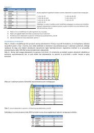
the information about the real world is given in the form of an informationtable (sometimes called a decision table).Thus, the information table represents input data, gathered from any domain,such as medicine, finance, or the military.Rows of a table, labeled e1, e2, e3, e4, e5, and e6 are called examples(objects, entities).

Rows of a table, labeled e1, e2, e3, e4, e5, and e6 are called examples(objects, entities).Conditional attributes= {Headache, muscle_pain, temperature}Decisional attribute= {Flu}

Introduction• Rough set theory proposes a new mathematical approach to imperfectknowledge, i.e. to vagueness (or imprecision). In this approach, vaguenessis expressed by a boundary region of a set.• Rough set concept can be defined by means of topological operations,interior and closure, called approximations.

Information Systems/Tables• IS is a pair (U, A)• U is a non-empty finite set of objects.• A is a non-empty finite set of attributes such thatfor every a A. a : U V aV a• is called the value set of a.

Decision Systems/Tables• DS: T ( U,A{d})• d A is the decision attribute (instead of one we canconsider more decision attributes).• The elements of A are called the condition attributes.

Indiscernibility• The equivalence relationA binary relationR X Xwhich is– reflexive (xRx for any object x) ,– symmetric (if xRy then yRx), and– transitive (if xRy and yRz then xRz).[x] R• The equivalence classx Xconsists of all objectsof an elementy Xsuch that xRy.

Indiscernibility (2)• Let IS = (U, A) be an information system, then with any B Athereis an associated equivalence relation:IND IS( B){(x,x')U2| aB,a(x) a(x')}where IND IS(B) is called the B-indiscernibility relation.• If ( x,x') INDIS( B),then objects x and x’ are indiscernible from eachother by attributes from B.• The equivalence classes of the B-indiscernibility relation aredenoted by x].[B

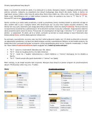
The set consisting of attributes Headache and Muscle_pain:IND({Headache,Muscle_pain})={{e1,e2,e3},{e4,e6},{e5}}Examples e1 and e2 are characterized by the same values of both attributes: for theattribute Headache the value is yes for e1 and e2 and for the attribute Muscle_painthe value is yes for both e1 and e2.Moreover, example e3 is indiscernible from e1 and e2.Examples e4 and e6 are also indiscernible from each other.Obviously, the indiscernibility relation is an equivalence relation.Sets that are indiscernible are called elementary sets.

Thus, the set of attributes Headache and Muscle_pain defines the followingelementary sets: {e1, e2, e3}, {e4, e6}, and {e5}.Any finite union of elementary sets is called a definable set.In our case, set {e1, e2, e3, e5} is definable by the attributes Headache andMuscle_pain, since we may define this set by saying that any member of itis characterized by the attribute Headache equal to yes and the attributeMuscle_pain equal to yes or by the attribute Headache equal to no and theattribute Muscle_pain equal to no.

An Example of Indiscernibility• The non-empty subsets of the condition attributes are {Hedeache}, {Muscle_pain},{Temperature} and {Hedeache,Muscle_pain}, {Hedeache,Temperature},{Muscle_pain,Temperature} , {Hedeache,Temperature ,Muscle_pain}.• IND({Hedeache}) = {{e1,e2,e3}, {e4,e5,e6}}• IND({Muscle_pain}) = {{e1,e2,e3,e4,e6},{e5}}• IND({Temperature}) ={{e1,e4},{e2,e5},{e3,e6}}• IND({Hedeache, Muscle_pain}) = {{e1,e2,e3}, {e4,e6},{e5}}• IND({Muscle_pain, Temperature}) = {{e1,e4},{e2},{e3,e6},{e5}}• IND({Hedeache,Temperature}) ={{e1}{e2},{e3},{e4},{e5},{e6}}• IND({Hedeache,Temperature, Muscle_pain}) ={{e1}{e2},{e3},{e4},{e5},{e6}}

Observations• An equivalence relation induces a partitioning ofthe universe.• Subsets that are most often of interest have thesame value of the decision attribute.

Set Approximation• Let T = (U, A) and let B A and X U.We canapproximate X using only the information contained in Bby constructing the B-lower and B-upper approximationsof X, denoted B X and respectively, whereBXBXBX{ x |[ x]X},B{ x |[ x] X }.B

Set Approximation (2)• B-boundary region of X,BN B( X ) BX BX,consists of those objects that we cannot decisively classifyinto X in B.• B-outside region of X, U BX , consists of those objectsthat can be with certainty classified as not belonging to X.• A set is said to be rough if its boundary region is nonempty,otherwise the set is crisp.

An Example of Set Approximation• Let W = {x | Walk(x) = yes}.AW{ x1,x6},AWBNUA { x1,x3,x4,x6},( WAW) { x3,x4}, { x2,x5,x7}.• The decision class, Walk, isrough since the boundaryregion is not empty.

An Example ofSet Approximation (2){{x2}, {x5,x7}}AW{{x3,x4}}AW{{x1},{x6}}yesyes/nono

Lower & Upper ApproximationsUpper Approximation:(2)RX{ Y U/ R : Y X }Lower Approximation:RX { Y U/ R : Y X}

Rough Membership Function• Rough sets can be also defined by using, instead of approximations, a roughmembership Function.• In classical set theory, either an element belongs to a set or it does not.• The corresponding membership function is the characteristic function for theset, i.e. the function takes values 1 and 0, respectively. In the case of rough sets,the notion of membership is different.• The rough membership function quantifies the degree of relative overlapbetween the set X and the equivalence class R(x) to which x belongs. It is definedas follows.

The meaning of rough membership function

ough membership function• The rough membership function expresses conditional probabilitythat x belongs to X given R and can be interpreted as a degree thatx belongs to X in view of information about x expressed by R.• The rough membership function can be used to defineapproximations and the boundary region of a set:

Problems with real life decisionsystems• A decision system expresses all the knowledge about the model.• This table may be unnecessarily large in part because it isredundant in at least two ways.• The same or indiscernible objects may be represented severaltimes, or some of the attributes may be superfluous.

An example• Let X = {x :Walk(x)= Yes}• In fact, the set X consists of three objects: x1,x4,x6.• Now, we want to describe this set in terms of the set ofconditional attributes A ={Age, LEMS}.Using the above definitions, we obtain the followingapproximations:the A-lower approximation AX = {x1,x6}the A-upper approximation AX = {x1, x3, x4, x6}the A-boundary region BN S (X)={x3, x4},and the A-outside region U − AX = {x2, x5, x7}It is easy to see that the set X is rough since the boundary region is not empty.

Indiscernibility relationAn indiscernibility relation is the main concept of rough settheory, normally associated with a set of attributes.

Accuracy of Approximation B( X ) | B(X| B(X) |) |where |X| denotes the cardinality ofObviously 0 B1.If B( X ) 1,X is crisp with respect to B.If ( X ) 1,X is rough with respect to B. BX .

Issues in the Decision Table• The same or indiscernible objects may berepresented several times.• Some of the attributes may be superfluous(redundant).That is, their removal cannot worsen theclassification.

Reducts• Keep only those attributes that preserve theindiscernibility relation and, consequently, setapproximation.• There are usually several such subsets ofattributes and those which are minimal arecalled reducts.

LetDispensable & IndispensableAttributesAttribute c is dispensable in TifPOScC.C( D) POS ( C{c})( D), otherwiseattribute c is indispensable in T.The C-positive region of D:POSC( D)XU/ DCX

Independent• T = (U, C, D) is independentif all are indispensable in T.cC

Reduct & Core• The set of attributes R C is called a reduct of C,if T’ = (U, R, D) is independent andPOS ( D) POS ( D).RC• The set of all the condition attributesindispensable in T is denoted by CORE(C).CORE ( C) RED(C)where RED(C) is the set of all reducts of C.

Due to the concept of indiscernibility relation, it is very simple to defineredundant (or dispensable) attributes.If a set of attributes and its superset define the same indiscernibility relation(i.e., if elementary sets of both relations are identical), then any attributethat belongs to the superset and not to the set is redundant.In the example let the set of attributes be the set {Headache, Temperature}and its superset be the set of all three attributes, i.e., the set {Headache,Muscle_pain, Temperature}.

Elementary sets of the indiscernibility relation defined by the set {Headache,Temperature} are singletons, i.e., sets {e1}, {e2}, {e3}, {e4}, {e5}, and {e6},and so are elementary sets of the indiscernibility relation defined by theset of all three attributes.Thus, the attribute Muscle_pain is redundant. On the other hand, the set{Headache, Temperature} does not contain any redundant attribute, sinceelementary sets for attribute sets {Headache} and {Temperature} are notsingletons. Such a set of attributes, with no redundant attribute, is calledminimal (or independent).The set P of attributes is the reduct (or covering) of another set Q ofattributes if P is minimal and the indiscernibility relations, defined by Pand Q, are the same (the last condition says that elementary sets,determined by indiscernibility relations defined by P and Q, areidentical).

In our example, the set {Headache, Temperature} is a reduct of the originalset of attributes {Headache, Muscle_ pain, Temperature}.Table 2 presents a new information table based on this reduct.

What about the decision attribute ?We can define elementary sets associated with the decision as subsets of the set ofall examples with the same value of the decision.Such subsets will be called concepts.For Tables 1 and 2, the concepts are {e1, e4, e5} and {e2, e3, e6}.The first concept {e1, e4, e5} corresponds to the set of all patients free from flu,the second one {e2, e3, e6} to the set of all patients sick with flu.Q: Whether we may tell who is free from flu and who is sick with flu on the basis ofthe values of attributes in Table 2 ?A: We may observe that in terms of rough set theory, decision Flu depends onattributes Headache and Temperature, since all elementary sets ofindiscernibility relation associated with {Headache, Temperature} are subsets ofsome concepts.

Generate the rules from data…As a matter of fact, one may induce the following rules from Table 2:• (Temperature, normal) -> (Flu, no),• (Headache, no) and (Temperature, high) -> (Flu,no),• (Headache, yes) and (Temperature, high) ->(Flu, yes),• (Temperature, very_high) -> (Flu, yes).Suppose we have two additional examples, e7 ande8, as presented in Table 3.Elementary sets of indiscernibility relation defined byattributes Headache and Temperature are {e1}, {e2},{e3}, {e4}, {e5, e7}, and {e6, e8}, while conceptsdefined by decision Flu are {e1, e4, e5, e8} and {e2,e3, e6, e7}.

Obviously, the decision Flu does not depend on attributes Headache andTemperature since neither {e5, e7} nor {e6, e8} are subsets of any concept.In other words, neither concept is definable by the attribute set {Headache,Temperature}.We say that Table 3 is inconsistent because examples e5 and e7 areconflicting (or are inconsistent)—for both examples the value of anyattribute is the same, yet the decision value is different. (Examples e6 ande8 are also conflicting.)

• In this situation, rough set theory offers a tool to deal withinconsistencies.• The idea is very simple—for each concept X the greatest definable setcontained in X and the least definable set containing X are computed.• The former set is called a lower approximation of X; the latter is calledan upper approximation of X.• In the case of Table 3, for the concept {e2, e3, e6, e7}, describingpeople sick with flu, the lower approximation is equal to the set {e2,e3}, and the upper approximation is equal to the set {e2, e3, e5, e6,e7, e8}.

Lower and upper approximations of set X

Rules generated from lower andupper approximationFor any concept, rules induced from its lower approximation are certainlyvalid (hence such rules are called certain). Rules induced from the upperapproximation of the concept are possibly valid (and are called possible).For Table 3, certain rules are:(Temperature, normal) -> (Flu, no),(Headache, yes) and (Temperature, high) -> (Flu, yes),(Headache, yes) and (Temperature, very_high) -> (Flu, yes);and possible rules are:(Headache, no) -> (Flu, no),(Temperature, normal) -> (Flu, no),(Temperature, high) -> (Flu, yes),(Temperature, very_high) -> (Flu, yes).

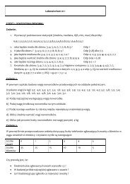
Id colour size Ripe apple ?X1 Red Big YesX2 Yellow Medium YesX3 Green Small NoX4 Green Big YesX5 Yellow Medium NoX6 Red Medium YesX7 Yellow Big YesX8 Red Medium YesX9 Yellow Small NoX10 Yellow Small YesX11 Red Small Yesx12 green medium NobigmediumsmallRed yellow green

Id colour size Ripe apple ?X1 Red Big YesX2 Yellow Medium YesX3 Green Small NoX4 Green Big YesX5 Yellow Medium NoX6 Red Medium YesX7 Yellow Big YesX8 Red Medium YesX9 Yellow Small NoX10 Yellow Small YesX11 Red Small Yesx12 green medium NobigmediumsmallX – ripe appleX – NOT ripe appleRed yellow green

ipe appleId colour size Ripe apple ?X1 Red Big YesX2 Yellow Medium YesX3 Green Small NoX4 Green Big YesX5 Yellow Medium NoX6 Red Medium YesX7 Yellow Big YesX8 Red Medium YesX9 Yellow Small NoX10 Yellow Small YesX11 Red Small Yesx12 green medium NobigmediumsmallX – ripe appleX – NOT ripe appleimmatureappleRed yellow green

lower approximation• BX = {Y IND(B): Y X}• So there are the objects that belong to theIND (B), which all are included in the set of X.• About the objects belonging to the lowerapproximation, we say that they SURELYbelong to a given concept (decision class).

BX = {Y IND(B): Y X}IND(B) = {{1},{2,5},{3},{4},{6}}X = X yes + X noWhich of the Ybelonged to IND(B)are all included in X?X yes = {1,2,3,6}X no = {4,5}BX yes = {1,3,6}BX No = {4}Objects {1,3,6} surely have a flu !Object {4} does not have a flue for SURE!

Upper aproximation• BX = {Y IND(B): Y ∩ X }• So they are those objects that belong to theIND (B), which have a common part with set X.• About the objects belonging to the upperapproximation, we say that they perhapsbelong to a given concept (decision class).

BX = {Y IND(B): Y ∩ X }IND(B) = {{1},{2,5},{3},{4},{6}}X = X yes + X noWhich of Y thatbelong to IND(B)have a common partwith X ?X yes = {1,2,3,6}X no = {4,5}BX yes = {1,2,3,6,5}BX No = {2,5,4}Objects {1,2,3,6,5} maybe have a flu !Objects {2,5,4} maybe doesn’t have a flu !

1. if (h=no) and (m=yes) and (t=high) then (f=yes)2. ….….

Deterministic rulesNON -Deterministic rules

Inconsistency• Decisions may be inconsistent because of limited cleardiscrimination between criteria and because of hesitation onthe part of the decision maker.• These inconsistencies cannot be considered as a simple erroror as noise. They can convey important information thatshould be taken into account in the construction of thedecision makers preference model.• The rough set approach is intended to deal with inconsistencyand this is a major argument to support its application tomultiple-criteria decision analysis.

Inconsistent decision tableThe Table is inconsistent because:• examples e5 and e7 are conflicting (or are inconsistent)—forboth examples the value of any attribute is the same, yet thedecision value is different.• Examples e6 and e8 are also conflicting.

How to deal with the inconsistencyThe idea is very simple—for each concept X the greatest definable setcontained in X and the least definable set containing X are computed.The former set is called a lower approximation of X;the latter is called an upper approximation of X.

for the concept {e2, e3, e6, e7}, describing people sick with flu, thelower approximation is equal to the set {e2, e3}, and the upperapproximation is equal to the set {e2, e3, e5, e6, e7, e8}.

• Either of these two concepts is an example of a rough set, aset that is undefinable by given attributes.• The set {e5, e6, e7, e8}, containing elements from the upperapproximation of X that are not members of the lowerapproximation of X, is called a boundary region.• Elements of the boundary region cannot be classified asmembers of the set X.

• For any concept, rules induced from its lower approximation arecertainly valid (hence such rules are called certain).• Rules induced from the upper approximation of the concept arepossibly valid (and are called possible)

Certain rules• (Temperature, normal) -> (Flu, no),• (Headache, yes) and (Temperature, high) -> (Flu, yes),• (Headache, yes) and (Temperature, very_high) -> (Flu, yes);Possible rules• (Headache, no) -> (Flu, no),• (Temperature, normal) -> (Flu, no),• (Temperature, high) -> (Flu, yes),• (Temperature, very_high) -> (Flu, yes).

How to deal with inconsistency?1. Ask the expert „what to do ?”2. Separate the conflicting examples to differenttables3. Remove the examples with less support4. Quality methods – based on lower or upperapproximations5. The method of generating new (general)decision attribute

4th method• 1 step: calculate the accuracy of the lower orupper approximation• 2 step: we remove the examples with the lessvalue of the accuracy

• IND(B) = {{1}{2,5}{3}{4}{6}}• X yes = {1,2,3,6}• X no = {5,4}• BX yes = {1,3,6}• BX No = {4}• yes =3/6• No =1/6Remove the object(s) with less valueof acuracy of the approximationRemove the object that make a conflict hereand are in the set of decision„No”

• IND(B) = {{1}{2,5}{3}{4}{6}}• X yes = {1,2,3,6}• X no = {5,4}• BX yes = {1,3,6}• BX No = {4}• yes =3/6• No =1/6Remove the object(s) with less valueof acuracy of the approximationRemove the object that make a conflict hereand are in the set of decision„No”

Conditional attributes5th method

ule generation algorithmAuthors: Andrzej Skowron, 1993The algorithm which find in the set of examplesthe set of minimal certain decision rules

Discernibility matrix

Discernibility Matrices andFunctionsIn order to compute easily reducts and the corewe can use discernibility matrix, which isdefined below.

Discernibility functionA prime implicant is a minimal implicant (with respect to the number of its literals). Here we are interested in implicants ofmonotone Boolean functions only, i.e. functions constructed without negation.

In this table H,M,T,Fdenote Headache,Muscle-pain,Temperature and Flu,respectively.The discernibility functionfor this table is• where ∨ denotes the disjunction and theconjunction is omitted in the formula.

DM -> reduct• After simplification, the discernibility function using lawsof Boolean algebra we obtain the following expressionHTF, which says that there is only one reduct {H,T,F} inthe data table and it is the core.• Relative reducts and core can be computed also using thediscernibility matrix, which needs slight modification.

Deterministic DT

Dissimilarity functionsp1 p2 p3 p4 P6P1P2 H,MP3 H,T M,TP4 T H,M,T H,Tp6 T H,M,T H T

Which examples have different decision ?exampleP1P2P3P4p6Different decisionP4P4P4P1,p2,p3,p4P4

Dissimilarity function for p1exampleP1P2P3P4p6Different decisionP4P4P4P1,p2,p3,p4P4p1 p2 p3 p4 P6P1P2 H,MP3 H,T M,TP4 T H,M,T H,Tp6 T H,M,T H Tf( p1,{yes})t

Dissimilarity function for p2exampleP1P2P3P4p6Different decisionP4P4P4P1,p2,p3,p4P4p1 p2 p3 p4 P6P1P2 H,MP3 H,T M,TP4 T H,M,T H,Tp6 T H,M,T H Tf( p2,{yes})hmt

Dissimilarity function for p3exampleP1P2P3P4p6Different decisionP4P4P4P1,p2,p3,p4P4p1 p2 p3 p4 P6P1P2 H,MP3 H,T M,TP4 T H,M,T H,Tp6 T H,M,T H Tf( p3,{yes})ht

Dissimilarity function for p6exampleP1P2P3P4p6Different decisionP4P4P4P1,p2,p3,p4P4p1 p2 p3 p4 P6P1P2 H,MP3 H,T M,TP4 T H,M,T H,Tp6 T H,M,T H Tf( p6,{yes})t

Dissimilarity function for p4exampleP1P2P3P4p6Different decisionP4P4P4P1,p2,p3,p4P4p1 p2 p3 p4 P6P1P2 H,MP3 H,T M,TP4 T H,M,T H,Tp6 T H,M,T H Tf( p4,{no}) t (hmt)(ht)tt

f(p1,{yes})tTemperature = high flu = yes

f( p2,{yes})hmtheadache = yes flu = yesMuscle-pain = no flu = yesTemperature = hight flu = yes

f( p3,{yes})htheadache = yes flu = yesTemperature = very hight flu = yes

f( p6,{yes})tTemperature = hight flu = yes

f( p4,{no}) t (hmt)(ht)ttTemperature = normal flu = no

Temperature = high flu = yesTemperature = high flu = yesheadache = yes flu = yesMuscle-pain = no flu = yesTemperature = hight flu = yesTemperature = high flu = yesheadache = yes flu = yesTemperature = very hight flu = yesTemperature = normal flu = no

Temperature = high flu = yesTemperature = high flu = yesheadache = yes flu = yesMuscle-pain = no flu = yesTemperature = hight flu = yesTemperature = high flu = yesheadache = yes flu = yesTemperature = very hight flu = yesTemperature = normal flu = no

Final set of rulesTemperature = high flu = yesheadache = yes flu = yesMuscle-pain = no flu = yesheadache = yes flu = yesTemperature = very hight flu = yesTemperature = normal flu = no

• Rough set theory offers effective methods that are applicable inmany branches of AI.• One of the advantages is that programs implementing its methodsmay easily run on parallel computers.

Advantages of Rough Set approach• It provides efficient methods, algorithms and tools for findinghidden patterns in data.• It allows to reduce original data, i.e. to find minimal sets ofdata with the same knowledge as in the original data.• It allows to generate in automatic way the sets of decisionrules from data.• It is easy to understand.