Genetics of gene expression: 2010 lab - Bioconductor

Genetics of gene expression: 2010 labVJ CareyJuly 28, 2010Contents1 eQTL concepts and discovery tools 21.1 Checking for informative variants for a specified gene . . . . . . . . . . . 31.2 Components of the workflow; refinements . . . . . . . . . . . . . . . . . . 41.2.1 Data representation: smlSet . . . . . . . . . . . . . . . . . . . . . 61.2.2 Analysis: snp.rhs.tests; permutation testing . . . . . . . . . . . 81.2.3 Context: GenomicRanges and rtracklayer . . . . . . . . . . . . . 92 Comprehensive eQTL surveys: performance issues 112.1 A study of genes coresident on chromosome 20 . . . . . . . . . . . . . . . 112.2 Expanding to genes on multiple chromosomes . . . . . . . . . . . . . . . 132.3 Exercises . . . . . . . . . . . . . . . . . . . . . . . . . . . . . . . . . . . . 153 Investigating allele-specific expression with RNA-seq data 173.1 The data . . . . . . . . . . . . . . . . . . . . . . . . . . . . . . . . . . . . 173.2 Filtering to “coding SNP”; checking for de novo variants . . . . . . . . . . 183.3 Assessing allelic imbalance in transcripts harboring SNPs . . . . . . . . . 203.4 Checking consistency of findings with GENEVAR expression arrays . . . 233.5 Exercises . . . . . . . . . . . . . . . . . . . . . . . . . . . . . . . . . . . . 244 Appendix: samtools pileup format, from samtools distribution site 255 Session information 261

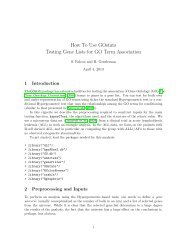
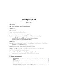
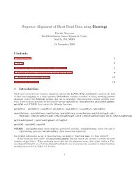
Figure 1: A schematic illustrating various nonexclusive mechanisms by which DNAvariants can affect transcript abundance (Williams et al., 2007).1 eQTL concepts and discovery toolsThe basic concern in the lab is the relationship between structural variation in DNA andvariation in mRNA abundance. DNA variants of interest are primarily SNP as identifiedthrough• direct genotyping in the Sanger sequencing paradigm (yielding HapMap phase IIgenotypes, for example)• array-based genotyping (yielding HapMap phase III)• NGS-based variant calling (as provided for 1000 genomes (1KG))• hybrids of array-based and imputed genotypes (imputation to the 1KG panel)mRNA variation is typically characterized using gene expression microarrays, but RNAseqcan also be considered.A helpful schematic indicating possible impacts of structural variation on gene transcriptionis given in Williams et al. (2007); see Figure 1.2

To elucidate impacts of DNA variations on regulation of gene transcription we needto be able to• represent mRNA abundance and SNP genotypes (both observed and imputed) ina coordinated way for many samples• perform suitably focused and calibrated tests of association between mRNA levelsand genotype (e.g., allele count for a SNP)• provide significance assessments and functional contexts for observed associations.On the basis of excellent algorithms and software in the snpMatrix package of Claytonand Leung (Clayton and Leung, 2007)), the GGtools package provides tools to addressall of these concerns.1.1 Checking for informative variants for a specified geneThe following is a simple illustration of a focused workflow.> library(GGtools)Loading package ff 2.1-2- getOption("fftempdir")=="/var/folders/4D/4DI98FkjGzq0K2niUTEHSE+++TM/-Tmp-//RtmpLbQBu- getOption("ffextension")=="ff"- getOption("ffdrop")==TRUE- getOption("fffinonexit")==TRUE- getOption("ffpagesize")==65536- getOption("ffcaching")=="mmnoflush" -- consider "ffeachflush" if your system stalls- getOption("ffbatchbytes")==16777216 -- consider a different value for tuning your sysAttaching package ff> if (!exists("hmceuB36.2021")) data(hmceuB36.2021)> f1 = gwSnpTests(genesym("CPNE1") ~ male, hmceuB36.2021, chrnum(20))> topSnps(f1)p.valrs17093026 6.485612e-14rs1118233 1.897898e-13rs2425078 2.426168e-13rs1970357 2.426168e-13rs12480408 2.426168e-13rs6060535 2.426168e-13rs11696527 2.426168e-13rs6058303 2.426168e-13rs6060578 2.426168e-13rs7273815 2.544058e-133

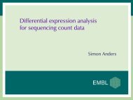
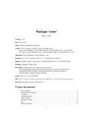
These findings can be visualized in the context of the chromosome in a so-calledManhattan plot; see Figure 2.1.2 Components of the workflow; refinementsThe primary workhorse thus far is gwSnpTests. We need to understand its interface andits return values.> showMethods("gwSnpTests")Function: gwSnpTests (package GGtools)sym="formula", sms="smlSet", cnum="chrnum", cs="missing"(inherited from: sym="formula", sms="smlSet", cnum="cnumOrMissing", cs="missing")sym="formula", sms="smlSet", cnum="cnumOrMissing", cs="missing"sym="formula", sms="smlSet", cnum="snpdepth", cs="chunksize"sym="formula", sms="smlSet", cnum="snpdepth", cs="missing"> f1cwSnpScreenResult [chr 20 ] for gene CPNE1 [probe GI_23397697-A ]> class(f1)[1] "cwSnpScreenResult"attr(,"package")[1] "GGBase"> getClass(class(f1))Class "cwSnpScreenResult" [package "GGBase"]Slots:Name: .Data chrnum gene psid annotation testTypeClass: list chrnum character character character characterName:Class:call sessionInfocall SessionInfoExtends:Class "gwSnpScreenResult", directlyClass "list", by class "gwSnpScreenResult", distance 2Class "vector", by class "gwSnpScreenResult", distance 3Class "AssayData", by class "gwSnpScreenResult", distance 34

plot(f1)CPNE1●−log10 p Gaussian LM [1df]0 2 4 6 8 10 12● ●●●●●●●●●●●●●●● ●●●●●●●●●●●●●●●●●●●●●●●●●●●●●●●●●●●●●●●●●● ●●0e+00 1e+07 2e+07 3e+07 4e+07 5e+07 6e+07position on chr 20Figure 2: Manhattan plot for chromosome 20 eQTL for CPNE1. The y axis measuresthe significance of association of SNP allele copy number with expression for this gene.The association is measured by a χ 2 (1) statistic transformed to a p-value, which islogarithmically transformed and then multiplied by −10.5

1.2.1 Data representation: smlSetThe smlSet container provides coordinated management of expression, genotype, phenotype,and other metadata in a fashion broadly consistent with the ExpressionSetclass. If X is an smlSet instance then• exprs(X) and pData(X) have familiar roles of extracting a matrix of expressionvalues, and a data.frame of sample-level data• X[,S] subsets the samples according to predicate S• X[probeId(P),] subsets the expression data to probes enumerated in predicate P• X[chrnum(C),] subsets the genotype data to chromosome C• annotation(X) returns the annotation package used for mapping expression probeidentifiersClearly there are two kinds of feature in use here: expression probes and SNPs. Theambiguous handling of the X[G,] idiom has not posed a problem thus far. As thestructure gains wider use, more features may be added to simplify filtering throughbracket-based operations.Operations targeted on the genotype data component include:• smList(X) returns a list of snp.matrix objects, using a byte to encode eachgenotype• MAFfilter(X,...) will remove SNP that fail to meet a minor allele frequencycriterion• GTFfilter(X,...) will remove SNP that fail to meet a minimum genotype frequencycriterionThe GGtools package provides hmceuB36.2021 as a modest-sized exemplar of thesmlSet structure, with HapMap phase II genotype data from chromosomes 20 and 21,and GENEVAR expression data for 90 CEU individuals.> hmceuB36.2021snp.matrix-based genotype set:number of samples: 90number of chromosomes present: 2annotation: illuminaHumanv1.dbExpression data dims: 47293 x 90Phenodata: An object of class "AnnotatedDataFrame"sampleNames: NA06985, NA06991, ..., NA12892 (90 total)6

varLabels and varMetadata description:famid: hapmap family idpersid: hapmap person id...: ...male: logical TRUE if male(7 total)> names(pData(hmceuB36.2021))[1] "famid" "persid" "mothid" "fathid" "sampid" "isFounder"[7] "male"> table(hmceuB36.2021$isFounder)FALSE TRUE30 60The expression data is managed exactly as in an ExpressionSet from Biobase. Thegenotype data has a concise representation. It and its coercions are defined in thesnpMatrix package.> s20 = smList(hmceuB36.2021)[["20"]]> s20A snp.matrix with 90 rows and 119921 columnsRow names: NA06985 ... NA12892Col names: rs4814683 ... rs6090120> as(s20, "matrix")[1:4,1:4] # show rawrs4814683 rs6076506 rs6139074 rs1418258NA06985 03 03 03 03NA06991 02 03 02 02NA06993 01 03 01 01NA06994 01 03 01 01> as(s20, "character")[1:4,1:4]rs4814683 rs6076506 rs6139074 rs1418258NA06985 "B/B" "B/B" "B/B" "B/B"NA06991 "A/B" "B/B" "A/B" "A/B"NA06993 "A/A" "B/B" "A/A" "A/A"NA06994 "A/A" "B/B" "A/A" "A/A"> as(s20, "numeric")[1:4,1:4]7

s4814683 rs6076506 rs6139074 rs1418258NA06985 2 2 2 2NA06991 1 2 1 1NA06993 0 2 0 0NA06994 0 2 0 0Question 1: Use plot_EvG to visualize the specific relationship between expressionand allele copy number for the best result for CPNE1 shown above.Question 2: Create a new smlSet hmff limited to CEU founders and with genotypeshaving minimum genotype frequency at least 5%.Question 3: Test for eQTL for CPNE1 in the filtered structure, saving the resultin f1f for later conversions. Create relevant visualizations.1.2.2 Analysis: snp.rhs.tests; permutation testingThe snpMatrix package supplied various utilities for general analysis of genome-wideassociation studies. gwSnpTests is just a wrapper for the snp.rhs.tests function. Tosee it in action,> SS = (SS class(SS)[1] "snp.tests.glm"attr(,"package")[1] "snpMatrix"> length(names(SS))[1] 119921> sum(is.na(p.value(SS)))[1] 53695> SS[1:4, ]Chi.squared Df p.valuers4814683 0.071165981 1 0.7896466rs6076506 0.002905309 1 0.9570141rs6139074 0.680486311 1 0.4094193rs1418258 0.077548726 1 0.7806472> SS["rs6060535", ]8

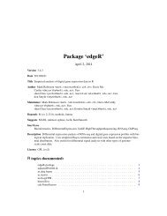
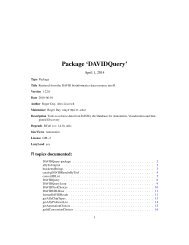
Chi.squared Df p.valuers6060535 53.62528 1 2.426168e-13This shows that for a given phenotypic response, large numbers of GWAS tests can beperformed rapidly.Question 4: Why do so many tests have p-value NA?Which of our findings are significant in the context of so many tests? We can permutethe expression data, keeping the genotype data fixed. Here is one way to obtain a samplefrom the permutation distribution of the smallest p-value for a specific gene.> Mtests = sapply(1:100, function(x) topSnps(gwSnpTests(genesym("CPNE1") ~+ male, sms = permEx(hmceuB36.2021), cnum = chrnum(20)))[[1]][1])1.2.3 Context: GenomicRanges and rtracklayerA major response to the transition to high-throughput sequencing assays is the IRangesinfrastructure. The GenomicRanges package defines the GRanges class, to which we canconvert results of an eQTL search:> gr1 = as(f1, "GRanges")> gr1[1:4, ]GRanges with 4 ranges and 4 elementMetadata valuesseqnames ranges strand | type group score | rs4814683 chr20 [ 9795, 9795] * | snpeff gws 0.10256722rs6076506 chr20 [11231, 11231] * | snpeff gws 0.01908166rs6139074 chr20 [11244, 11244] * | snpeff gws 0.38783167rs1418258 chr20 [11799, 11799] * | snpeff gws 0.10754519universers4814683 hg18rs6076506 hg18rs6139074 hg18rs1418258 hg18seqlengthschr20NA> gr2 = as(f1f, "GRanges")Question 5: Export these GRanges instances as wig files and add to a UCSCbrowser session as custom tracks. You could do this with rtracklayer if your searchlisthad a particular form. You should see something like Figure 3; R Track 1 is the searchon all SNP; R Track 2 follows the restriction to minimum genotype frequency 5%.9

Figure 3: Browser tracks associated with eQTL screens f1 and f1f.10

2 Comprehensive eQTL surveys: performance issuesA comprehensive survey of eQTL would consider possible relationships between 20000or so genes and 8 million or more SNP (the latter is the approximate size of the 1000genomes SNP panel). Creating, storing, and interrogating the family of 160 billion resultsis a significant undertaking. We now illustrate a strategy for conducting comprehensivesurveys.2.1 A study of genes coresident on chromosome 20We will select 50 genes at random from chromosome 20 and compute all tests for associationwith SNP on chromosome 20.First we select the genes and filter the smlSet:> set.seed(1234)> library(illuminaHumanv1.db)> g20 = get("20", revmap(illuminaHumanv1CHR))> samp = sample(g20, size = 50, replace = FALSE)> hlit = hmceuB36.2021[probeId(samp), ]If you are using a POSIX-compliant system, you can speed up this process by distributingover cores. We will be writing data to a folder called dem50.> try(system("rm -rf dem50"))> if (try(require(multicore))) {+ unix.time(e1 unix.time(e1 e1eqtlTools results manager, computed Wed Jul 28 06:50:49 2010There are 2 chromosomes analyzed.some genes: GI_26051259-I GI_42734342-S ... hmm26595-S GI_24041039-Asome snps: rs4814683 rs6076506 ... rs6062370 rs609012011

class(e1)[1] "eqtlTestsManager"attr(,"package")[1] "GGtools"> getClass(class(e1))Class "eqtlTestsManager" [package "GGtools"]Slots:Name: fflist call sess exdate shortfac geneanno dfClass: list call ANY ANY numeric character numericWe are using the ff package to use disk to maintain extremely voluminous outputs.> e1@fflist[[1]][1:4, 1:4]GI_26051259-I GI_42734342-S GI_29570787-I GI_42662261-Srs4814683 86 7 15 1rs6076506 183 71 0 41rs6139074 68 39 1 23rs1418258 101 6 23 1> e1@shortfac[1] 100The information shown above is not intended for public consumption. Instead we performfocused interrogation using brackets and casting:> e1[rsid("rs4814683"), probeId("GI_26051259-I")]$`20`GI_26051259-Irs4814683 0.86Typical use case: finding a collection of strongest associations:> topFeats(probeid = "GI_26051259-I", mgr = e1, ffind = 1, anno = "illuminaHumanv1.db"rs708954 rs237422 rs6017409 rs6065590 rs6107778 rs6030278 rs6120934 rs613969218.56 18.25 16.42 16.06 15.95 15.63 15.56 15.41rs6031075 rs604929914.79 14.6612

topFeats(rsid = "rs708954", mgr = e1, ffind = 1, anno = "illuminaHumanv1.db")KCNQ2 THBD ATRN SRC NFS1 TP53INP2 PFDN4 EMILIN318.56 6.97 5.13 4.13 3.20 2.99 2.86 2.74TCF15 CST22.39 2.19> topFeats(sym = "SRC", mgr = e1, ffind = 1, anno = "illuminaHumanv1.db")rs6063909 rs293554 rs293558 rs293559 rs293544 rs293543 rs293553 rs614131923.88 18.09 18.09 18.09 17.42 17.31 17.28 16.84rs1022732 rs491124216.84 16.842.2 Expanding to genes on multiple chromosomesThe analysis conducted just above uses genes on chromosome 20. We repeat with somegenes on chromosome 21. First sample the genes:> g21 = get("21", revmap(illuminaHumanv1CHR))> samp21 = sample(g21, size = 50, replace = FALSE)> hlit21 = hmceuB36.2021[probeId(samp21), ]Now perform the tests, using a different target folder:> try(system("rm -rf dem50.21"))> unix.time(e2 e2eqtlTools results manager, computed Wed Jul 28 06:51:13 2010There are 2 chromosomes analyzed.some genes: GI_20357564-S GI_21536427-S ... GI_21040313-I GI_31342650-Ssome snps: rs4814683 rs6076506 ... rs6062370 rs6090120To facilitate interrogation of the two sets of results simultaneously, the eqtlTestsManagerinstances need to be coordinated by a cisTransDirector instance.> try(system("rm -rf d2021_probetab.ff"))> try(system("rm -rf d2021_snptab.ff"))> d1 = mkCisTransDirector(list(e1, e2), "d2021", "snptab", "probetab",+ "illuminaHumanv1.db")> d113

eqtlTools cisTransDirector instance.there are 2 managers.Total number of SNP: 170086 ; total number of genes: 100First:eqtlTools results manager, computed Wed Jul 28 06:50:49 2010There are 2 chromosomes analyzed.some genes: GI_26051259-I GI_42734342-S ... hmm26595-S GI_24041039-Asome snps: rs4814683 rs6076506 ... rs6062370 rs6090120---use [ (rsnumvec), (geneidvec) ] to obtain chisq stats; topFeats(), etc.> d1["rs6090120", "GI_42734342-S"]GI_42734342-Srs6090120 0You are now managing and interrogating 170 million test results. By increasing thenumbers of genes and SNP held in the smlSet instances passed to eqtlTests you canincrease this. Interfaces need further refinement.14

3 Investigating allele-specific expression with RNAseqdataWe consider a study of read mapping bias in RNA-seq (Degner et al., 2009). We willconsider how to identify SNPs located in exons, how to analyze allele frequencies for suchSNP, and how to check findings against existing sequencing data and eQTL statisticsfor a single individual and a HapMap population.3.1 The dataWe will use a samtools pileup representation of RNA-seq data that were aligned usingMAQ and distributed by Degner and colleagues through GEO. We confine attention tochromosome 6 for individual NA19238, and use the “unmasked” alignment files. Datafrom two sequencing runs was combined using samtools merge, and then the pileup wasgenerated against hg18.> library(GGtools)> library(Rsamtools)> pup238_6 = readPileup(system.file("pup/combn238_chr6.pup", package = "GGtools"),+ variant = "SNP")> pup238_6[1:4, ]GRanges with 4 ranges and 6 elementMetadata valuesseqnames ranges strand | referenceBase consensusBase | [1] chr6 [40376, 40376] * | C A[2] chr6 [43893, 43893] * | A C[3] chr6 [84124, 84124] * | T C[4] chr6 [84125, 84125] * | G AconsensusQuality snpQuality maxMappingQuality coverage [1] 4 4 0 1[2] 4 4 0 1[3] 4 4 0 1[4] 4 4 0 1seqlengthschr6NAIt will be useful to have the specific pileup of calls as well.> getPupCalls = function(pupfn) {+ tmp = strsplit(readLines(pupfn), "\t")17

+ sapply(tmp, "[", 9)+ }> callp = getPupCalls(system.file("pup/combn238_chr6.pup", package = "GGtools"))> elementMetadata(pup238_6)$callp = callp> pup238_6[144:148, ]GRanges with 5 ranges and 7 elementMetadata valuesseqnamesranges strand | referenceBase consensusBase | [1] chr6 [249623, 249623] * | C A[2] chr6 [249625, 249625] * | T A[3] chr6 [249662, 249662] * | G A[4] chr6 [256482, 256482] * | C T[5] chr6 [256873, 256873] * | C TconsensusQuality snpQuality maxMappingQuality coverage callp [1] 25 25 27 3 ^6A^?A^?A[2] 60 60 38 11 AAAAAAAAAA^UA[3] 33 33 56 2 A$A[4] 4 4 0 1 T[5] 4 4 40 1 ^Itseqlengthschr6NA3.2 Filtering to “coding SNP”; checking for de novo variantsWe have derived a GRanges instance with addresses of exons on chromosome 6, usingthe GenomicFeatures facilities for extracting feature data from UCSC tables.> library(GenomicFeatures)> data(ex6)> ex6[1:4, ]GRanges with 4 ranges and 1 elementMetadata valueseqnames ranges strand | exon_id | [1] chr6 [237101, 237560] + | 81518[2] chr6 [249628, 249661] + | 81519[3] chr6 [256880, 256962] + | 81520[4] chr6 [280114, 280163] + | 8152118

seqlengthschr1 chr1_random chr10 ... chrX_random chrY247249719 1663265 135374737 ... 1719168 57772954> exp_6 = pup238_6[which(ranges(pup238_6) %in% ranges(ex6)), ]How many of the SNP variants in this individual reside in exons? Restrict the pileupdata to these.> sum(ranges(pup238_6) %in% ranges(ex6))[1] 6544> isExonic = which(ranges(pup238_6) %in% ranges(ex6))> pup238_6x = pup238_6[isExonic, ]How many of these exonic variants are already catalogued in the May 2009 dnSNPdatabase?> library(SNPlocs.Hsapiens.dbSNP.20090506)> s6 = getSNPlocs("chr6")> s6[1:5, ]RefSNP_id alleles_as_ambig loc1 6922869 Y 925962 6905277 S 926463 71545186 M 927244 71545187 M 929095 6923601 Y 92941> knownLocs = IRanges(s6$loc, s6$loc)> indbsnp = ranges(pup238_6x) %in% knownLocs> sum(indbsnp)[1] 1266What are the heterozygosity frequencies at known and potentially novel SNP locations?> p6xknown = pup238_6x[which(indbsnp), ]> p6xnovel = pup238_6x[-which(indbsnp), ]> nKnown = length(p6xknown)> nhetKnown = sum(!(elementMetadata(p6xknown)$consensusBase %in%+ c("A", "C", "G", "T")))> nhetKnown/nKnown19

[1] 0.3041074> nNovel = length(p6xnovel)> nhetNovel = sum(!(elementMetadata(p6xnovel)$consensusBase %in%+ c("A", "C", "G", "T")))> nhetNovel/nNovel[1] 0.030693443.3 Assessing allelic imbalance in transcripts harboring SNPsWhat exactly are we looking for? A guide is available through the table published byDegner et al.> data(degnerASE01)> antab = with(degnerASE01, degnerASE01[chr == "chr6" & indiv ==+ "GM19238", 1:8])> antabrsnum refreads nonrefreads miscall chr loc gene indiv2 rs1042448 72 4 0 chr6 33162320 HLA-DPB1 GM1923829 rs3025040 56 133 7 chr6 43861029 VEGFA GM1923846 rs7192 212 317 0 chr6 32519624 HLA-DRA GM1923848 rs7739387 4 32 0 chr6 34730399 C6orf106 GM1923850 rs8084 388 518 2 chr6 32519013 HLA-DRA GM19238This shows 5 loci related to 4 genes for which there is evidence of allele-specific expression,in that the individual is heterozygous at the locus, but the transcript abundancemeasures are skewed towards one of the two alleles present.To check for this on the basis of our pileup data, we have a little tabulation function:> tabCalls = function(pup, ind) {+ ac = as.character+ empup = elementMetadata(pup)+ ref = ac(empup$referenceBase[ind])+ maqcall = ac(empup$consensusBase[ind])+ puptag = gsub("\\^.", "", empup$callp[ind])+ list(ref = ref, maqcall = maqcall, calls = table(strsplit(puptag,+ "")))+ }In the following, we tind overlaps between our exonic loci and the tabulated locations,and tabulate the available calls. First we build a little utility that returns nucleotidesgiven an ambiguous code.20

library(Biostrings)> decodeIU = function(x) {+ if (length(x) > 1)+ warning("only handling first entry")+ strsplit(IUPAC_CODE_MAP[toupper(x)], "")[[1]]+ }Now we identify those locations from the Degner table that coincide with our pileupbasedranges. There is an idiosyncratic but intuitive matrix result wrapped in S4.> ol = findOverlaps(IRanges(antab$loc, width = 1), ranges(pup238_6x))> olAn object of class "RangesMatching"Slot "matchMatrix":query subject[1,] 2 3678[2,] 3 2207[3,] 4 2874[4,] 5 2206Slot "DIM":[1] 5 6544In the following, we generate a little report to summarize the comparisons.> for (i in 1:nrow(ol@matchMatrix)) { # ONEOFF+ cat("query", i, "\n")+ print(t1

query 1rsnum refreads nonrefreads miscall chr loc gene indiv29 rs3025040 56 133 7 chr6 43861029 VEGFA GM19238$ , . T g t1 3 5 10 1 9Degner refFreq = 0.2963Pileup refFreq = 0.2963---query 2rsnum refreads nonrefreads miscall chr loc gene indiv46 rs7192 212 317 0 chr6 32519624 HLA-DRA GM19238$ , . G g11 161 56 83 242Degner refFreq = 0.4008Pileup refFreq = 0.4004---query 3rsnum refreads nonrefreads miscall chr loc gene indiv48 rs7739387 4 32 0 chr6 34730399 C6orf106 GM19238, . C c2 1 11 5Degner refFreq = 0.1111Pileup refFreq = 0.1579---query 4rsnum refreads nonrefreads miscall chr loc gene indiv50 rs8084 388 518 2 chr6 32519013 HLA-DRA GM19238$ , . C c g t12 327 69 127 429 1 1Degner refFreq = 0.4283Pileup refFreq = 0.416---The correspondence is very close. Unfortunately there is relatively low coverage for themost extreme imbalances.22

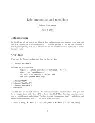
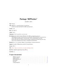
3.4 Checking consistency of findings with GENEVAR expressionarraysThe hmyriB36 package of Bioconductor’s experimental data archive includes expressionand genotyping data on 90 YRI individuals including NA19238. The expression dataare distributed by the GENEVAR project (Stranger et al., 2007).> library(hmyriB36)> if (!exists("hmyriB36")) data(hmyriB36)> library(illuminaHumanv1.db)> pidVEGFA = get("VEGFA", revmap(illuminaHumanv1SYMBOL))> ve = exprs(hmyriB36)[pidVEGFA, "NA19238"]The following code can be used to check for relationship between allele copy number fora SNP and array-based expression values:> plot_EvG(genesym("VEGFA"), rsid("rs3025040"), hmyriB36)> abline(h = ve)●VEGFA6.0 6.1 6.2 6.3 6.4●●●●●●●●●●●●●●●●●●●●●●●●●●●●●●●●●●●●●●●●●●●●●●●●●●●●●●● ●●A/A A/B B/Brs302504023

3.5 ExercisesQuestion 8. Check the array-based expression configurations for the other four geneswith potential allele-specific expression.Question 9. Write code that scans all the exonic SNP on chr6 and identifies lociwith potential imbalance. You might modify the code snippet marked ONEOFF above.What statistical tests and multiple testing corrections should you use?Question 10. Acquire the data on NA19239 and reproduce some of the key entriesof the Degner table.24

4 Appendix: samtools pileup format, from samtoolsdistribution sitePileup FormatPileup format is first used by Tony Cox and Zemin Ning at the SangerInstitute. It describes the base-pair information at each chromosomalposition. This format facilitates SNP/indel calling and brief alignmentviewing by eyes.The pileup format has several variants. The default output by SAMtools looks like this:seq1 272 T 24 ,.$.....,,.,.,...,,,.,..^+.

5 Session information> toLatex(sessionInfo())• R version 2.12.0 Under development (unstable) (2010-06-30 r52417),x86_64-apple-darwin10.3.0• Locale: C• Base packages: base, datasets, grDevices, graphics, methods, splines, stats, tools,utils• Other packages: AnnotationDbi 1.11.1, Biobase 2.9.0, Biostrings 2.17.26,DBI 0.2-5, GGBase 3.9.2, GGtools 3.7.33, GenomicFeatures 1.1.6,GenomicRanges 1.1.15, IRanges 1.7.14, RCurl 1.4-2, RSQLite 0.9-1,Rsamtools 1.1.10, SNPlocs.Hsapiens.dbSNP.20090506 0.99.1, annotate 1.27.0,bit 1.1-4, bitops 1.0-4.1, codetools 0.2-2, digest 0.4.2, ff 2.1-2, hmyriB36 0.99.4,illuminaHumanv1.db 1.6.0, multicore 0.1-3, multtest 2.5.0, org.Hs.eg.db 2.4.1,rtracklayer 1.9.3, snpMatrix 1.13.1, survival 2.35-8, weaver 1.15.0• Loaded via a namespace (and not attached): BSgenome 1.17.5,GSEABase 1.11.1, KernSmooth 2.23-3, MASS 7.3-6, XML 3.1-0, annaffy 1.21.0,biomaRt 2.5.1, graph 1.27.10, xtable 1.5-626

ReferencesDavid Clayton and Hin-Tak Leung. An r package for analysis of whole-genome associationstudies. Hum Hered, 64(1):45–51, Jan 2007. doi: 10.1159/000101422.J Degner, J Marioni, A Pai, J Pickrell, E Nkadori, Y Gilad, and J Pritchard. Effect ofread-mapping biases on detecting allele-specific expression from rna-sequencing data.Bioinformatics, Oct 2009. doi: 10.1093/bioinformatics/btp579.Barbara E Stranger, Alexandra C Nica, Matthew S Forrest, Antigone Dimas, Christine PBird, Claude Beazley, Catherine E Ingle, Mark Dunning, Paul Flicek, Daphne Koller,Stephen Montgomery, Simon Tavaré, Panos Deloukas, and Emmanouil T Dermitzakis.Population genomics of human gene expression. Nat Genet, 39(10):1217–24, Oct 2007.doi: 10.1038/ng2142.R. B.H Williams, E. K.F Chan, M. J Cowley, and P. F.R Little. The influence of geneticvariation on gene expression. Genome Research, 17(12):1707–1716, Dec 2007. doi:10.1101/gr.6981507.27