Nonlinear Attitude and Position Control of a Micro Quadrotor using ...

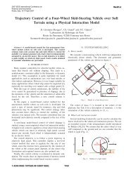
3rd US-European Competition and Workshop on Micro Air Vehicle Systems (MAV07) & European Micro Air VehicleConference and Flight Competition (EMAV2007), 17-21 September 2007, Toulouse, FranceNonlinear Attitude and Position Control of a MicroQuadrotor using Sliding Mode and BacksteppingTechniquesPatrick Adigbli ∗Technische Universität München, 80290 München, Germany andChristophe Grand † and Jean-Baptiste Mouret ‡ and Stéphane Doncieux §ISIR, Institut des Systèmes Intelligents et Robotique, 75016 Paris, FranceThe present study addresses the issues concerning the developpment of a reliable assistedremote control for a four-rotor miniature aerial robot (known as quadrotor), guaranteeingthe capability of a stable autonomous flight. The following results are proposed: afterestablishing a dynamical flight model as well as models for the rotors, gears and motorsof the quadrotor, different nonlinear control laws are investigated for attitude and positioncontrol of the UAV. The stability and performance of feedback, backstepping andsliding mode controllers are compared in simulations. Finally, experiments on a newlyimplemented quadrotor prototype have been conducted in order to validate the theoreticalanalysis.I. IntroductionAs their application potential both in the military and industrial sector strongly increases, miniatureunmanned aerial vehicles (UAV) constantly gain in interest among the research community. Mostlyused for surveillance and inspection roles, building exploration or missions in unaccessible or dangerousenvironments, the easy handling of the UAV by an operator without hours of training is primordial. In orderto develop a reliable assisted remote control or guarantee the capability of a stable autonomous flight, thedevelopment of simple and robust control laws stabilizing the UAV becomes more and more important.This article addresses the design and analysis of nonlinear attitude and position controllers for a four-rotoraerial robot, better known as quadrotor. This aircraft has been chosen for its specific characteristics suchas the possibility of vertical take off and landing (VTOL), stationary and quasi-stationary flight and highmanoeuverability. Moreover, its simple mechanical structure compared to a helicopter with variable pitchangle rotors and its highly nonlinear, coupled and underactuated dynamics make it an interesting researchplatform.The present article proposes the following results: in the second part, models for the propulsion systemand the flight dynamic of the UAV are proposed. In the third part, different nonlinear control laws tostabilize the attitude of the quadrocopter are investigated. In the fourth part, a new position controller forautonomous waypoint tracking is designed, using the backstepping approach. Finally, the performance ofthe investigated controllers are compared in simulations and experiments on a real system. For that purpose,a prototype of the quadrocopter has been implemented.II. Modelling the electromechanical systemIn this section, a complete model of the quadrocopter system is established. First, a model of thepropulsion system represented in Fig.1 is proposed, deriving theoretical linear and nonlinear models for therotor, gear and motor.∗ Master student TUM/ECP, Institute of Automatic Control Engineering, patrick.adigbli@centraliens.net† Prof. assistant, dept SIMA, grand@robot.juiisu.fr‡ PhD student, dept SIMA, Jean-Baptiste.Mouret@lip6.fr§ Prof. assistant, dept SIMA, Stephane.Doncieux@upmc.fr1

3rd US-European Competition and Workshop on Micro Air Vehicle Systems (MAV07) & European Micro Air VehicleConference and Flight Competition (EMAV2007), 17-21 September 2007, Toulouse, FranceThe reactive torque τ R caused by the drag of the rotor bladeand the thrust f are proportional to the square of the rotationalvelocity ω of the rotor (see McKerrow et al. 1 ):f = k l ω 2 , τ R = k d ω 2 (1)The gear is located between the rotor and the couplegeneratingmotor a , in order to transmit the mechanical powerwhile changing the motor couple τ M and the rotational velocityω. Considering the mechanical losses by introducing theefficiency factor η G , the gear reduction ratio G as well as thetotal torque of inertia ˜J tot on the motor side can be calculated:Figure 1. Propulsion system.G = ˜ω ω = τ M˜τ M1η Gand ˜Jtot = J RG 2 + J M (2)The well-known electromechanical model of the dc motor is described by the two following equations,introducing the back-EMF constant k emk and the torsional constant k M :L M ˙i M = ū M − R M i M − k emk ω (3)˜J tot ˙˜ω = ˜τ M − ˜τ R = k M i M − ˜τ R (4)With respect to the fact that the motor inductivity L M can be considered small in comparison to the motorresistance R M , the system dynamic can be reduced. By taking into account the equations (1) and (2), thesimplified nonlinear model for the propulsion system is:˙ω =k MR M G ˜Jū M − k M k emk k dtot R M G ˜Jω − ω 2 (5)tot G 2 η G ˜JtotThe stationary response curve can be linearized around the operating point (ω ∗ ,ū ∗ M ), finally leading to thesimplified and linearized propulsion system model used in this article b :ω = K 1T s + 1 ūM + K 2T s + 1This model has been verified by an experimental analysison the propulsion system, using the Least-Square-Fittingmethod.(6)After proposing the model of the electromechanical propulsionsystem, a simplified quasi-stationary flight dynamic modelbased on the work of Lozano et al. 2 and Bouabdallah andal. 3 will be established. Considering the whole quadrotorsystem represented in Fig.2, the earth-fixed coordinate systemS W = [X,Y ,Z] T and the body-fixed coordinate systemS uav = [x,y,z] T are introduced. The position ξ = [x,y,z] T ofthe UAV is given by the position of the origin of the body-fixedcoordinate system relativ to the origin of the earth coordinateFigure 2. Representation of the quadrotor system,introducing torques, forces and coordinatesystems.system. The orientation of the UAV in space is described by the Tait-Bryan-angles η = [Φ,Θ,Ψ] T and therotation matrix R c :a All variables on the motor side are marked with a tilde, while all variables on the rotor side aren’t marked.b With the parameters:η G G k Mk d ω ∗2 R Mη G G 2 K 1 =2 k d ω ∗ , K 2 =R M + η G G k emk k M 2 k d ω ∗ , T =˜J tot R MR M + η G G k emk k M 2 k d ω ∗ R M + η G G k emk k Mc In this article, the representation of the rotation matrix R is based on the following rotation order: the first rotation withthe angle Φ around the x-axis, the second rotation with the angle Θ around the new y-axis and the third rotation with theangle Ψ around the new z-axis.2

3rd US-European Competition and Workshop on Micro Air Vehicle Systems (MAV07) & European Micro Air VehicleConference and Flight Competition (EMAV2007), 17-21 September 2007, Toulouse, France⎛⎞c Θ c Ψ s Φ s Θ c Ψ − c Φ s Ψ c Φ s Θ c Ψ + s Φ s Ψ⎜⎟R = ⎝c Θ s Ψ s Φ s Θ s Ψ + c Φ c Ψ c Φ s Θ s Ψ − s Φ c Ψ ⎠ (7)−s Θ s Φ c Θ c Φ c ΘThe angular rotation velocities Ω in the body-fixed coordinates can be obtained with respect to theangular rotation velocities ˙η in the earth-fixed coordinates:⎛ ⎞1 0 −s Θ⎜ ⎟Ω = ⎝0 c Φ s Φ c Θ ⎠ ˙η = W(η) ˙η (8)0 −s Φ c Φ c ΘNow, a full dynamical model of the position and angular acceleration of the quadrocopter is derived,showing that the Euler-Lagrange-formalism, which is also used in the work of Lozano et al., 2 leads tothe same results as the Newton-Euler approach used by Bouabdallah et al. 3 Introducing ρ = [ξ,η] T andapplying the Hamilton principle to the Lagrange function L(ρ, ˙ρ) = T (ρ, ˙ρ) − V(ρ) composed of the kineticand potential energies T and V of the global mechanical system leads to the Euler-Lagrange-equations:ddt( ∂L∂ ˙ρ i)− ∂L∂ρ i= Q i with i = 1...6 (9)First, all components of the Lagrange function L and the generalized potential-free force vector Q have tobe identified. Both can be divided in a translational and a rotational part:L trans = T trans − V = 1 2 m ˙ξ)Tuav ˙ξ + muav g z Q trans = R−FL rot = T rot = 1 2 ΩT I Ω = 1 ( )0 l kl 0 −l k l2 ˙ηT J ˙η Q rot = τ + τ gyro = l k l 0 −l k l 0 ω 2k d −k d k d −k d4∑+ J R (Ω × e z )(−1) i+1 ω iNow, the Euler-Lagrange-equations for position and orientation can be deduced independently:( )(Q trans = d ∂L transdt ∂ ˙ξ − ∂Ltrans∂ξ¨ξ = Q 00g)trans( )mQ rot = d ∂Lrot⇔uav ( +dt ∂ ˙η− ∂Lrot∂η¨η = J −1 (Q rot + 1 ∂2 ∂η ˙η T J ˙η ) − ˙J(10)˙η)After considering the hypothesis of small angles and small angular velocities, the full dynamical model(10) can be simplified, resulting in a nonlinear coupled model containing terms for the coriolis forces andgyroscopic torques:Fẍ = −m uav(c Φ c Ψ s Θ + s Φ s Ψ )ÿ = −Fm uav(c Φ s Ψ s Θ − s Φ c Ψ )¨z = −F (c Φ c Θ ) + gm uav¨Φ = τΦI x− JR ΠI x¨Θ = τΘI y+ JR ΠI y¨Ψ = τΨI z+˙Φ ˙ΘIII. Attitude stabilization( 00i=1˙Θ + ˙Θ ˙Ψ˙Φ + ˙Φ ˙Ψ( )Ix−I yI z( )Iy−I zI x( )I z−I xI yIn a next step, different nonlinear control laws for the control torque vector τ ctrl = [τ ctrlΦ,τctrlΘ(11),τctrlΨ ]Tare investigated in order to stabilize the highly nonlinear, underactuated system, even in presence of perturbations.The control architecture represented in Fig.3 remains the same for the different control laws.3

3rd US-European Competition and Workshop on Micro Air Vehicle Systems (MAV07) & European Micro Air VehicleConference and Flight Competition (EMAV2007), 17-21 September 2007, Toulouse, FranceIn order to formally prove the stability of this sliding mode controller, the following two assumptionshave to be verified:1. The system has to reach the sliding manifolds S i after a finite time, independently from the systemsinitial state x 0 .2. The motion along the sliding manifolds S i must have a stable behaviour.In order to verify the second assumption, Utkins equivalent control method will be used: 6 therefore, acontinuous equivalent control variable u eq must exist and verify the condition:min (u) ≤ u eq ≤ max (u) (16)In the sliding mode, u eq replaces u and with (14), we have ṡ(x) = 0 and ṡ(x) = ∂s∂x ẋ = ∂s∂x (f (x) + B u eq).Consequently, the equivalent control is given by:∂s∂x( ) −1 ( ∂su eq = −∂x B ∂s∂x f (x) with ∂s c4/I∂x B = x 0 00 c 5/I y 00 0 c 6/I z)The existence of u eq is guaranteed, because the inverse of ∂s∂xB exists and the components of the termf (x) could become zero only in single isolated points of the state space. Thus, the second assumptionis partially verified, only (16) has to be satisfied. To guarantee this, we consider assumption 1, which isequivalent to finding the so called domain of sliding mode and can be reduced to a stability problem withthe state vector s and the lyapunov function V (s) = sign(s) T s. Considering (14), (17) and (15), thederivative of V is:˙V (s) = −K sign(s) T ∂s∂sB sign(s) − sign(s)T∂x ∂x B u eqBecause ∂s∂x B is positive definite, {the first }term of ˙V is confined{to c min ‖sign(s)‖}2 ≤ sign(s) T ∂s∂x B sign(s) ≤c max ‖sign(s)‖ 2 cwith c min = min 4I x, c5I y, c6cI zand c max = max 4I x, c5I y, c6I zand we have:˙V (s) ≤ −Kc min ‖sign(s)‖ 2 + ‖sign(s) T ‖ ‖ ∂s∂x B‖ ‖u eq‖Outside of the sliding manifolds S i , we have ‖sign(s)‖ ≥ 1, because at least one component s i ≠ 0.Therefore, the derivative of the lyapunov function is negative, when we have:(17)K > ‖ ∂s∂x B‖ ‖u eq‖c min(18)By choosing K according to (18), the domain of sliding mode corresponds to the whole state space,verifying assumption 1. Furthermore, we will now show that (16) ⇔ −K ≤ u eq ≤ +K ⇒ ‖u eq ‖ ≤ K( ) 2 ( ) 2 ( )is satisfied by this choice of K. Considering the Frobeniusnorm ‖ ∂s∂x B‖2 F = c 4I x+c 5I y+c 2,6I zthestability of the sliding mode controller is formally proven, because we have:‖u eq ‖ < Kc min‖ ∂s∂x B‖ F≤ K (19)IV.Position controlAnother main contribution of the present article is the design of a position controller based on thebackstepping approach. The superposition of the position controller over the attitude controller in a cascadearchitecture (shown in Fig.4) enables the robot to perform autonomous waypoint tracking: the operatoror path planner provides the desired values x d ,y d ,z d and Ψ d and the position controller calculates thecorresponding control values Φ ctrl ,Θ ctrl and F ctrl , which represent the set values of the underlying attitude5

3rd US-European Competition and Workshop on Micro Air Vehicle Systems (MAV07) & European Micro Air VehicleConference and Flight Competition (EMAV2007), 17-21 September 2007, Toulouse, Francecontroller. To derive the backstepping position control law, a diffeomorphism transforms the position vectorξ = [x,y,z] T into z-coordinates. This operation will be illustrated using the x-coordinate:z 1 = x − x d , z 2 = ẋ − ẋ d − β 1 (z 1 ),z˙1 = ẋ − ẋ d = z 2 + β 1 (z 1 )By introducing the ( partial lyapunov ) functionsV 1 = 1 2 z2 1 and V 2 = 1 2 z21 + z22 , it is possible todetermine the function β 1 (z 1 ) and two parametersb 1 ,b 2 > 0 such that the derivate V ˙ 2 ≡ − ∑ 2i=1 b izi 2

3rd US-European Competition and Workshop on Micro Air Vehicle Systems (MAV07) & European Micro Air VehicleConference and Flight Competition (EMAV2007), 17-21 September 2007, Toulouse, FranceΦ, Θ, Ψ [deg]403020100-10-20-30-40-50Feedback controller, anglesΦΘΨ0 0.5 1 1.5 2 2.5 3 3.5 4Time [s]Φ, Θ, Ψ [deg]403020100-10-20-30-40-50Backstepping controller, anglesΦΘΨ0 0.5 1 1.5 2 2.5 3 3.5 4Time [s]Φ, Θ, Ψ [deg]403020100-10-20-30-40-50Sliding mode controller, anglesΦΘΨ0 0.5 1 1.5 2 2.5 3 3.5 4Time [s][Nm]τ Φctrl , τΘctrl , τΨctrl0.40.30.20.10-0.1-0.2-0.3Feedback controller, control torquesτ Φctrlτ Θctrlτ Ψctrl-0.40 0.5 1 1.5 2 2.5 3 3.5 4Time [s][Nm]τ Φctrl , τΘctrl , τΨctrl0.40.30.20.10-0.1-0.2-0.3Backstepping control, control torquesτ Φctrlτ Θctrlτ Ψctrl-0.40 0.5 1 1.5 2 2.5 3 3.5 4Time [s][Nm]τ Φctrl , τΘctrl , τΨctrlSliding mode controller, control torques0.4ctrlτ0.3Φctrlτ Θctrl0.2τ Ψ0.10-0.1-0.2-0.3-0.40 0.5 1 1.5 2 2.5 3 3.5 4Time [s]Figure 5. Simulation results of the attitude stabilisation, η d = [0 ◦ , 0 ◦ , 0 ◦ ] T . Top row: angles with feedback control (left),backstepping control (middle), sliding mode control (right). Bottom row: control torques with feedback control (left),backstepping control (middle), sliding mode control (right). Controller parameters: µ x = µ y = µ z = 0.4, µ q = 10, a 1 =a 2 = a 4 = a 6 = 7, a 3 = 2, a 5 = 5, K = 0.04, c 1 = c 3 = c 5 = 1, c 2 = 0.3, c 4 = 0.5, c 6 = 0.440Feedback controller, angles40Backstepping controller, angles40Sliding mode controller, angles202020Φ, Θ, Ψ [deg]0-20ΦΘΨΦ, Θ, Ψ [deg]0-20ΦΘΨΦ, Θ, Ψ [deg]0-20ΦΘΨ-40-40-40-600 2 4 6 8 10Time [s]-600 2 4 6 8 10Time [s]-600 2 4 6 8 10Time [s][Nm]τ Φctrl , τΘctrl , τΨctrl0.40.30.20.10-0.1-0.2-0.3Feedback controller, control torquesτ Φctrlτ Θctrlτ Ψctrl-0.40 2 4 6 8 10Time [s][Nm]τ Φctrl , τΘctrl , τΨctrlBackstepping controller, control torques0.4ctrlτ0.3Φctrlτ Θctrl0.2τ Ψ0.10-0.1-0.2-0.3-0.40 0.5 1 1.5 2 2.5 3 3.5 4Time [s][Nm]τ Φctrl , τΘctrl , τΨctrlSliding mode controller, control torques0.4ctrlτ0.3Φctrlτ Θctrl0.2τ Ψ0.10-0.1-0.2-0.3-0.40 0.5 1 1.5 2 2.5 3 3.5 4Time [s]Figure 6. Simulation results of the setpoint tracking, η d = [30 ◦ , 20 ◦ , −45 ◦ ] T . Top row: angles with feedback control(left), backstepping control (middle), sliding mode control (right). Bottom row: control torques with feedback control(left), backstepping control (middle), sliding mode controller (right). Controller parameters: µ x = µ y = µ z = 0.7, µ q =5, a 1 = a 3 = a 5 = 4, a 2 = a 4 = a 6 = 3, K = 0.03, c 1 = c 3 = c 5 = 1, b 2 = 0.4, b 4 = b 6 = 0.5For the validation of the position controller, various scenarios have been simulated, showing promissingresults for an implementation on the real system. For example, the UAV has to follow a helix formedpath while rotating around his own z-axis: the simulation result is represented in Fig.7, showing the stabletracking behaviour of the complete closed loop system.Moreover, a low cost autonomous miniature drone (represented in Fig.8) has been designed and implemented,using exclusively off-the-shelf components and open source software: employing a highly integratedembedded inertial measurement unit discussed in the work of Jang et al. 9 and the power of a real timeonboard CPU, the backstepping control law has been implemented on the real system suspended on a tripod.Fig.9 shows some first test results obtained with the prototype, which is stabilized around η = 0.Improvements have still to be made on the hardware to enhance the controller dynamics, particularly withregard to the closed-loop speed control of the motors.7

3rd US-European Competition and Workshop on Micro Air Vehicle Systems (MAV07) & European Micro Air VehicleConference and Flight Competition (EMAV2007), 17-21 September 2007, Toulouse, FranceDesired and real trajectories (in meters)zDesired trajectory-7Real trajectory-6-5-4-3-2-1-2 0 -1.5 -1-0.50 0.50 0.5 1 1.5 2x 1 y1.5 2 -2-1.5-1-0.5 Desired and real trajectories (in meters)zDesired trajectory-7Real trajectory-6-5-4-3-2-1-1 00 1 2 3 4 5 6 -1 0 1 2 3 4 5 6xyx, y, z [m]x, y, z [m]1050-5Position over timexyz-100 10 20 30 40 50 60 70Time [s]1050-5Position over timexyz-100 10 20 30 40 50 60 70Time [s]Φ, Θ [deg]403020100-10-20-30Angles over timeΦΘ-400 10 20 30 40 50 60 70Time [s]Figure 7. Simulation results of the position controller. Top row: the UAV tracks well the desired path in form of a helix(left), it’s actual position ξ is plotted (middle) and a 3D-animation (right) visualizes the simulation results. Bottom row:the UAV tracks well the desired quadratic path (left), it’s actual position ξ is plotted (middle) and the angular values Φ, Θare plotted (right). Attitude controller parameters: a 1 = a 2 = a 3 = a 4 = a 5 = a 6 = 7, b 1 = b 2 = 5, b 3 = b 5 = 1, b 4 = b 6 = 2Φ, Θ [deg]3020100-10-20AnglesΦΘτ ctrl [Nm]0.10.050-0.05Control torques (backstepping)τ Φ3020100-10τΘ-30Ω [deg/s]-20Angular velocity (from sensors)Ω xΩ y-30-0.10 2 4 6 8 10 120 2 4 6 8 10 120 2 4 6 8 10 12Time [s]Time [s]Time [s]Figure 9. First test results of the backstepping attitude controller.VI. ConclusionIn this article, a complete and a simplified model for a fourrotorflying robot have been proposed. Moreover, three differentcontrol approaches have been investigated and discussed: afeedback control law, a backstepping control law and a newlyestablished sliding mode control law. The performances havebeen analysed using various simulation results, showing therobust behaviour of the backstepping and sliding mode controllersregarding the stabilization and the setpoint trackingof the complete UAV model, whereas the feedback controllershows poor performance regarding the setpoint tracking. Furthermore,a new position controller has been proposed, permittingan autonomous waypoint tracking and showing promissingsimulation results. Finally, a low cost prototype has been implemented,showing promissing first test results.Figure 8. Quadrocopter prototype with anhighly integrated Inertial Measurment Unit anda ARM-based CPU running a linux OS.References1 McKerrow, P., “Modelling the Draganflyer four-rotor helicopter,” IEEE International Conference on Robotics and Automation,2004, 2004, pp. 3596– 3601.2 Escareno, J., Salazar-Cruz, S., and Lozano, R., “Embedded control of a four-rotor UAV,” Proceedings of the 2006 AmericanControl Conference Minneapolis, 2006, 2005.3 Bouabdallah, S. and Siegwart, R., “Backstepping and Sliding-mode Techniques Applied to an Indoor Micro Quadrotor,”IEEE International Conference on Robotics and Automation, 2005, 2005, pp. 2247– 2252.8

3rd US-European Competition and Workshop on Micro Air Vehicle Systems (MAV07) & European Micro Air VehicleConference and Flight Competition (EMAV2007), 17-21 September 2007, Toulouse, France4 Tayebi, A. and McGilvray, S., “Attitude Stabilization of a VTOL Quadrotor Aircraft,” IEEE Transactions on controlsystems technology, 2006, Vol. 14, 2006, pp. 562– 571.5 Wendel, J. and Bruskowski, L., “Comparison of Different Control Laws for the Stabilization of a VTOL UAV,” EuropeanMicro Air Vehicle Conference and Flight Competition 2006 25 - 26.07.2006, Braunschweig, 2006.6 Utkin, V. I., “Variable structure systems with sliding modes,” IEEE Transactions on Automatic Control, Vol. AC-22,1977, pp. 212–222.7 Kondak, K., Hommel, G., Stanczyk, B., and Buss, M., “Robust Motion Control for Robotic Systems Using Sliding Mode,”Proceedings of the IEEE/RSJ International Conference on Intelligent Robots and Systems, 2005, 2005, pp. 2375 – 2380.8 Brandtstadter, H. and Buss, M., “Control of Electromechanical Systems using Sliding Mode Techniques,” 44th IEEEConference on Decision and Control, 2005 and 2005 European Control Conference, 2005, pp. 1947 – 1952.9 Jang, J. and Liccardo, D., “Automation of small UAVs using a low cost MEMS sensor and embedded computing platform,”25th Digital Avionics Systems Conference, 2006, 2006.9